Chapter 8    Random Matrix Theory

Romain Couillet^‡ and Merouane Debbah^‡

^‡ L’École Supérieure D’Electricité (SUPELEC), France

Random matrix theory deals with the study of matrix-valued random variables. It is conventionally considered that random matrix theory dates back to the work of Wishart in 1928 [1] on the properties of matrices of the type XX^† with X ∈ ℂ^N×n a random matrix with independent Gaussian entries with zero mean and equal variance. Wishart and his followers were primarily interested in the joint distribution of the entries of such matrices and then on their eigenvalues distribution. It then dawned to mathematicians that, as the matrix dimensions N and n grow large with ratio converging to a positive value, its eigenvalue distribution converges weakly and almost surely to some deterministic distribution, which is somewhat similar to a law of large numbers for random matrices. This triggered a growing interest in particular among the signal processing community, as it is usually difficult to deal efficiently with large dimensional data because of the so-called curse of dimensionality. Other fields of research have been interested in large dimensional random matrices, among which the field of wireless communications, as the eigenvalue distribution of some random matrices is often a sufficient statistics for the performance evaluation of multidimensional wireless communication systems.

In the following, we introduce the main notions, results and details of classical as well as recent techniques to deal with large random matrices.

8.1      Probability Notations

In this chapter, an event will be the element ω of some set Ω. Based on Ω, we will consider the probability space (Ω, $\mathcal{F}$, P), with $\mathcal{F}$ some σ-field on Ω and P a probability measure on $\mathcal{F}$. If $\mathcal{X}$ is a random variable on Ω, we will denote

$\mu \chi \left(A\right)\triangleq \mathrm{Pr}\left(\left\{\omega ,\chi \left(\omega \right)\in A\right\}\right)$

the probability distribution of $\mathcal{X}$.

When μ$\mathcal{X}$ has a PDF, it will be denoted P_{$\mathcal{X}$}, i.e., for $\mathcal{X}$ with image in ℝ with Lebesgue measure and for all measurable f,

${\displaystyle \int f\left(x\right)P\chi \left(x\right)dx\triangleq }{\displaystyle \int f\left(x\right)\mu \chi \left(dx\right)}.$

To differentiate between multidimensional random variables and scalar random variables, we may denote p_{$\mathcal{X}$} (x) ≜ P_{$\mathcal{X}$} (x), in lowercase character, if $\mathcal{X}$ is scalar. The CDF of a real random variable will often be denoted by the letter F, e.g., for x ∈ ℝ,

$F\left(x\right)\triangleq p\chi \left(\left(-\infty ,x\right]\right)$

denotes the CDF of $\mathcal{X}$.

We further denote, for $\mathcal{X}$, $\mathcal{Y}$ two random variables with density, and for y such that P_{$\mathcal{Y}$} (y) > 0,

$P_{\chi |\mathcal{Y}}\left(x,y\right)\triangleq \frac{P_{\chi ,\mathcal{Y}}\left(x,y\right)}{P\mathcal{Y}\left(y\right)}$

the conditional probability density of $\mathcal{X}$ given $\mathcal{Y}$.

8.2      Spectral Distribution of Random Matrices

We start this section with a formal definition of a random matrix and the introduction of necessary notations.

Definition 8.2.1. An N × n matrix X is said to be a random matrix if it is a matrix-valued random variable on some probability space (Ω, $\mathcal{F}$, P) with entries in some measurable space ($\mathcal{R}$, $\mathcal{G}$), where $\mathcal{F}$ is a σ-field on Ω with probability measure P and $\mathcal{G}$ is a σ-field on $\mathcal{R}$. As per conventional notations, we denote X(ω) the realization of the variable X at point ω ∈ Ω.

We shall in particular often consider the marginal probability distribution function of the eigenvalues of random Hermitian matrices X. Unless otherwise stated, the distribution function (d.f.) of the real eigenvalues of X will be denoted F^X.

We now discuss the properties of the so-called Wishart matrices and some known results on unitarily invariant random matrices. These properties are useful to the characterization, e.g., of Neyman-Pearson tests for signal sensing procedures [2] , [3].

8.2.1      Wishart Matrices

We start with the definition of a Wishart matrix.

Definition 8.2.2. The N × N random matrix XX^† is a (real or complex) central Wishart matrix with n degrees of freedom and covariance matrix R if the columns of the N × n matrix X are zero mean independent (real or complex) Gaussian vectors with covariance matrix R. This is denoted

${\mathbf{\text{XX}}}^{†}~{\mathcal{W}}_N\left(n,R\right).$

Defining the Gram matrix associated to any matrix X as being the matrix XX^†, XX^† ~ $\mathcal{W}$_N (n, R) is by definition the Gram matrix of a matrix with Gaussian i.i.d. columns with zero mean and variance R. When R = I_N, it is usual to refer to X as a standard Gaussian matrix.

One interest of Wishart matrices in signal processing applications lies in the following remark.

Remark 8.2.1. Let x₁,…, x_n ∈ ℂ^N be n independent samples of the random process x₁ ≃ $\mathcal{C}$$\mathcal{N}$(0, R). Then, denoting X = [x₁,…, x_n],

${\displaystyle \sum _{i=1}^n{\text{x}}_i{\text{x}}_i^{†}{\text{=XX}}^{†}}.$

For this reason, the random matrix ${\text{R}}_n=\frac{1}{n}{\text{XX}}^{†}$ is often referred to as an (empirical) sample covariance matrix associated to the random process x₁. This is to be contrasted with the population covariance matrix $E\left\{{\text{x}}_1{\text{x}}_1^{†}\right\}=\text{R}$. Of particular importance is the case when R = I_N. In this situation, XX^‡, sometimes referred to as a zero (or null) Wishart matrix, is proportional to the sample covariance matrix of a white Gaussian process. The zero (or null) terminology is due to the signal processing problem of hypothesis testing, in which one has to decide whether the observed X emerges from a white noise process or from an information plus noise process.

Wishart provides us with the joint probability density function of the entries of Wishart matrices, as follows:

Theorem 8.2.1 ([1]). The PDF of the complex Wishart matrix XX^‡ ≃ $\mathcal{W}$_N(n, R), X ∈ ℂ^N×n, for n ≥ N is

$P_{{\text{XX}}^{†}}\left(B\right)=\frac{{\pi }^{N\left(N-1\right)/2}}{\text{det}\left(R^n\right){\displaystyle {\prod }_{i=1}^N\left(n-i\right)!}}{e}^{-\text{tr}\left(R^{-1}B\right)}\text{det}\left(B^{n-N}\right).$

(8.1)

Note in particular that for N =1, this is a conventional chi-square distribution with n degrees of freedom.

For null Wishart matrices, notice that P_XX† (B) = P_XX† (UBU^‡), for any unitary N × N matrix U.¹ Otherwise stated, the eigenvectors of the random variable XX^† are uniformly distributed over the space $\mathcal{U}$(N) of unitary N × N matrices. As such, the eigenvectors do not carry relevant information, and P_XX† (B) is only a function of the eigenvalues of B. This property will turn out essential to the derivation of further properties of Wishart matrices.

The joint PDF of the eigenvalues of zero Wishart matrices were studied simultaneously in 1939 by different authors [4, 5, 6, 7]. The two main results are summarized in the following,

Theorem 8.2.2. Let the entries of X ∈ ℂ^N×n, n > N, be independent and identically distributed (i.i.d.) Gaussian with zero mean and unit variance. The joint PDF ${\text{P}}_{\left({\text{λ}}_i\right)}$ of the ordered eigenvalues λ₁ ≥ … ≥ λ_N of the zero Wishart matrix XX^‡, is given by

$P_{\left({\text{λ}}_i\right)}\left({\text{λ}}_{\text{1}},\dots {\text{λ}}_N\right)=e^{-{\displaystyle \sum {}_{i=1}^N{\text{λ}}_i}}{\displaystyle \prod _{i=1}^N\frac{{\text{λ}}_i^{n-N}}{\left(n-i\right)!\left(N-i\right)}\text{Δ}{\left(\text{Λ}\right)}^2,}$

where, for a Hermitian non-negative N × N matrix Λ,² Δ(Λ) denotes the Vandermonde determinant of its eigenvalues λ₁,…, λ_N,

$\text{Δ}\left(\text{Λ}\right)\triangleq {\displaystyle \prod _{1\le i<j\le N}\left({\text{λ}}_j-{\text{λ}}_i\right).}$

The marginal PDF p_λ (≜ P_λ) of the unordered eigenvalues is

$p_{\text{λ}}\left(\text{λ}\right)=\frac{1}{M}{{\displaystyle \sum _{k=0}^{N-1}\frac{k!}{\left(k+n-N\right)!}\left[L_k^{n-N}\left(\text{λ}\right)\right]}}^2{\text{λ}}^{n-N}{e}^{-\text{λ}},$

where $L_n^k\left(\text{λ}\right)$ are the Laguerre polynomials defined as

$L_n^k\left(\text{λ}\right)=\frac{e^{\text{λ}}}{k!{\text{λ}}^n}\frac{d^k}{d{\text{λ}}^k}\left(e^{-\text{λ}}{\text{λ}}^{n+k}\right).$

The generalized case of (non-zero) central Wishart matrices is more involved since it requires advanced tools of multivariate analysis, such as the fundamental Harish-Chandra integral [8]. We will mention the result of Harish-Chandra, which is at the core of the results in signal sensing presented later in Section 8.5.1.

Theorem 8.2.3. For nonsingular N × N positive definite Hermitian matrices A and B of respective eigenvalues a₁,…, a_N and b₁,…, b_N, such that for all i ≠ j, a_i ≠ a_j and b_i ≠ b_j, we have

${\displaystyle {\int }_{U\in \mathcal{U}\left(N\right)}{e}^{\kappa \text{tr}\left(AUB{U}^{†}\right)}}dU=\left({\displaystyle \prod _{i=1}^{N-1}i!}\right){\kappa }^{\frac{1}{2}N\left(N-1\right)}\frac{\det \left({\left\{e^{-b_j{a}_i}\right\}}_{1\le i,j\le N}\right)}{\text{Δ}\left(A\right)\text{Δ}\left(B\right)}$

where, for any bivariate function f, {f (i,j)}_1≤ij≤N denotes the N × N matrix of (i,j) entry f (i,j), and $\mathcal{U}$(N) is the space of N × N unitary matrices.

This result enables the calculation of the marginal joint-eigenvalue distribution of (non-zero) central Wishart matrices [9], given as follows:

Theorem 8.2.4. Let the columns of X ∈ ℂ^N×n be independent and identically distributed (i.i.d.) zero mean Gaussian with positive definite covariance R. The joint PDF ${\text{P}}_{\left({\text{λ}}_i\right)}$ of the ordered positive eigenvalues λ₁ ≥ … ≥ λ_N of the central Wishart matrix XX^‡, reads

$P\left({\text{λ}}_i\right)\left({\text{λ}}_1,\dots ,{\text{λ}}_N\right)\frac{\det \left(\left\{e^{-r_j^{-1}{\text{λ}}_i}\right\}1\le i,j\le N\right)}{\text{Δ}\left(R^{-1}\right)}\text{Δ}\left(\text{Λ}\right){\displaystyle \prod _{j=1}^N\frac{{\text{λ}}_j^{n-N}}{r_j^n\left(n-j\right)!}}$

where r₁ ≥ … ≥ r_N denote the ordered eigenvalues of R and Λ = diag (λ₁ ≥ … ≥ λ_N).

This is obtained from the joint distribution of Wishart matrices XX^† which, up to a variables change, leads to the joint distribution of the couples (U, L) of unitary matrices and diagonal eigenvalue matrices such that XX^† = ULU^†. In performing this variable change, the Jacobian Δ(L)² arises. Integrating over U to obtain the marginal distribution of L, we recognize the Harish-Chandra equality which finally leads to the result.

These are the tools we need for the study of Wishart matrices. As it appears, the above properties hold due to the rotational invariance of Gaussian matrices. For more involved random matrix models, e.g., when the entries of the random matrices under study are no longer Gaussian, the study of the eigenvalue distribution is much more involved, if not unfeasible.

However, it turns out that, as the matrix dimensions grow large, nice properties arise that can be studied much more efficiently than when the matrix sizes are kept fixed. A short introduction to these large matrix considerations is described hereafter.

8.2.2      Limiting Spectral Distribution

Consider an N × N (non-necessarily random) Hermitian matrix X_N. Define its empirical spectral distribution (e.s.d.) $F^{X_N}$ to be the d.f. of the eigenvalues of X_N, i.e., for x ∈ ℝ,

$F^{{\text{X}}_N}\left(x\right)=\frac{1}{N}{\displaystyle \sum _{j=1}^N{1}_{\text{λ}j\le x}\left(x\right),}$

where λ₁ ≥ … ≥ λ_N are the eigenvalues of X_N.³

The relevant aspect of large N × N Hermitian matrices X_N is that their (random) e.s.d. F^Xn often converges, with N ϕ ∞, towards a nonrandom distribution F. This function F, if it exists, will be called the limit spectral distribution (l.s.d.) of X_N. Weak convergence [11] of $F^{X_N}$ to F, i.e., for all x where F is continuous, $F^{X_N}\left(x\right)-F\left(x\right)\to 0$, is often sufficient to obtain relevant results; this is denoted

$F^{{\text{X}}_N}\Rightarrow F.$

In most cases though, the weak convergence of $F^{X_N}$ to F will only be true on a set of matrices X_N = X_N (ω) of measure one. This will be mentioned with the phrase $F^{X_N}\Rightarrow F$ almost surely.

The Marc̆enko-Pastur Law

In signal processing, one is often interested in sample covariance matrices or even more general matrices such as independent and identically distributed (i.i.d.) matrices with left and right correlation, or i.i.d. matrices with a variance profile [12]. One of the best known results with a large range of applications in signal processing is the convergence of the empirical spectral distribution (e.s.d.) of the Gram matrix of a random matrix with i.i.d. entries of zero mean and normalized variance (not necessarily a Wishart matrix). This result is due to Marc̆enko and Pastur [13], so that the limiting e.s.d. of the Gram matrix is called the Marc̆enko-Pastur law. The result unfolds as follows.

Theorem 8.2.5. Consider a matrix X ∈ ℂ^N×n with i.i.d. entries $\left(\frac{1}{\sqrt{n}}{\chi }_{ij}^{\left(N\right)}\right)$ such that ${\mathcal{X}}_{ij}^{\left(N\right)}$ has zero-mean and variance 1. As n, N → ∞ with $\frac{N}{n}\to c\in \left(0,\infty \right)$, the e.s.d. of R_n = XX^† converges almost surely to a nonrandom d.f. F_c with density f_c given by

$f_c\left(x\right)={\left(1-c^{-1}\right)}^{+}\delta \left(x\right)+\frac{1}{2\pi cx}\sqrt{{\left(x-a\right)}^{+}{\left(b-x\right)}^{+}},$

(8.2)

where $a={\left(1-\sqrt{c}\right)}^2,b={\left(1+\sqrt{c}\right)}^2$ and δ(x) = 1_{0}(x)(δ(x) = 1 if x = 0 and δ(x) = 0 otherwise).

The d.f. F_c is named the Marc̆enko-Pastur law with limiting ratio c. This is depicted in Figure 8.1 for different values of the limiting ratio c. Notice in particular that, when c tends to be small and approaches zero, the Marc̆enko-Pastur law reduces to a single mass in 1, as the law of large numbers in classical probability theory requires.

Several approaches can be used to derive the Marc̆enko-Pastur law. However, the original technique proposed by Marc̆enko and Pastur is based on a fundamental tool, the Stieltjes transform, which will be constantly used in this chapter. In the following we present the Stieltjes transform, along with a few important lemmas, before we introduce several applications based on the Stieltjes transform method.

Figure 8.1:  Marc̆enko-Pastur law for different limit ratios c = lim N/n.

The Stieltjes Transform and Associated Lemmas

Definition 8.2.3. Let F be a real-valued bounded measurable function over ℝ. Then the Stieltjes transform m_F(z),⁴ for z ∈ Supp (F)^c, the complex space complementary to the support of F,⁵ is defined as

$m_F\left(z\right)\triangleq {\displaystyle {\int }_{-\infty }^{\infty }\frac{1}{\text{λ}-z}dF\left(\text{λ}\right).}$

(8.3)

For all F that admit a Stieltjes transform, the inverse transformation exists and is given by [10, Theorem B.8]:

Theorem 8.2.6. If x is a continuity points of F, then

$F\left(x\right)=\frac{1}{\pi }\underset{y\to 0^{+}}{\lim }{\displaystyle {\int }_{-\infty }^x\mathfrak{J}\left[m_F\left(x+iy\right)\right]}dx.$

(8.4)

In practice here, F will be a distribution function. Therefore, there exists an intimate link between distribution functions and their Stieltjes transforms. More precisely, if F₁ and F₂ are two distribution functions (therefore right-continuous by definition [16, see §14]) that have the same Stieltjes transform, then F₁ and F₂ coincide everywhere and the converse is true. As a consequence, m_F uniquely determines F and vice versa. It will turn out that, while working on the distribution functions of the empirical eigenvalues of large random matrices is often a tedious task, the approach via Stieltjes transforms greatly simplifies the study. The initial intuition behind the Stieltjes transform approach for random matrices lies in the following remark: for an Hermitian matrix X ∈ ℂ^N×N,

$\begin{array}{lll}{m}_{F^{\text{X}}}\left(z\right)\hfill & =\hfill & {\displaystyle \int \frac{1}{\text{λ}-z}d{F}^{\text{X}}\left(\text{λ}\right)}\hfill \\ \hfill & =\hfill & \frac{1}{N}\text{tr}{\left(\text{Λ}-z{I}_N\right)}^{-1}\hfill \\ \hfill & =\hfill & \frac{1}{N}\text{tr}{\left(\text{X}-z{I}_N\right)}^{-1},\hfill \end{array}$

in which we denoted Λ the diagonal matrix of eigenvalues of X. Working with the Stieltjes transform of F^X therefore boils down to working with the matrix (X − zI_N)⁻¹, and more specifically with the sum of its diagonal entries. From matrix inversion lemmas and several fundamental matrix identities, it is then rather simple to derive limits of traces $\frac{1}{N}\text{tr}{\left(X-z{\text{I}}_N\right)}^{-1}$, as N grows large, hence the Stieltjes transform of the weak limit of F^X. For notational simplicity, we may denote m_X ≜ m_Fx the Stieltjes transform of the e.s.d. of the Hermitian matrix X, and call m_X the Stieltjes transform of X.

An identity of particular interest is the relation between the Stieltjes transform of XX^† and X^†X, for X ∈ ℂ^N×n. Note that both matrices are Hermitian, and actually non-negative definite, so that the Stieltjes transform of both is well defined.

Lemma 8.2.1. For z ∈ ℂ ℝ⁺, we have

$\frac{n}{N}{m}_{F{\text{xx}}^{†}}\left(z\right)=m_{F{\text{xx}}^{†}}\left(z\right)+\frac{N-n}{N}\frac{1}{z}.$

On the wireless communication side, it turns out that the Stieltjes transform is directly connected to the expression of the mutual information, through the so-called Shannon transform, initially coined by Tulino and Verdú [17, see §2.3.3].

Definition 8.2.4. Let F be a probability distribution defined on ℝ⁺. The Shannon-transform $\mathcal{V}$_F of F is defined, for x ∈ ℝ⁺, as

${\mathcal{V}}_F\left(x\right)\triangleq {\displaystyle {\int }_0^{\infty }\text{log}\left(1+x\text{λ}\right)dF\left(\text{λ}\right).}$

(8.5)

The Shannon-transform of F is related to its Stieltjes transform m_F through the expression

${\mathcal{V}}_F\left(x\right)={\displaystyle {\int }_{\frac{1}{x}}^{\infty }\left(\frac{1}{t}-m_F\left(-t\right)\right)dt.}$

(8.6)

This last relation is fundamental to derive a link between the limit spectral distribution (l.s.d.) of a random matrix and the mutual information of a multidimensional channel, whose model is based on this random matrix.

We complete this section by the introduction of fundamental lemmas, required to derive the l.s.d. of random matrix models with independent entries, among which the Marčenko-Pastur law, and that will be necessary to the derivation of deterministic equivalents. These are recalled briefly below.

The first lemma is called the trace lemma, introduced in [15] (and extended in [18] under the form of a central limit theorem), which we formulate in the following theorem.

Theorem 8.2.7. Let A₁, A₂,A_N ∈ ℂ^N×N, be a series of matrices with uniformly bounded spectral norm. Let x₁, x₂,… be random vectors of i.i.d. entries such that x_N ∈ ℂ^N has zero mean, variance 1/N and finite eighth order moment, independent of A_N. Then

${\text{x}}_N^{†}{A}_{N^{\text{X}}N}-\frac{1}{N}\text{tr}\left(A_N\right)\stackrel{\text{a}.\text{s}.}{\to }0,$

(8.7)

as N → ∞.

Several alternative versions of this result exist in the literature, which can be adapted to different application needs, see e.g., [12, 14].

The second important ingredient is the rank-1 perturbation lemma, given below [14, Lemma 2.6]:

Theorem 8.2.8. (i) Let z ∈ ℂℝ, A ∈ ℂ^N×N , B ∈ ℂ^N×N with B Hermitian, and v ∈ ℂ^N. Then

$\left|\frac{1}{N}\text{tr}\left(A\left({\left(\text{B}-z{I}_N\right)}^{-1}-{\left({\text{B+vv}}^{†}-z{I}_N\right)}^{-1}\right)\right)\right|\le \frac{\Vert A\Vert }{N\left|\mathfrak{J}\left(z\right)\right|},$

with ∥A∥ the spectral norm of A.

(ii) Moreover, if B is non-negative definite, for z ∈ ℝ⁻,

$\left|\frac{1}{N}\text{tr}\left(A\left({\left(\text{B}-z{I}_N\right)}^{-1}-{\left({\text{B+vv}}^{†}-z{I}_N\right)}^{-1}\right)\right)\right|\le \frac{\Vert A\Vert }{N\left|\left(z\right)\right|}.$

Generalizations of the above result can be found e.g., in [12].

Based on the above ingredients and classical results from probability theory, it is possible to prove the almost sure weak convergence of the e.s.d. of XX^†, where X ∈ ℂ^N×n has i.i.d. entries of zero mean and variance 1/n, the Marc̆enko-Pastur law, as well as the convergence of the e.s.d. of more involved random matrix models based on matrices with independent entries. In particular, we will be interested in Section 8.5.2 in limiting results on the e.s.d. of sample covariance matrices.

Limiting Spectrum of Sample Covariance Matrices

The limiting spectral distribution of the sample covariance matrix unfolds from the following result, originally provided by Bai and Silverstein in [14], and further extended in e.g., [10],

Theorem 8.2.9. Consider the matrix ${\mathbf{B}}_N={\mathbf{A}}_N+{\mathbf{\text{X}}}_N^{†}{\mathbf{\text{T}}}_N{\mathbf{\text{X}}}_N\in {\mathbf{\text{C}}}^{n\times n}$, where ${\mathbf{X}}_N=\left(\frac{1}{\sqrt{N}}{\chi }_{ij}^N\right)\in C^{N\times n}$ with entries ${\mathcal{X}}_{ij}^N$ independent with zero mean, variance 1 and finite order 2+ε moment for some ε > 0 (ε is independent of N, i,j), the e.s.d. $F^{{\mathbf{T}}_N}$ of $T_N=\text{diag}\left(t_1^N,\dots ,t_N^N\right)\in {ℝ}^{N\times N}$ converges weakly and almost surely to F^T , A_N is n × n Hermitian whose e.s.d. converges weakly and almost surely to F^A, N/n tends to c, with 0 < c < ∞ as n, N grow large. Then, the e.s.d. $F^{{\mathbf{B}}_N}$ of B_N converges weakly and almost surely to F^B such that, for z ∈ ℂ⁺, m_FB (z) satisfies

$m_{F^B}\left(z\right)=m_{F^A}\left(z-c{\displaystyle \int \frac{t}{1+t{m}_{F^B}\left(z\right)}d{F}^T\left(t\right)}\right).$

(8.8)

The solution of the implicit equation (8.8) in the dummy variable m_FB (z) is unique on the set {z ∈ ℂ⁺, m_FB (z) ∈ ℂ⁺}. Moreover, if the X_N has identically distributed entries, then the result holds without requiring that a moment of order 2 + ε exists.

In the following, using the tools from the previous sections, we give a sketch of the proof of Theorem 8.2.9.

Proof. The fundamental idea to infer the final formula of Theorem 8.2.9 is to first guess the form it should take. For this, write

$m_{F^{B}N}\left(z\right)\triangleq \frac{1}{n}\text{tr}{\left(A_N+X_N^{†}{T}_N{X}_{N^{-z}}{I}_N\right)}^{-1}.$

and take D_N ∈ ℂ^N×N to be some deterministic matrix such that

$m_{F^{B}N}\left(z\right)-m_N\left(z\right)\stackrel{\text{a}.\text{s}.}{\to }0$

with

$m_N\left(z\right)\triangleq \frac{1}{n}\text{tr}{\left(A_N+D_N-z{I}_N\right)}^{-1}$

as N, n → ∞ with N/n → c. We then have, from the identity A⁻¹ − B⁻¹¹ = A⁻¹(B − A)B⁻¹,

$m_{F^{B}N}\left(z\right)-m_N\left(z\right)=\frac{1}{n}\text{tr}\left({\left(B_N-z{I}_N\right)}^{-1}\left(D_N-X_N^{†}{T}_N{X}_N\right){\left(A_N+D_N-z{I}_N\right)}^{-1}\right).$

Taking D_N = a_NI_N, and writing

$X_N^{†}{T}_N{X}_N={\displaystyle \sum _{k=1}^N{t}_k^N{\text{x}}_k{\text{x}}_k^{†}}$

with x_k the k^th column of ${\text{X}}_N^{†}$, we further have

$\begin{array}{ll}{M}_F{\text{B}}_N\left(z\right)-m_N\left(z\right)\hfill & =\frac{a_N}{n}\text{tr}\left({\left(B_{N-z}{I}_N\right)}^{-1}{\left(A_N+D_N-z{I}_N\right)}^{-1}\right)\hfill \\ \hfill & -\frac{1}{n}{\displaystyle \sum _{k=1}^N{t}_k^N{\text{x}}_k^{†}{\left(A_N+D_N-z{I}_N\right)}^{-1}{\left(B_{N-z}{I}_N\right)}^{-1}{\text{x}}_k.}\hfill \end{array}$

Using the matrix inversion identity

${\left(A+v{v}^{†}-z{I}_N\right)}^{-1}v=\frac{1}{1+v^{†}{\left(A-z{I}_N\right)}^{-1}v}{\left(A-z{I}_N\right)}^{-1}v,$

each term in the sum of the right-hand side can further be expressed as

$\begin{array}{l}{t}_k^N{\text{x}}_k^{†}{\left(A_N+D_N-z{I}_N\right)}^{-1}{\left(B_N-z{I}_N\right)}^{-1}{\text{x}}_k\\ =\frac{t_k^N{\text{x}}_k^{†}{\left(A_N+D_N-z{I}_N\right)}^{-1}{\left(B_{\left(k\right)}-z{I}_N\right)}^{-1}{\text{x}}_k}{1+t_k^N{\text{x}}_k^{†}{\left(B_{\left(k\right)}-z{I}_N\right)}^{-1}{\text{x}}_k}\end{array}$

where $B_{\left(k\right)}=B_N-t_k^N{\text{x}}_k{\text{x}}_k^{†}$ and where now x_k and (A_N + D_N − ZI_N)⁻¹(B_(k) − ZI_N)⁻¹ are independent. But then, using the trace lemma, Theorem 8.2.7, we have that

$\begin{array}{l}{\text{x}}_k^{†}{\left(A_N+D_N-z{I}_N\right)}^{-1}{\left(B_{\left(k\right)}-z{I}_N\right)}^{-1}{\text{x}}_k\\ -\frac{1}{n}\text{tr}\left({\left(A_N+D_N-z{I}_N\right)}^{-1}{\left(B_{\left(k\right)}-z{I}_N\right)}^{-1}\right)\stackrel{\text{a}.\text{s}.}{\to }0.\end{array}$

Replacing the quadratic form by the trace in the Stieltjes transform difference, we then have for all large N,

$\begin{array}{ll}{M}_F{\text{B}}_N\left(z\right)-m_N\left(z\right)\hfill & \simeq \frac{a_N}{n}\text{tr}\left({\left(B_N-z{I}_N\right)}^{-1}{\left(A_N+D_N-z{I}_N\right)}^{-1}\right)\hfill \\ \hfill & -\frac{1}{n}{\displaystyle \sum _{k=1}^N\frac{t_k^N\frac{1}{n}\text{tr}\left({\left(A_N+D_N-z{I}_N\right)}^{-1}{\left(B_{\left(k\right)}-z{I}_N\right)}^{-1}\right)}{1+t_k^N\frac{1}{n}\text{tr}\left({\left(B_N-z{I}_N\right)}^{-1}\right)}.}\hfill \end{array}$

But then, from the rank−1 perturbation lemma, Theorem 8.2.8, this is further approximated, for all large N by

$\begin{array}{ll}{M}_F{\text{B}}_N\left(z\right)-m_N\left(z\right)\hfill & \simeq \frac{a_N}{n}\text{tr}\left({\left(B_N-z{I}_N\right)}^{-1}{\left(A_N+D_N-z{I}_N\right)}^{-1}\right)\hfill \\ \hfill & -\frac{1}{n}{\displaystyle \sum _{k=1}^N\frac{t_k^N\frac{1}{n}\text{tr}\left({\left(A_N+D_N-z{I}_N\right)}^{-1}{\left(B_{\left(k\right)}-z{I}_N\right)}^{-1}\right)}{1+t_k^N\frac{1}{n}\text{tr}\left({\left(B_N-z{I}_N\right)}^{-1}\right)}.}\hfill \end{array}$

where we recognize in the right-hand side the Stieltjes transform $m_{F^{{\text{B}}_N}}\left(z\right)=\frac{1}{n}\text{tr}\left({\left({\mathbf{\text{B}}}_N-z{\mathbf{\text{I}}}_N\right)}^{-1}\right)$. Taking

$a_N=\frac{1}{n}{\displaystyle \sum _{k=1}^N{t}_k^N\frac{1}{1+t_k^N{m}_{{}_F{B}_N}\left(z\right)}\simeq c{\displaystyle \int \frac{t}{1+t{m}_{F^{B}N}\left(z\right)}d{F}^T\left(t\right),}}$

it is clear that the difference m_FB_N (Z) − m_N (Z) becomes increasingly small for large N and therefore m_FB_N (Z) is asymptotically close to

$\frac{1}{n}\text{tr}{\left(\left(A_N+c\right){\displaystyle \int \frac{td{F}^T\left(t\right)}{t{m}_{{}_F{B}_N}\left(z\right)}{I}_N-z{I}_N}\right)}^{-1}$

which is exactly

$m_{F^{A}N}\left(z-c{\displaystyle \int \frac{td{F}^T\left(t\right)}{1+t{m}_{F^{B}N}\left(z\right)}}\right).$

Hence the result.

□

The sample covariance matrix model corresponds to the particular case where A_N = 0. In that case, (8.8) becomes

$m_{\underset{\_}{F}\left(z\right)}=-{\left(z-c{\displaystyle \int \frac{t}{1+t{m}_{\underset{\_}{F}}\left(z\right)}d{F}^T\left(t\right)}\right)}^{-1},$

(8.9)

where we denoted F̲ ≜ F^B in this special case. This special notation will often be used to differentiate the l.s.d. F of the matrix ${\text{T}}_N^{\frac{1}{2}}{\text{X}}_N{\text{X}}_N^{†}{\text{T}}_N^{\frac{1}{2}}$ from the l.s.d. F̲ of the reversed Gram matrix ${\text{X}}_N^{†}{\text{T}}_N{\text{X}}_N$. Remark indeed from Lemma 8.2.1 that the Stieltjes transform m_F̲ of the l.s.d. F̲ of ${\text{X}}_N^{†}{\text{T}}_N{\text{X}}_N$ is linked to the Stieltjes transform m_F of the l.s.d. F of ${\text{T}}_N^{\frac{1}{2}}{\text{X}}_N{\text{X}}_N^{†}{\text{T}}_N^{\frac{1}{2}}$ through

$m_{\underset{\_}{F}\left(z\right)}=c{m}_F\left(z\right)+\left(c-1\right)\frac{1}{z}$

(8.10)

and then we also have access to a characterization of F, which is exactly the asymptotic eigenvalue distribution of the sample covariance matrix model, when the denormalized columns $\sqrt{n}{\text{x}}_1,\dots \sqrt{n}{\text{x}}_n$ of $\sqrt{n}{\text{X}}_N$ form a sequence of independent vectors with zero mean and covariance matrix $nE\left\{{\text{x}}_1{\text{x}}_1^{†}\right\}={\text{T}}_N$. An illustrative simulation example is given in Figure 8.2 where T_N is constituted of three distinct eigenvalues.

Secondly, in addition to the uniqueness of the pair (z,m_F̲(z)) in the set {z ∈ ℂ⁺, m_F̲ (z) ∈ ℂ⁺} solution of (8.9), an inverse formula for the Stieltjes transform can be written in closed-form, i.e., we can define a function z_F̲(m) on {m̲ ∈ ℂ⁺, z_F̲(m) ∈ ℂ⁺}, such that

$m_{\underset{\_}{F}}\left(\underset{\_}{m}\right)=-\frac{1}{\underset{\_}{m}}+c{\displaystyle \int \frac{t}{1+t\underset{\_}{m}}d{F}^T\left(t\right).}$

(8.11)

This will turn out to be extremely useful to characterize the spectrum of F. More on this topic is discussed in Section 8.3.

8.3      Spectral Analysis

In this section, we summarize some important results regarding (i) the characterization of the support of the eigenvalues of a sample covariance matrix and (ii) the position of the individual eigenvalues of a sample covariance matrix. The point (i) is obviously a must-have from a pure mathematical viewpoint, but is also fundamental to the study of estimators based on large dimensional random matrices. We will provide in Section 8.4 and in Section 8.5.2 estimators of functionals of the eigenvalues of a population covariance matrix based on the observation of a sample covariance matrix. We will in particular investigate large dimensional sample covariance matrix models with population covariance matrix composed of a few eigenvalues with large multiplicities. The validity of these estimators relies importantly on the fact that the support of the l.s.d. of the sample covariance matrix is formed of disjoint so-called clusters; each cluster is associated to one of the few eigenvalues of the population covariance matrix. Characterizing the limiting support is therefore paramount to the study of the estimator performance. The point (ii) is even more important for the estimators described above, as knowing the position of the individual eigenvalues allows one to derive such estimators. This second point is also fundamental to the derivation of hypothesis tests based on large dimensional matrix analysis, that will be introduced in Section 8.5.1. What we will show in particular is that, under mild assumptions on the random matrix model, all eigenvalues are asymptotically contained within the limiting support. Also, when the limiting support is divided into disjoint clusters, the number of sample eigenvalues in each cluster corresponds exactly to the multiplicity of the population eigenvalue attached to this cluster. For signal sensing, this is fundamental as the observation of a sample eigenvalue outside the expected limiting support of the pure noise hypothesis (called hypothesis H₀) suggests that a signal is present in the observed data.

Figure 8.2:  Histogram of the eigenvalues of ${\text{B}}_N{\text{=T}}_N^{\frac{1}{2}}{\text{X}}_N{\text{X}}_N^{†}{\text{T}}_N^{\frac{1}{2}}$, n = 3000, with T_N diagonal composed of three evenly weighted masses in (a) 1, 3, and 7, (b) 1, 3, and 4.

We start with the point (ii).

8.3.1      Exact Eigenvalue Separation

The results of interest here are due to Bai and Silverstein and are summarized in the following theorems.

Theorem 8.3.1 ([15]). Let ${\text{X}}_N=\left(\frac{1}{\sqrt{n}}{\chi }_{ij}^N\right)\in C^{N\times n}$ have i.i.d. entries, such that ${\mathcal{X}}_{ij}^N$ has zero mean, variance 1 and finite fourth order moment. Let T_N ∈ ℂ^N×N be nonrandom, whose e.s.d. $F^{{\text{T}}_N}$ converge weakly to H. From Theorem 8.2.9, the e.s.d. of ${\text{B}}_N{\text{=T}}_N^{\frac{1}{2}}{\text{X}}_N{\text{X}}_N^{†}{\text{T}}_N^{\frac{1}{2}}\in {\text{C}}^{N\times N}$ converges weakly and almost surely towards some distribution function F, as N, n go to infinity with ratio c_N = N/n → c, 0 < c < ∞. Similarly, the e.s.d. of ${\underset{\_}{\text{B}}}_N{\text{=X}}_N^{†}{\text{T}}_N{\text{X}}_N\in {\text{C}}^{n\times n}$ converges towards F̲ given by

$\underset{\_}{F}\left(x\right)=cF\left(x\right)+\left(1-c\right)1_{\left[0,\infty \right)}\left(x\right).$

Denote F̲_N the distribution of Stieltjes transform $m_{\underset{\_}{F}}{}_{{}_N}\left(z\right)$, solution, for z ∈ ℂ⁺, of the following equation in m

$m=-{\left(z-\frac{N}{n}{\displaystyle \int \frac{\tau }{1+\tau m}d{F}^{{}^{T}N}\left(\tau \right)}\right)}^{-1},$

and define F_N the d.f. such that

${\underset{\_}{F}}_N\left(x\right)=\frac{N}{n}{F}_N\left(x\right)+\left(1-\frac{N}{n}\right)1_{\left[0,\infty \right)}\left(x\right).$

Let N₀ ∈ ℕ, and choose an interval [a, b], a > 0, outside the union of the supports of F and F_N for all N ≥ N₀. For ω ∈ Ω, the random space generating the series X₁, X₂,…, denote L_N(ω) the set of eigenvalues of B_N(ω). Then,

$P\left(\omega ,{ℒ}_N\left(\omega \right)\cap \left[a,b\right]\ne \cancel{0},\text{i}.\text{o}.\right)=0.$

This means concretely that, given a segment [a, b] outside the union of the supports of F and $F_{N_0},F_{N_0+1},\dots$, for all series B₁(ω), B₂(ω), …, with ω in some set of probability one, there exists M(ω) such that, for all N ≥ M(ω), there will be no eigenvalue of B_N (ω) in [a, b].

As an immediate corollary of Theorem 8.2.5 and Theorem 8.3.1, we have the following results on the extreme eigenvalues of B_N, with T_N = I_N.

Corollary 8.3.2. Let B_N ∈ ℂ^N×N be defined as $B_N=X_N{X}_N^{†}$, with X_N ∈ ℂ^{N ×n} with i.i.d. entries of zero mean, variance 1/n and finite fourth order moment. Then, denoting ${\text{λ}}_{\min }^N$ and ${\text{λ}}_{\max }^N$ the smallest and largest eigenvalues of B_N, respectively, we have

$\begin{array}{l}{\text{λ}}_{\min }^N\stackrel{\text{a}.\text{s}.}{\to }{\left(1-\sqrt{c}\right)}^2\\ {\text{λ}}_{\max }^N\stackrel{\text{a}.\text{s}.}{\to }{\left(1+\sqrt{c}\right)}^2\end{array}$

as N, n → ∞ with N/n → c.

This result further extends to the case when ${\mathbf{B}}_N={\mathbf{\text{X}}}_N{\mathbf{\text{T}}}_N{\mathbf{\text{X}}}_N^{†}$, with T_N diagonal with ones on the diagonal but for a few entries different from one. This model, often referred to as spiked model lets some eigenvalues escape the limiting support of B_N (which is still the support of the Marc̆enko-Pastur law). Note that this is not inconsistent with Theorem 8.3.1 since here, for all finite N₀, the distribution functions $F_{N_0},F_{N_0+1},\dots$ may all have a non-zero mass outside the support of the Marc̆enko-Pastur law. The segments [a, b] where no eigenvalues are found asymptotically must be away from these potential masses. The theorem, due to Baik, is given precisely as follows

Theorem 8.3.3 ([19]). Let ${\overline{\mathbf{\text{B}}}}_N={\overline{\mathbf{T}}}_N^{\frac{1}{2}}{\mathbf{X}}_N{\mathbf{X}}_N^{†}{\overline{\mathbf{T}}}_N^{\frac{1}{2}}$, where X_N ∈ ℂ^N×n has i.i.d. entries of zero mean and variance 1/n, and ̄T_N ∈ ℝ^{N ×N} is diagonal given by

${\overline{T}}_N=\text{diag}\left(\underset{k_1}{\underbrace{{\alpha }_1,\dots ,{\alpha }_1}}\dots ,\underset{k_M}{\underbrace{{\alpha }_M,\dots ,{\alpha }_M}},\underset{N-{\displaystyle {\sum }_{i=1}^M{k}_i}}{\underbrace{1,\dots ,1}}\right)$

with α₁ > … > α_M > 0 for some positive integer M. We denote here $c={\lim }_{N}N/n.Call{M}_0=\#\left\{j|{\alpha }_j>1+\sqrt{c}\right\}$. For c < 1, take also M₁ to be such that $M-M_1=\#\left\{j|{\alpha }_j<1-\sqrt{c}\right\}$. Denote additionally λ₁ ≥ … ≥ λ_N the eigenvalues of B_N, ordered as λ₁ ≥ … ≥ λ_N. We then have

•  for 1 ≤ j ≤ M₀, 1 ≤ i ≤ kj,

${\text{λ}}_{k_1}+\dots +k_{j-1}+i\stackrel{\text{a}.\text{s}.}{\to }{\alpha }_j+\frac{c{\alpha }_j}{{\alpha }_j-1},$

•  for the other eigenvalues, we must discriminate upon c,

–  if c < 1,

*  for M₁ + 1 ≤ j ≤ M, 1 ≤ i ≤ k_j,  

${\text{λ}}_{N-kj}-\dots -k_M+i\stackrel{\text{a}.\text{s}.}{\to }{\alpha }_j+\frac{c{\alpha }_j}{{\alpha }_j-1},$

*  for the indexes of eigenvalues of T_N inside $\left[1-\sqrt{c},1+\sqrt{c}\right]$,

$\begin{array}{l}{\text{λ}}_{k_1}+\dots +k_{M_0}+1\stackrel{\text{a}.\text{s}.}{\to }{\left(1+\sqrt{c}\right)}^2,\\ {\text{λ}}_{N-k_{M_1}+1}-\dots -k_M\stackrel{\text{a}.\text{s}.}{\to }{\left(1-\sqrt{c}\right)}^2,\end{array}$

–  if c > 1,

$\begin{array}{l}{\text{λ}}_n\stackrel{\text{a}.\text{s}.}{\to }{\left(1-\sqrt{c}\right)}^2,\\ {\text{λ}}_{n+1}=\dots ={\text{λ}}_N=0,\end{array}$

–  if c = 1,

${\text{λ}}_{\text{min}}\left(n,N\right)\stackrel{\text{a}.\text{s}.}{\to }0.$

The important part of this result is that all α_j such that ${\alpha }_j>1+\sqrt{c}$ produces an eigenvalue of B_N outside the support of the Marc̆enko-Pastur, found asymptotically at the position $a_j+\frac{c{\alpha }_j}{{\alpha }_j-1}$.

Now Theorem 8.3.1 and Theorem 8.3.3 ensure that, for a given N₀, no eigenvalue of B_N is found outside the support of $F_{N_0},F_{N_0+1},\dots$ for all large N, but do not say where the eigenvalues of B_N are approximately positioned. The answer to this question is provided by Bai and Silverstein in [20] in which the exact separation properties of the l.s.d. of such matrices B_N is discussed.

Theorem 8.3.4 ([20]). Assume B_N is as in Theorem 8.3.1 with T_N non-negative definite and $F^{T_N}$ converging weakly to the distribution function H, and c_N = N/n converging to c. Consider also 0 < a < b < ∞ such that [a, b] lies outside the support of F, the l.s.d. of B_N. Denote additionally λ_k and τ_k the k^th eigenvalues of B_N and T_N in decreasing order, respectively. Then we have

1.  If c(1 − H(0)) > 1, then the smallest eigenvalue x₀ of the support of F is positive and λ_N → x₀ almost surely, as N → ∞.

2.  If c(1 − H(0)) ≤ 1, or c(1 − H(0)) > 1 but [a,b] is not contained in [0, x₀], then

$\text{Pr}\left(\omega ,{\text{λ}}_{iN}>b,{\text{λ}}_{iN+1}<a\right)=1,$

for all N large, where i_N is the unique integer such that

$\begin{array}{l}{\tau }_{i_N}>-1/m_F\left(b\right),\\ {\tau }_{i_{N+1}}<-1/m_F\left(a\right).\end{array}$

Theorem 8.3.4 states in particular that, when the limiting spectrum can be divided in disjoint clusters, then the index of the sample eigenvalue “for which a jump from one cluster (right to b) to a subsequent cluster (left to a) arises” corresponds exactly to the index of the population eigenvalue where a jump arises in the population eigenvalue spectrum (from −1/m_F(b) to −1/m_F(a)). Therefore, the sample eigenvalues distribute as one would expect between the consecutive clusters. This result will be used in Section 8.4 and Section 8.5.2 to find which sample eigenvalues are present in which cluster. This is necessary because we will perform complex integration on contours surrounding specific clusters and that residue calculus will demand that we know exactly what eigenvalues are found inside these contours.

Nonetheless, this still does not exactly answer the question of the exact characterization of the limiting support, which we treat in the following.

8.3.2      Support of l.s.d.

Remember from the inverse Stieltjes transform formula (8.4) that it is possible to determine the support of the l.s.d. F of a random matrix once we know its limiting Stieltjes transform m_F(z) for all z ∈ ℂ⁺. Thanks to Theorem 8.2.9, we know in particular that we can determine the support of the l.s.d. of a sample covariance matrix. Nonetheless, (8.4) features a limit for the imaginary part y of the argument z = x + iy of m_F (z) going to zero, which has not been characterized to this point (even its existence everywhere is not ensured). Choi and Silverstein proved in [21] that this limit does exist for the case of sample covariance matrices and goes even further in characterizing exactly what this limit is. This uses the important Stieltjes transform composition inverse formula (8.11) and is summarized as follows.

Theorem 8.3.5 ([21]). Denote $S_X^c$ the complementary of S_X, the support of some d.f. X. Let ${\underset{\_}{\mathbf{\text{B}}}}_N={\mathbf{\text{X}}}_N^{†}{\mathbf{T}}_N{\mathbf{\text{X}}}_N\in {\text{C}}^{n\times n}$ have l.s.d. F̲, where X_N ∈ ℂ^{N ×n} has i.i.d. entries of zero mean and variance 1/n, T_N has l.s.d. H and N/n → c. Let $B=\left\{\underset{\_}{m}|\underset{\_}{m}\ne 0,-1/\underset{\_}{m}\in S_H^c\right\}$ and X_F̲ be the function defined on B by

$x\underset{\_}{F}\left(\underset{\_}{m}\right)=-\frac{1}{\underset{\_}{m}}+c{\displaystyle \int \frac{t}{1+t\underset{\_}{m}}dH\left(t\right).}$

(8.12)

For x₀ ∈ ℝ*, we can then determine the limit of m_F̲ (z) as z → x₀, z ∈ ℂ⁺, along the following rules,

(R.I)	If $x_0\in S_{\underset{\_}{F}}^c$, then the equation $x_0=x_{\underset{\_}{F}}\left(\underset{\_}{m}\right)$ in the dummy variable m̲ has a unique real solution m0 ∈ B such that x′F̲(m0) > 0; this m0 is the limit of x′F̲(z) when z → x0, z ∈ ℂ+. Conversely, for m0 ∈ B such that ${x^{\prime }}_{\underset{\_}{F}}\left(m_0\right)>0$.
(R.II)	If x0 ∈ SF̲ then the equation x0 = xF̲(m̲) in the dummy variable m̲ has a unique complex solution mo ∈ B with a positive imaginary part; this m0 is the limit of mF̲(z) when z → x0, z ∈ ℂ+.

From Theorem 8.3.5.(R.I), it is possible to determine the exact support of F. It indeed suffices to draw x_F̲ (m̲) for −1 /m̲ ∈ ℝ S_H. Whenever x_F̲ is increasing on an interval I, x_F̲ (I) is outside S_F̲. The support S_F̲ of F̲, and therefore of F (modulo the mass in 0), is then defined exactly by

$S_{\underset{\_}{F}}=ℝ\underset{\begin{array}{l}a,b,\in ,ℝ\\ a<b\end{array}}{\cup }\left\{z\underset{\_}{F}\left(\left(a,b\right)\right){|\forall \underset{\_}{m}\in \left(a,b\right),x^{\prime }}_{\underset{\_}{F}}\left(\underset{\_}{m}\right)>0\right\}.$

This is depicted in Figure 8.3 in the case when H is composed of three evenly weighted masses t₁,t₂,t₃ in {1, 3, 5} or {1, 3, 10} and c = 1/10. Notice that, in the case where t₃ = 10, F is divided into three clusters while when t₃ = 5, F is divided into only two clusters, which is due to the fact that x_F̲ is nonincreasing in the interval (−1/3, −1/5).

From Figure 8.3 and Theorem 8.3.5, we now observe that x′_F̲(m̲) has exactly 2K_F roots with K_F the number of clusters in F. Denote these roots ${\underset{\_}{m}}_1^{-}<{\underset{\_}{m}}_1^{+}\le {\underset{\_}{m}}_2^{-}<{\underset{\_}{m}}_2^{+}<\dots \le {\underset{\_}{m}}_{K_F}^{-}<{\underset{\_}{m}}_{K_F}^{+}$. Each pair $\left({\underset{\_}{m}}_j^{-},{\underset{\_}{m}}_j^{+}\right)$ is such that $x_{\underset{\_}{F}}\left(\left[{\underset{\_}{m}}_j^{-},{\underset{\_}{m}}_j^{+}\right]\right)$ is the j^th cluster in F. We therefore have a way to determine the support of the asymptotic spectrum through the function x′_F̲. This is presented in the following result.

Theorem 8.3.6 ([22, 23]). Let B_N ∈ ℂ^N×N be defined as in Theorem 8.3.1. Then the support S_F of the l.s.d. F of B_N is defined as

$S_F={\displaystyle \underset{i=1}{\overset{K_F}{\cup }}\left[x_j^{-},x_j^{+}\right]},$

where $x_1^{-},x_1^{+},\dots ,x_{K_F}^{-},x_{K_F}^{+}$ are defined as

$\begin{array}{l}{x}_j^{-}=-\frac{1}{{\underset{\_}{m}}_j^{-}}+{\displaystyle \sum _{r=1}^K{c}_r}\frac{t_r}{1+t_r{\underset{\_}{m}}_j^{-}},\\ x_j^{+}=-\frac{1}{{\underset{\_}{m}}_j^{-}}+{\displaystyle \sum _{r=1}^K{c}_r}\frac{t_r}{1+t_r{\underset{\_}{m}}_j^{+}},\end{array}$

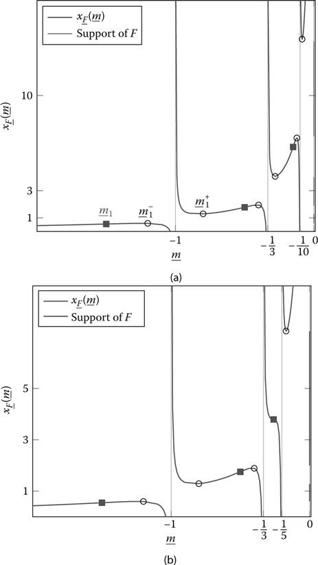
Figure 8.3:  x_F̲(m̲) for T_N diagonal composed of three evenly weighted masses in 1, 3, and 10 (a) and 1, 3, and 5 (b), c = 1/10 in both cases. Local extrema are marked in circles, inflexion points are marked in squares. The support of F can be read on the right vertical axes.

with ${\underset{\_}{m}}_1^{-}<{\underset{\_}{m}}_1^{+}\le {\underset{\_}{m}}_2^{-}<{\underset{\_}{m}}_2^{+}<\dots \le {\underset{\_}{m}}_{K_F}^{-}<{\underset{\_}{m}}_{K_F}^{+}$ the 2K_F (possibly counted with multiplicity) real roots of the equation in m̲,

${\displaystyle \sum _{r=1}^K{c}_r}\frac{t_r^2{\underset{\_}{m}}^2}{{\left(1+t_r{\underset{\_}{m}}^2\right)}^2}=1.$

Notice further from Figure 8.3 that, while x′_F̲(m̲) might not have roots on some intervals (−1/t_k−1, −1/t_k), it always has a unique inflexion point there. This is proved in [23] by observing that x″_F̲(m̲) = 0 is equivalent to

${\displaystyle \sum _{r=1}^K{c}_r}\frac{t_r^3{\underset{\_}{m}}^3}{{\left(1+t_r\underset{\_}{m}\right)}^3}-1=0,$

the left-hand side of which has always a positive derivative and shows asymptotes in the neighborhood of t_r; hence the existence of a unique inflexion point on every interval (−1/t_k−1, − 1/t_k), for 1 ≤ k ≤ K, with convention t₀ = 0+. When x_F̲ increases on an interval (−1/t_k−1, − 1/t_k), it must have its inflexion point in a point of positive derivative (from the concavity change induced by the asymptotes). Therefore, to verify that cluster k_F is disjoint from clusters (k − 1)_F and (k + 1)_F (when they exist), it suffices to verify that the (k − 1)^th and k^th roots m̲_k−1 and m̲_k of x″_F̲(m̲) are such that x′_F̲(m̲_k_₁) > 0 and x′_F̲(m̲_k) > 0. This is exactly what the following result states for the case of a sample covariance matrix whose population covariance matrix has few eigenvalues, each with a large multiplicity.

Theorem 8.3.7 ([23, 24]). Let B_N be defined as in Theorem 8.3.1, with T_N = diag (τ₁,…, τ_N) ∈ ℝ^N×N, diagonal containing K distinct eigenvalues 0 < t₁ < … < t_K, for some fixed K. Denote N_k the multiplicity of the k^th largest eigenvalue, counted with multiplicity (assuming ordering of the τ_i, we may then have τ₁ = … = ${\tau }_{N_1}=t_1,\dots ,{\tau }_{N-N_{K+1}}=\dots {\tau }_N=t_K$). Assume also that for all 1 ≤ r ≥ K, N_r/n → c_r > 0, and N/n → c, with 0 < c < ∞. Then the cluster k_F associated to the eigenvalue t_k in the l.s.d. F of B_N is distinct from the clusters (k − 1)_F and (k + 1)_F (when they exist), associated to t_k−1 and t_k+1 in F, respectively, if and only if

$\begin{array}{l}{\displaystyle \sum _{r=1}^K{c}_r}\frac{t_r^3{\underset{\_}{m}}_k^2}{{\left(1+t_r{\underset{\_}{m}}_k^2\right)}^2}<1,\\ {\displaystyle \sum _{r=1}^K{c}_r}\frac{t_r^3{\underset{\_}{m}}_{k+1}^2}{{\left(1+t_r{\underset{\_}{m}}_{k+1}^2\right)}^2}<1,\end{array}$

(8.13)

where m̲₁, …, m̲_K are such that m̲_K+1 = 0 and m̲₁ < m̲₂ < … < m̲_K are the K solutions of the equation in m̲,

${\displaystyle \sum _{r=1}^K{c}_r}\frac{t_r^3{\underset{\_}{m}}^3}{{\left(1+t_r\underset{\_}{m}\right)}^3}=1.$

For k = 1, this condition ensures 1_F = 2_F − 1; for k = K, this ensures K_F = (K − 1)_{F +1}; and for 1 < k < K, this ensures (k − 1)_F+1 = k_F = (k + 1)_{F− 1}.

This result is again fundamental in the sense that the separability of subsequent clusters in the support of the l.s.d. of B_N will play a fundamental role in the validity of statistical inference methods. In the subsequent section, we introduce the key ideas that allow statistical inference for sample covariance matrices.

8.4      Statistical Inference

Statistical inference allows for the estimation of deterministic parameters present in a stochastic model based on observations of random realizations of the model. In the context of sample covariance matrices, statistical inference methods consist in providing estimates of functionals of the eigenvalue distribution of the population covariance matrix T_N ∈ ℂ^N×N based on the observation ${\text{Y}}_N={\text{T}}_N^{\frac{1}{2}}{\mathbf{\text{X}}}_N$ with X_N ∈ ℂ^N×n a random matrix of independent and identically distributed entries. Different methods exist that allow for statistical inference that mostly rely on the study of the l.s.d. of the sample covariance matrix ${\mathbf{\text{B}}}_N=\frac{1}{n}{\text{Y}}_N{\text{Y}}_N^{†}$. One of these methods relates to free probability theory [25], and more specifically to free deconvolution approaches, see e.g., [26], [27]. The idea behind free deconvolution is based on the fact that the moments of the l.s.d. of some random matrix models can be written as a polynomial function of the moments of the l.s.d. of another (random) matrix in the model, under some proper conditions. Typically, the moments of the l.s.d. of T_N can be written as a polynomial of the moments of the (almost sure) l.s.d. of B_N, if X_N has Gaussian entries and the e.s.d. of T_N has uniformly bounded support. Therefore, to put it simply, one can obtain all moments of T_N based on a sufficiently large observation of B_N; this allows one to recover the l.s.d. of T_N (since Carleman condition is satisfied) and therefore any functional of the l.s.d. However natural, this method has some major drawbacks. From a practical point of view, a reliable estimation of moments of high order requires extremely large dimensional matrix observations. This is due to the fact that the estimate of the moment of order k of the l.s.d. is based on polynomial expressions of the estimates of moments of lower orders. A small error in the estimate in a low order moment therefore propagates as a large error for higher moments; it is therefore compelling to obtain accurate first order estimates, hence large dimensional observations.

We will not further investigate the moment-based approach above, which we discuss in more detail with a proper introduction to free probability theory in [28]. Instead, we introduce the methods based on the Stieltjes transform and those rely strongly on the results described in the previous section. We will introduce this method for the sample covariance matrix model discussed so far, because it will be instrumental to understanding the power estimator introduced in Section 8.5.2. Similar results have been provided for other models of interest to telecommunications, as for instance the so-called information-plus-noise model, studied in [29].

The central idea is based on a trivial application of the Cauchy complex integration formula [30]. Consider f some complex holomorphic function on U ⊂ ℂ, H a distribution function and denote G the functional

$G\left(f\right)={\displaystyle \int f\left(z\right)dH\left(z\right).}$

From the Cauchy integration formula, we have, for a negatively oriented closed path γ enclosing the support of H and with winding number one,

$\begin{array}{lll}\hfill G\left(f\right)& =\hfill & \frac{1}{2\pi i}{\displaystyle \int {\displaystyle {\oint }_{\text{γ}}\frac{f\left(\omega \right)}{z-\omega }d\omega dH\left(z\right)}}\hfill \\ \hfill & =\hfill & \frac{1}{2\pi i}{\displaystyle {\oint }_{\text{γ}}{\displaystyle \int \frac{f\left(\omega \right)}{z-\omega }dH\left(z\right)d\omega }}\hfill \\ \hfill & =\hfill & \frac{1}{2\pi i}{\displaystyle {\oint }_{\gamma }f\left(\omega \right)m_H\left(\omega \right)d\omega ,}\hfill \end{array}$

(8.14)

the integral inversion being valid since f (ω)/(z − ω) is bounded for ω ∈ γ. Note that the sign inversion due to the negative contour orientation is compensated by the sign reversal of (ω − z) in the denominator.

If dH is a sum of finite or countable masses and one is interested in evaluating f (λ_k), with λ_k the value of the k^th mass with weight l_k, then on a negatively oriented contour λ_k enclosing λ_k and excluding λ_j, j ≠ k,

$l_{k}f\left({\text{λ}}_k\right)=\frac{1}{2\pi i}{\displaystyle {\oint }_{\text{γ}k}f\left(\omega \right)m_H}\left(\omega \right)d\omega .$

(8.15)

This last expression is particularly convenient when one has access to H only through an expression of its Stieltjes transform.

Now, in terms of random matrices, for the sample covariance matrix ${\mathbf{\text{B}}}_N={\mathbf{\text{T}}}_N^{\frac{1}{2}}{\mathbf{\text{X}}}_N{\mathbf{\text{X}}}_N^{†}{\mathbf{\text{T}}}_N^{\frac{1}{2}}$, we already noticed that the l.s.d. F of B_N (or equivalently the l.s.d. F̲ of ${\underset{\_}{\mathbf{\text{B}}}}_N={\mathbf{\text{X}}}_N^{†}{\mathbf{\text{T}}}_N{\mathbf{\text{X}}}_N$) can be rewritten under the form (8.9), which can further be rewritten

$\frac{c}{m\underset{\_}{F}\left(z\right)}{m}_H\left(-\frac{1}{m\underset{\_}{F}\left(z\right)}\right)=-zm\underset{\_}{F}\left(z\right)+\left(c-1\right),$

(8.16)

where H is the l.s.d. of T_N. Note that it is allowed to evaluate m_H in −1/m_F̲(z) for z ∈ ℂ⁺ since −1/m_F̲(z) ∈ ℂ⁺.

As a consequence, if one only has access to $F^{B_N}$ (from the observation B_N), then the only link from the observation to H is obtained by (i) the fact that $F^{{\underset{\_}{\text{B}}}_N}\Rightarrow \underset{\_}{F}$ almost surely and (ii) the fact that F̲ and H are related through (8.16). Evaluating a functional f of the eigenvalue λ_k of T_N is then made possible by (8.15) . The relations (8.15) and (8.16) are the essential ingredients behind the derivation of a consistent estimator for f (λ_k).

We now concentrate specifically on the sample covariance matrix ${\underset{\_}{\mathbf{\text{B}}}}_N={\mathbf{\text{T}}}_N^{\frac{1}{2}}{\mathbf{\text{X}}}_N{\mathbf{\text{X}}}_N^{†}{\mathbf{\text{T}}}_N$ defined as in Theorem 8.3.1 with T_N composed of K distinct eigenvalues t₁,…, t_K of multiplicities N₁,…, N_K, respectively. We further denote c_k ≜ lim_n N_k/n and will discuss the question of estimating t_k itself. What follows summarizes the original ideas of Mestre in [22] and [24]. We have from (8.15) that, for any continuous f and for any negatively oriented contour C_k that encloses t_k and t_k only, f (t_k) can be written under the form

$\begin{array}{lll}\frac{N_k}{N}f\left(t_k\right)\hfill & =\hfill & \frac{1}{2\pi i}{\displaystyle {\oint }_{C_k}f\left(\omega \right)m_H\left(\omega \right)d\omega }\hfill \\ \hfill & =\hfill & \frac{1}{2\pi i}{\displaystyle {\oint }_{C_k}\frac{1}{N}{\displaystyle \sum _{r=1}^K{N}_r\frac{f\left(\omega \right)}{t_r-\omega }d\omega }}\hfill \\ \hfill & \hfill & \hfill \end{array}$

with H the limit $F^{T_N}\Rightarrow H$. This provides a link between f (t_k) for all continuous f and the Stieltjes transform m_H(z).

Letting f (x) = x and taking the limit N → ∞, N_k/N → c_k/c, with c ≜ c₁ + … + c_K the limit of N/n, we have

$\frac{c_k}{c}{t}_k=\frac{1}{2\pi i}{\displaystyle {\oint }_{C_k}\omega m_H\left(\omega \right)d\omega }.$

(8.17)

We now want to express m_H as a function of m_F, the Stieltjes transform of the l.s.d. F of B_N. For this, we have the two relations (8.10), i.e.,

$m\underset{\_}{F}\left(z\right)=c{m}_F\left(z\right)+\left(c-1\right)\frac{1}{z}$

and (8.16) with F^T = H, i.e.,

$\frac{c}{m_{\underset{\_}{F}}\left(z\right)}{m}_H\left(-\frac{1}{m_{\underset{\_}{F}}\left(z\right)}\right)=-z{m}_{\underset{\_}{F}}\left(z\right)+\left(c-1\right).$

Together, those two equations give the simpler expression

$m_H\left(-\frac{1}{m_{\underset{\_}{F}}\left(z\right)}\right)=-z{m}_{\underset{\_}{F}}\left(z\right)m_F\left(z\right).$

Applying the variable change ω = −1/m_F̲(z) in (8.17), we obtain

$\begin{array}{lll}\frac{c_k}{c}{t}_k\hfill & =\hfill & \frac{1}{2\pi i}{\displaystyle {\oint }_{C_{\underset{\_}{F},k}}z\frac{m_{\underset{\_}{F}}\left(z\right){m^{\prime }}_{\underset{\_}{F}}\left(z\right)}{c}}+\frac{1-c}{c}\frac{m_{\underset{\_}{F}}{\left(z\right)}^{\prime }}{m_{\underset{\_}{F}}^2\left(z\right)}dz\hfill \\ \hfill & =\hfill & \frac{1}{c}\frac{1}{2\pi i}{\displaystyle {\oint }_{C_{\underset{\_}{F},k}}z\frac{{m^{\prime }}_{\underset{\_}{F}}\left(z\right)}{m\underset{\_}{F}\left(z\right)}dz,}\hfill \end{array}$

(8.18)

where C_F̲,k is the preimage of C_F̲ by −1/m_F̲. The second equality (8.18) comes from the fact that the second term in the previous relation is the derivative of (c − 1) / (cm_F̲(z)), which therefore integrates to 0 on a closed path, from classical real or complex integration rules [30]. Obviously, since z ∈ ℂ⁺ is equivalent to − 1/m_F̲(z) ∈ ℂ⁺ (the same being true if ℂ⁺ is replaced by ℂ⁻), C_F̲ ,_k is clearly continuous and of non-zero imaginary part whenever $\mathfrak{I}$(z) = 0. Now, one must be careful about the exact choice of C_F̲ ,_k.

We make the important assumption that the index k satisfies the separability conditions of Theorem 8.3.7. That is, the cluster k_F associated to k in F is distinct from (k − 1)_F and (k + 1)_F (whenever they exist). Let us then pick $x_F^{\left(l\right)}$ and $x_F^{\left(r\right)}$ two real values such that

$x_{\left(k-1\right)F}^{+}<x_F^{\left(l\right)}<x_{k_F}^{-}<x_{k_F}^{+}<x_F^{\left(r\right)}<x_{\left(k+1\right)F}^{-}$

with $\left\{x_1^{-},x_1^{+},\dots ,x_{K_F}^{-},x_{K_F}^{+}\right\}$ the support boundary of F, as defined in Theorem 8.3.6. Now remember Theorem 8.3.5 and Figure 8.3; for $x_F^{\left(l\right)}$ as defined previously, m_F̲ (z) has a limit m^(l) ∈ ℝ as $z\to x_F^{\left(l\right)},z\in {ℂ}^{+}$, and a limit m^(r) ∈ ℝ as $z\to x_F^{\left(r\right)},z\in {ℂ}^{+}$, those two limits verifying

$t_{k-1}<x^{\left(l\right)}<t_k<x^{\left(r\right)}<t_{k+1},$

(8.19)

with x^(l) = − 1/m^(l) and x^(r) = − 1/m^(r).

This is the most important outcome of the integration process. Let us define C_F̲,k to be any continuous contour surrounding cluster k_F such that C_F̲,k crosses the real axis in only two points, namely $x_F^{\left(l\right)}$ and $x_F^{\left(r\right)}$. Since −1/m_F̲(ℂ⁺) ⊂ ℂ⁺ and −1/m_F̲(ℂ⁺) ⊂ ℂ⁺, C_k does not cross the real axis whenever $\mathfrak{I}$(z) ≠ 0 and is obviously continuously differentiable there; now C_k crosses the real axis in x^(l) and x^(r), and is in fact continuous there. Because of (8.19), we then have that C_k is (at least) continuous and piecewise continuously differentiable and encloses only t_k. This is what is required to ensure the validity of (8.18).

The difficult part of the proof is completed. The rest will unfold more naturally. We start by considering the following expression,

$\begin{array}{lll}{\widehat{t}}_k\hfill & \triangleq \frac{1}{2\pi i}\frac{n}{N_k}{\displaystyle {\oint }_{C_{\underset{\_}{F},k}}z\frac{{m^{\prime }}_{F^{\underset{\_}{\mathbf{\text{B}}}}N}\left(z\right)}{m_{F^{\underset{\_}{\mathbf{\text{B}}}}N}\left(z\right)}dz}\hfill & \hfill \\ \hfill & =\frac{1}{2\pi i}\frac{n}{N_k}{\displaystyle {\oint }_{C_{\underset{\_}{F},k}}z\frac{\frac{1}{n}{\displaystyle {\sum }_{i=1}^n\frac{1}{{\left({\text{λ}}_i-z\right)}^2}}}{\frac{1}{n}{\displaystyle {\sum }_{i=1}^n\frac{1}{{\text{λ}}_i-z}}}dz,}\hfill & \hfill \end{array}$

(8.20)

where we remind that ${\underset{\_}{\mathbf{\text{B}}}}_N\underset{\_}{\underset{\_}{\Delta }}{\mathbf{\text{X}}}_N^{†}{\mathbf{\text{T}}}_N{\mathbf{\text{X}}}_N$ and where, if n ≥ N, we defined λ_N+1 = … =λ_n = 0.

The value t̂_k can be viewed as the empirical counterpart of t_k. Now, we know from Theorem 8.2.9 that $m_{F^{\mathbf{\text{B}}}N}\left(z\right)\underrightarrow{\text{a}.\text{s}.}{m}_F\left(z\right)$ and $m_{F^{\underset{\_}{\mathbf{\text{B}}}}N}\left(z\right)\to m_{\underset{\_}{F}}\left(z\right)$. It is not difficult to verify, from the fact that m_F̲ is holomorphic, that the same convergence holds for the successive derivatives.

At this point, we need the two fundamental results that are Theorem 8.3.1 and Theorem 8.3.4. We know that, for all matrices B_N in a set of probability one, all the eigenvalues of B_N are contained in the support of F for all large N, and that the eigenvalues of B_N contained in cluster k_F are exactly {λ_i, i ∈ $\mathcal{N}$_k} for these large $\mathcal{N}$, with ${\mathcal{N}}_k\left\{{\displaystyle {\sum }_{j=1}^{k-1}{N}_j+1,\dots ,}{\displaystyle {\sum }_{j=1}^k{N}_j}\right\}$. Take such a B_N. For all large $N,m_{{\mathbf{\text{B}}}_N}\left(z\right)$ is uniformly bounded over N and z ∈ C_F̲,k, since C_F̲,k is away from the support of F. The integrand on the right-hand side of (8.20) is then uniformly bounded for all large N and for all z ∈ C_F̲,k. By the dominated convergence theorem, Theorem 16.4 in [16], we then have that ${\widehat{t}}_k-t_k\underrightarrow{\text{a}.\text{s}.}0$.

It then remains to evaluate t̂_k explicitly. This is performed by residue calculus [30], i.e., by determining the poles in the expanded expression of t̂_k (when developing $m_{F^{\mathbf{\text{B}}}N}\left(z\right)$ in its full expression). Those poles are found to be λ₁,…, λ_N (indeed, the integrand of (8.20) behaves like O(1/(λ_i − z)) for z ≃ λ_i) and μ₁,…, μ_N, the N real roots of the equation in $\mu ,m_{F^{\mathbf{\text{B}}}N}\left(\mu \right)=0$ (indeed, the denominator of the integrand cancels for z = μ_i while the numerator is non-zero). Since C_F̲,k encloses only those values λ_i such that i ∈ $\mathcal{V}$_k, the other poles are discarded. Noticing now that $m_{F^{\mathbf{\text{B}}}N}\left(\mu \right)=\pm \infty$ as μ → A_i, we deduce that μ₁ < μ₁ < μ₂ < … < μ_N < λ_N, and therefore we have that μ_i,j ∈ $\mathcal{N}$_k are all in C_F̲,k but maybe for μ_j, j = min N_k. It can in fact be shown that μ_j is also in C_F̲,k. To notice this last remaining fact, observe simply that

$\frac{1}{2\pi i}{\displaystyle {\oint }_{C_k}\frac{1}{\omega }d\omega =0.}$

since 0 is not contained in the contour C_k. Applying the variable change ω = −1/m_F̲ (z) as previously, this gives

${\displaystyle {\oint }_{C_{\underset{\_}{F},}{}_k}\frac{{m^{\prime }}_{\underset{\_}{F}}\left(z\right)}{m_{\underset{\_}{F}}^2\left(z\right)}dz=0.}$

(8.21)

From the same reasoning as above, with the dominated convergence theorem argument, we have that for sufficiently large N and almost surely,

$\left|{\displaystyle {\oint }_{C_{\underset{\_}{F},}{}_k}\frac{{m^{\prime }}_{F^{\underset{\_}{\mathbf{\text{B}}}}N}\left(z\right)}{m_{F^{\underset{\_}{\mathbf{\text{B}}}}N}^2\left(z\right)}dz}\right|<\frac{1}{2}.$

(8.22)

At this point, we need to proceed to residue calculus in order to compute the integral on the left-hand side of (8.22). We will in fact prove that the value of this integral is an integer, hence necessarily equal to zero from the inequality (8.22) . Notice indeed that the poles of (8.21) are the λ_i and the μ_i that lie inside the integration contour C_F̲,k, all of order one with residues equal to −1 and 1, respectively. Therefore, (8.21) equals the number of such λ_i minus the number of such μ_i (remember that the integration contour is negatively oriented, so we need to reverse the signs). We, however, already know that this difference, for large N, equals either 0 or 1, since only the position of the leftmost μ_i is unknown yet. But since the integral is asymptotically less than 1/2, this implies that it is identically zero, and therefore the leftmost μ_i (indexed by min $\mathcal{N}$_k) also lies inside the integration contour.

From this point on, we can evaluate (8.20), which is clearly determined since we know exactly which eigenvalues of B_N are contained (with probability one for all large N) within the integration contour. This calls again for residue calculus, the steps of which are detailed below. Denoting

$f\left(z\right)=z\frac{{m^{\prime }}_{F^{\underset{\_}{\mathbf{\text{B}}}}N}\left(z\right)}{m_{F^{\underset{\_}{\mathbf{\text{B}}}}N}^{}\left(z\right)},$

we find that λ_i (inside C_F̲,k) is a pole of order 1 with residue

$\underset{z\to {\text{λ}}_i}{\lim }\left(z-{\text{λ}}_i\right)f\left(z\right)=-{\text{λ}}_i,$

which is straightforwardly obtained from the fact that $f\left(z\right)\sim \frac{1}{{\text{λ}}_i-z}$ as z ~ λ_i. Also μ_i (inside C_F̲,k) is a pole of order 1 with residue

$\underset{z\to {\mu }_i}{\lim }\left(z-{\mu }_i\right)f\left(z\right)=-{\mu }_i.$

Since the integration contour is chosen to be negatively oriented, it must be kept in mind that the signs of the residues need be inverted in the final relation.

Noticing finally that μ₁,…, μ_N are also the eigenvalues of diag $\left(\text{λ}\right)-\frac{1}{n}\sqrt{\text{λ}}{\sqrt{\text{λ}}}^T$, with λ ≜ (λ₁,…, A_N)^T, from a lemma provided in [23, Lemma 1] and [31], we finally have the following statistical inference result for sample covariance matrices.

Theorem 8.4.1 ([24]). Let ${\mathbf{\text{B}}}_N{\mathbf{\text{=T}}}_N^{\frac{1}{2}}{\mathbf{\text{X}}}_N{\mathbf{\text{X}}}_N^{†}{\mathbf{\text{T}}}_N^{\frac{1}{2}}\in {ℂ}^{N\times N}$ be defined as in Theorem 8.3.7, i.e., T_N has K distinct eigenvalues t₁ < … < t_K with multiplicities N₁, …, N_K, respectively, for all r, N_r/n → c_r , 0 < c_r < ∞, and the separability conditions (8.13) are satisfied. Further denote λ₁ < … ≤ λ_N the eigenvalues of B_N and λ = (λ₁, …, λ_N)^T. Let k ∈ {1, …, K}, and define

${\widehat{t}}_k=\frac{n}{N_k}{\displaystyle \sum _{m\in {\mathcal{N}}_k}\left({\text{λ}}_m-{\mu }_m\right)}$

(8.23)

with ${\mathcal{N}}_k\left\{{\displaystyle {\sum }_{j=1}^{k-1}{N}_j+1,\dots ,}{\displaystyle {\sum }_{j=1}^k{N}_j}\right\}$ and μ₁ ≤ … ≤ are the ordered eigenvalues of the matrix diag $\left(\text{λ}\right)-\frac{1}{n}\sqrt{\text{λ}}{\sqrt{\text{λ}}}^T$.

Then, if condition (8.13) is fulfilled, we have

${\widehat{t}}_k-t_k\to 0$

almost surely as N,n → ∞, N/n → c, 0 < c < ∞.

Similarly, for the quadratic form, the following holds.

Figure 8.4:  Estimation of t₁,t₂,t₃ in the model ${\mathbf{\text{B}}}_N{\text{=T}}_N^{\frac{1}{2}}{\mathbf{\text{X}}}_N{\mathbf{\text{X}}}_N^{†}{\mathbf{\text{T}}}_N^{\frac{1}{2}}$ based on the first three empirical moments of B_N and Newton-Girard inversion, see [32], for N₁/N = N₂/N = N₃/N = 1/3, N/n = 1/10, for 100,000 simulation runs; (a) N = 30, n = 90; (b) N = 90, n = 270. Comparison is made against the Stieltjes transform estimator of Theorem 8.4.1.

Theorem 8.4.2 ([24]). Let B_N be defined as in Theorem 8.4.1, and denote ${\mathbf{\text{B}}}_N={\displaystyle {\sum }_{k=1}^N{\text{λ}}_k{\text{b}}_k{\text{b}}_k^{†},}{\text{b}}_k^{†}{\text{b}}_i={\delta }_k^i$, the spectral decomposition of B_N. Similarly, denote ${\mathbf{\text{T}}}_N={\displaystyle {\sum }_{k=1}^K{t}_k{\mathbf{\text{U}}}_k{\mathbf{\text{U}}}_k^{†},}{\mathbf{\text{U}}}_k^{†}{\mathbf{\text{U}}}_k={\text{I}}_{n_k}$, with ${\mathbf{\text{U}}}_k\in {ℂ}^{N\times N_k}$ the eigenspace associated to t_k. For given vectors x, γ ∈ ℂ^N, denote

$u\left(k;x,y\right)\triangleq x^{†}{U}_k{U}_k^{†}y.$

Then we have

$\widehat{u}\left(k;x,y\right)-u\left(k;x,y\right)\stackrel{\text{a}.\text{s}.}{\to }0$

as N,n → ∞ with ratio c_N = N/n → c, where

$\widehat{u}\left(k;x,y\right)\triangleq {\displaystyle \sum _{i=1}^N{\theta }_k\left(i\right)x^{†}{b}_k}{b}_k^{†}y$

and θ_k (i) is defined by

${\theta }_i\left(k\right)=\{\begin{array}{ll}-{\varphi }_k\left(i\right)\hfill & ,i\notin {\mathcal{N}}_k\hfill \\ 1+{\psi }_k\left(i\right)\hfill & ,i\in {\mathcal{N}}_k,\hfill \end{array}$

with

$\begin{array}{l}{\varphi }_k\left(i\right)={\displaystyle \sum _{r\in {\mathcal{N}}_k}\left(\frac{{\text{λ}}_r}{{\text{λ}}_i-{\text{λ}}_r}-\frac{{\mu }_r}{{\text{λ}}_i-{\mu }_r}\right)},\\ {\psi }_k\left(i\right)={\displaystyle \sum _{r\notin {\mathcal{N}}_k}\left(\frac{{\text{λ}}_r}{{\text{λ}}_i-{\text{λ}}_r}-\frac{{\mu }_r}{{\text{λ}}_i-{\mu }_r}\right)}\end{array}$

and N_k , μ₁,…, μ_N defined as in Theorem 8.4.1.

The estimator proposed in Theorem 8.4.1 is extremely accurate and is in fact much more flexible and precise than free deconvolution approaches. A visual comparison is proposed in Figure 8.4 for the same scenario as in Figure 8.3, where the free deconvolution (also called moment-based) method is based on the inference techniques proposed in e.g., [26, 32]. Nonetheless, it must be stressed that the cluster separability condition, necessary to the validity of the Stieltjes transform approach, is mandatory and sometimes a rather strong assumption. Typically, the number of observations must be rather large compared to the number of sensors in order to be able to resolve close values of t_k.

8.5      Applications

In this section, we apply the random matrix methods developed above to the problems of multidimensional binary hypothesis testing and parameter estimation. More details on these applications as well as a more exhaustive list of applications, notably in the field of wireless communications, are provided in [28].

8.5.1      Binary Hypothesis Testing

We first consider the problem of detecting the presence of a signal source impaired by white Gaussian noise. The question is therefore to decide whether only noise is being sensed or if some data plus noise are sensed.

Precisely, we consider a signal source or transmitter of dimension K and a sink or receiver composed of N sensors. The linear filter between the transmitter and the receiver is modelled by the matrix H ∈ ℂ^N×K, with (i, j)^th entries h_ij. If at time l the transmitter emits data, those are denoted by the K-dimensional vector ${\text{x}}^{\left(l\right)}=\left(x_1^{\left(l\right)},\dots ,x_K^{\left(l\right)}\right)\in {ℂ}^K$. The additive white Gaussian noise at the receiver is modelled, at time l, by the vector $\sigma {\text{w}}^{\left(l\right)}=\sigma {\left({\omega }_1^{\left(l\right)},\dots {\omega }_N^{\left(l\right)}\right)}^T\in {ℂ}^N$, where σ² denotes the variance of the noise vector entries. Without generality restriction, we consider in the following zero mean and unit variance of the entries of both w⁽¹⁾ and x⁽¹⁾, i.e., $E\left\{{\left|w_i^{\left(l\right)}\right|}^2\right\}=1,E\left\{{\left|w_i^{\left(l\right)}\right|}^2\right\}=1$ for all i. We then denote ${\text{y}}^{\left(l\right)}={\left(y_1^{\left(l\right)},\dots ,y_N^{\left(l\right)}\right)}^T$ the N-dimensional data received at time l. Assuming the filter is static during at least M sampling periods, we finally denote Y = [y⁽¹⁾,…, y^(M)] ∈ ℂ^N×N the matrix of the concatenated received vectors.

Depending on whether the transmitter emits data, we consider the following hypotheses

•  $\mathcal{H}$₀. Only background noise is received.

•  $\mathcal{H}$₁. Data plus background noise are received.

Therefore, under condition $\mathcal{H}$₀, we have the model

$Y=\sigma W$

with W = [w⁽¹⁾,…, w^(M)] ∈ ℂ^N×N and under condition H₁

$Y=\left(H\sigma I_N\right)\left(\begin{array}{l}X\hfill \\ W\hfill \end{array}\right)$

(8.24)

with X = [x⁽¹⁾,…, x^(M)] ∈ ℂ^N×N.

Under this hypothesis, we further denote ∑ the covariance matrix of y⁽¹⁾,

$\sum =E\left\{{\text{y}}^{\left(1\right)}{\left({\text{y}}^{\left(1\right)}\right)}^{†}\right\}=H{H}^{†}+{\sigma }^2{I}_N=UG{U}^{†}$

where G = diag (ν₁ + σ²,…, ν_N + σ²) ∈ ℝ^N×N, with {ν₁,…, v_N} the eigenvalues of HH^† and U ∈ ℂ^N×N a certain unitary matrix.

The receiver is entitled to decide whether data were transmitted or not. It is a common assumption to be in the scenario where σ² is known in advance, although it is uncommon to know the transfer matrix H. This is true in particular of the wireless signal sensing scenario where H is the wireless fading channel matrix between two antenna arrays. We consider specifically the scenario where the probability distribution of H is unitarily invariant, which is in particular consistent in wireless communications with channel models that do not a priori exhibit specific directions of energy propagation. This is in particular relevant when the filter H presents rotational invariance properties. For simplicity we take H and x^(l) to be i.i.d. Gaussian with zero mean and E {∣h_ij∣²} = 1/K, although our study could go well beyond the Gaussian case.

For simplicity, we consider in the following K = 1, although a generalized result exists for K ≥ 1 [2]. The Neyman-Pearson criterion for the receiver to establish whether data were transmitted is based on the ratio

$C\left(Y\right)=\frac{\text{Pr}{}_{{\mathscr{H}}_{\text{1}}|Y}\left(Y\right)}{\text{Pr}{}_{{\mathscr{H}}_{\text{0}}|Y}\left(Y\right)},$

(8.25)

where ${\text{Pr}}_{{\mathscr{H}}_i|Y}\left(\mathbf{\text{Y}}\right)$ is the probability of the event H_i conditioned on the observation Y. For a given receive space-time matrix Y, if C(Y) > 1, then the odds are that an informative signal was transmitted, while if C(Y) < 1, it is more likely that only background noise was captured. To ensure a low probability of false alarm (or false positive), i.e., the probability to declare a pure noise sample to carry an informative signal, a certain threshold ξ is generally set such that, when C(Y) > ξ, the receiver declares data were transmitted, while when C(Y) < ξ the receiver declares that no data were sent. The question of what ratio ξ should be set to ensure a given maximally acceptable false alarm rate will not be treated here. We will however provide an explicit expression of (8.25) for the aforementioned model, and shall compare its performance to that achieved by the classical energy detector. The results provided in this section are taken from [2].

Applying Bayes’ rule, (8.25) becomes

$C\left(Y\right)=\frac{\text{Pr}{}_{{\mathscr{H}}_{\text{0}}}\cdot \text{Pr}{}_{{\mathscr{H}}_{\text{1}}|Y}\left(Y\right)}{\text{Pr}{}_{{\mathscr{H}}_{\text{1}}}\cdot \text{Pr}{}_{{\mathscr{H}}_{\text{0}}|Y}\left(Y\right)},$

with ${\text{Pr}}_{{\mathcal{H}}_i}$ the a priori probability for hypothesis $\mathcal{H}$_i to hold. We suppose that no side information allows the receiver to consider that $\mathcal{H}$₁ is more or less probable than $\mathcal{H}$₀, and therefore set ${\text{Pr}}_{{\mathscr{H}}_0}={\text{Pr}}_{{\mathscr{H}}_1}=\frac{1}{2}$, so that

$C\left(Y\right)=\frac{\text{Pr}{}_{{\mathscr{H}}_{\text{1}}|Y}\left(Y\right)}{\text{Pr}{}_{{\mathscr{H}}_{\text{0}}|Y}\left(Y\right)},$

(8.26)

reduces to a maximum likelihood ratio.

Likelihood under $\mathcal{H}$₀. In this first scenario, the noise entries $w_i^{\left(l\right)}$ are Gaussian and independent. The probability density of Y, which can be seen as a random vector with NM entries, is then an NM multivariate uncorrelated complex Gaussian with covariance matrix σ² I_NM,

$\begin{array}{c}\mathrm{Pr}\\ \mathbf{\text{Y}}|{\mathscr{H}}_0\end{array}\left(Y\right)=\frac{1}{{\left(\pi {\sigma }^2\right)}^{NM}}{e}^{-\frac{1}{{\sigma }^2}\text{tr}\left(Y{Y}^{†}\right)}.$

(8.27)

Denoting λ = (λ₁,…, λ_N)^T the eigenvalues of YY^†, (8.27) only depends on ${\displaystyle {\sum }_{i=1}^N{\text{λ}}_i}$, as follows

$\begin{array}{c}\mathrm{Pr}\\ \mathbf{\text{Y}}|{\mathscr{H}}_0\end{array}\left(Y\right)=\frac{1}{{\left(\pi {\sigma }^2\right)}^{NM}}{e}^{-\frac{1}{{\sigma }^2}{\displaystyle {\sum }_{i=1}^N{\text{λ}}_i}}.$

Likelihood under $\mathcal{H}$₁. Under the data plus noise hypothesis $\mathcal{H}$₁, the problem is more involved. The entries of the channel matrix H are modeled as jointly uncorrelated Gaussian, with E {∣h_ij∣²} = 1/K. Therefore, since here K =1, H ∈ ℂ^N×1 and ∑ = HH^† + σ²I_N has N − 1 eigenvalues g₂ = ⋯ = g_N equal to σ² and another distinct eigenvalue $g_1=v_1+{\sigma }^2\left({\displaystyle {\sum }_{i=1}^N{\left|h_{i1}\right|}^2}\right)+{\sigma }^2$. The density of g₁ − σ² is a complex chi-square distribution of N degrees of freedom (denoted ${\mathcal{X}}_N^2$), which up to a scaling factor 2 is equivalent to a real ${\mathcal{X}}_{2N}^2$ distribution. Hence, the eigenvalue distribution of ∑, defined on ℝ^+N = [0, ∞)^N, reads

$\begin{array}{c}\mathrm{Pr}\\ \text{G}\end{array}\left(G\right)=\frac{1}{N}\left({\left(g_1-{\sigma }^2\right)}_{+}^{N-1}\right)\frac{e^{-\left(g_1-{\sigma }^2\right)}}{\left(N-1\right)!}{\displaystyle \prod _{i=2}^N\left(g_i-{\sigma }^2\right).}$

From the model $\mathcal{H}$₁, Y is distributed as correlated Gaussian, as follows

$\begin{array}{c}\mathrm{Pr}\\ \mathbf{\text{Y}}|\sum ,I_1\end{array}\left(Y,\sum \right)=\frac{1}{{\pi }^{MN}\text{det}{\left(G\right)}^M}{e}^{-\text{tr}\left(Y{Y}^{†}U{G}^{-1}{U}^{†}\right)},$

where I_k denotes the prior information at the receiver “$\mathcal{H}$₁ and K = k.”

Since H is unknown, we need to integrate out all possible linear filters for the transmission model under $\mathcal{H}$₁ over the probability space of N × K matrices with Gaussian i.i.d. distribution. From the invariance of Gaussian i.i.d. random matrices by left and right products with unitary matrices, this is equivalent to integrating out all possible covariance matrices ∑ over the space of such nonnegative definite Hermitian matrices, as follows

$\begin{array}{c}\mathrm{Pr}\\ \mathbf{\text{Y}}|{\mathscr{H}}_1\end{array}\left(Y\right)={\displaystyle \underset{\sum }{\int }\begin{array}{c}\mathrm{Pr}\\ \mathbf{\text{Y}}|\sum ,{\mathscr{H}}_1\end{array}}\left(Y,\sum \right)\begin{array}{c}\mathrm{Pr}\\ \sum \end{array}(\sum )d\sum .$

Eventually, after complete integration calculus given in the proof below, the Neyman-Pearson decision ratio (8.25) for the single-input multiple-output channel takes an explicit expression, given by the following theorem.

Theorem 8.5.1. The Neyman-Pearson test ratio C_Y(Y) for the presence of data reads

$C_Y\left(Y\right)=\frac{1}{N}{\displaystyle \sum _{l=1}^N\frac{{\sigma }^{2\left(N+M-1\right)}{e}^{{\sigma }^2+\frac{{\text{λ}}_l}{{\sigma }^2}}}{{\displaystyle \prod _{\begin{array}{l}i=1\\ i\ne l\end{array}}^N\left({\text{λ}}_l-{\text{λ}}_i\right)}}}{J}_{N-M-1}\left({\sigma }^2,{\text{λ}}_l\right)$

(8.28)

with λ₁, …, λ_N the eigenvalues of YY^† and where

$J_k\left(x,y\right)\triangleq {\displaystyle {\int }_x^{+\infty }{t}^k{e}^{-t-\frac{y}{t}}}dt.$

The proof of Theorem 8.5.1 is provided below. Among the interesting features of (8.28), note that the Neyman-Pearson test does only depend on the eigenvalues of YY^†. This suggests that the eigenvectors of YY^† do not provide any information regarding the presence of data. The essential reason is that, both under H₀ and $\mathcal{H}$₁, the eigenvectors of Y are isotropically distributed on the unit N-dimensional complex sphere due to the Gaussian assumptions made here. As such, a given realization of the eigenvectors of Y does indeed not carry any relevant information to the hypothesis test. The Gaussian assumption for H brought by the maximum entropy principle is in fact essential here. Note however that (8.28) is not reduced to a function of the sum ∑_i λ_i of the eigenvalues, as suggests the classical energy detector.

On the practical side, note that the integral J_k (x,y) does not take a closedform expression, but for x = 0, [33, see e.g., pp. 561]. This is rather inconvenient for practical purposes, since J_k (x, y) must either be evaluated every time, or be tabulated. It is also difficult to get any insight on the performance of such a detector for different values of σ², N and K. We provide hereafter a sketch of proof of Theorem 8.5.1, in which classical multidimensional integration techniques are introduced. In particular, the tools introduced in Section 8.2 will be shown to be key ingredients of the derivation.

Proof. We start by noticing that H is Gaussian and therefore that the joint density of its entries is invariant by left and right unitary products. As a consequence, the distribution of the matrix ∑ = HH^† + σ²I is unitarily invariant. This allows us to write

$\begin{array}{lll}\begin{array}{c}\text{Pr}\\ \mathbf{\text{Y}}|I_1\end{array}\left(Y\right)\hfill & =\hfill & \begin{array}{c}\text{Pr}\\ \mathbf{\text{Y}}|\text{Σ},{\mathscr{H}}_1\end{array}\left(Y,\sum \right)\begin{array}{c}\mathrm{Pr}\\ \sum \end{array}(\sum )d\sum \hfill \\ \hfill & =\hfill & {\displaystyle \underset{\mathcal{U}\left(N\right)\times {\left({ℝ}^{+}\right)}^N}{\int }\begin{array}{c}\text{Pr}\\ \mathbf{\text{Y}}|\text{Σ},{\mathscr{H}}_1\end{array}\left(Y,\sum \right)\begin{array}{c}\mathrm{Pr}\\ G\end{array}\left(G\right)dUdG}\hfill \\ \hfill & =\hfill & {\displaystyle \underset{\mathcal{U}\left(N\right)\times {ℝ}^{+}}{\int }\begin{array}{c}\text{Pr}\\ \mathbf{\text{Y}}|\text{Σ},{\mathscr{H}}_1\end{array}\left(Y,\sum \right)\begin{array}{c}\mathrm{Pr}\\ g_1\end{array}\left(g_1\right)dUd\left(g_1\right)}\hfill \end{array}$

with U(N) the space of N × N unitary matrices and ∑ = UGU^†.

The latter can further be equated to

$\begin{array}{c}\text{Pr}\\ \mathbf{\text{Y}}|I_1\end{array}\left(Y\right)={\displaystyle \underset{\mathcal{U}\left(N\right)\times {ℝ}^{+}}{\int }\frac{e^{-\text{tr}\left(Y{Y}^{†}U{G}^{-1}{U}^{†}\right)}}{{\pi }^{NM}\text{det}{\left(G\right)}^M}\left({\left(g_1-{\sigma }^2\right)}_{+}^{N-1}\right)\frac{e^{-\left(g_1-{\sigma }^2\right)}}{N!}dUd\left(g_1\right)}$

with (x)₊ ≜ max(x, 0) here.

To go further, we use the Harish–Chandra identity provided in Theorem 8.2.3. Denoting Δ(Z) the Vandermonde determinant of matrix Z ∈ ℂ^N×N with eigenvalues z₁ ≤ … ≤ z_N

$\text{Δ}\left(Z\right)\triangleq {\displaystyle \prod _{i>j}\left(z_i-z_j\right),}$

(8.29)

the likelihood ${\text{Pr}}_{\text{Y|}{I}_1}\left(\mathbf{\text{Y}}\right)$ reads

$\begin{array}{l}\begin{array}{c}\mathrm{Pr}\\ Y|I_1\end{array}(Y)=\left(\underset{g_2,\dots ,g_N\to {\sigma }^2}{\lim }\frac{e^{{\sigma }^2}{\left(-1\right)}^{\frac{N\left(N-1\right)}{2}}{\displaystyle \prod _{j=1}^{N-1}j!}}{{\pi }^{MN}{\sigma }^{2M\left(N-1\right)}N!}\right){\displaystyle \underset{{\sigma }^2}{\overset{+\infty }{\int }}\frac{1}{g_1^M}{\left(g_1-{\sigma }^2\right)}^{N-1}}\\ e^{-g_1}\frac{\text{det}\left(e^{-\frac{{\text{λ}}_i}{g_j}}\right)}{\text{Δ}\left(Y{Y}^{†}\right)\text{Δ}\left(G^{-1}\right)}d\left(g_1\right)\end{array}$

(8.30)

in which we remind that λ₁,…, λ_N are the eigenvalues of YY^†. Note the trick of replacing the known values of g₂,…, g_N by limits of scalars converging to these known values, which allows us to use correctly the Harish–Chandra formula. The remainder of the proof consists of deriving the explicit limits, which in particular relies on the following result [34, Lemma 6].

Theorem 8.5.2. Let f₁,…,f_N be a family of infinitely differentiable functions and let x₁,…, x_N ∈ ℝ. Denote

$R\left(x_1,\dots ,x_N\right)\triangleq \frac{\text{det}\left({\left\{f_i\left(x_j\right)\right\}}_{i,j}\right)}{{\displaystyle \prod _{i>j}\left(x_i-x_j\right)}}.$

Then, for p ≤ N and for x₀ ∈ ℝ,

$\underset{x_1,\dots ,x_p\to x_0}{\lim }R\left(x_1,\dots ,x_N\right)=\frac{\text{det}\left(f_i\left(x_0\right),{f^{\prime }}_i\left(x_0\right),\dots ,f_i^{\left(p-1\right)}\left(x_0\right),f_i\left(x_{p+1}\right),\dots ,f_i\left(x_N\right)\right)}{{\displaystyle \prod _{p<j<i}\left(x_i-x_j\right)}{\displaystyle \prod _{i=p+1}^N{\left(x_i-x_0\right)}^p}{\displaystyle \prod _{j=1}^{p-1}j!}}.$