Chapter 10  Fundamentals of Estimation Theory

Yik-Chung Wu^‡

^‡ University of Hong Kong

Parameter estimation is prevalent in communications and signal processing applications, e.g., in channel estimation, synchronization, parametric spectral estimation, direction-of-arrival estimation, etc. Estimation theory is extensively used in modern research in various fields related to signal processing. This chapter presents an overview of basic parameter estimation techniques and discusses the relationships among them. Applications in problems involving recent research are provided as examples.

10.1    Introduction

In an estimation problem, we have some observations which depend on the parameters we want to estimate. For example, the observations can be written as

$\text{x}=\text{f}\left(\theta \right)+\text{w,}$

(10.1)

where x stands for the observations, θ is the parameter we want to estimate, f is a known function, and w denotes the random noise corrupting the observations. All the above quantities can be in vector form. In this chapter, it is assumed that the dimension of x is N × 1 while that of θ is p × 1 with N > p. In general, x can depend on θ in a linear or nonlinear way. It is even possible that some of the elements of θ are related to x in a linear way, while others are related to x in a nonlinear way. The task of parameter estimation is to construct a function (called estimator) such that $\widehat{\theta }:=g\left(x\right)$ is a good estimate of θ. The first question we encounter is how to define a “good” estimate. One natural criterion is that the average squared difference between ${\widehat{\theta }}_i$ and θ_i should be the smallest, where θ_i is the i^th element of θ. Such squared difference is referred to as the MSE:

$\text{MSE}\left({\widehat{\theta }}_i\right)=E\left\{{\left({\widehat{\theta }}_i-{\theta }_i\right)}^2\right\},$

where expectation is taken with respect to the random noise w. If we rewrite the above expression as

$\begin{array}{l}\text{MSE}\left({\widehat{\theta }}_i\right)=E\left\{{\left[\left({\widehat{\theta }}_i-E\left\{{\widehat{\theta }}_i\right\}\right)+\left(E\left\{{\widehat{\theta }}_i\right\}-{\theta }_i\right)\right]}^2\right\}\\ ={\underset{\text{variance}}{\underbrace{\left[{\widehat{\theta }}_i-E\left\{{\widehat{\theta }}_i\right\}\right]}}}^2+{\underset{{\left(\text{bias}\right)}^2}{\underbrace{\left[E\left\{{\widehat{\theta }}_i\right\}-{\widehat{\theta }}_i\right]}}}^2,\end{array}$

(10.2)

it can be seen that the mean-square error (MSE) can be decomposed into two terms. The first term, variance, measures the variation of the estimate ${\widehat{\theta }}_i$ from its average. The second term, squared bias, represents the difference between the average estimate and the true value θ_i. Unfortunately, the bias term in general depends on the true value θ_i. Therefore, in the classical deterministic approach, where θ_i is deterministic but unknown, the estimator minimizing the MSE is in general not realizable. In view of this, one “good” estimator aims to minimize the variance of estimate while constraining the average estimate equal to the true value (i.e., $E\left\{{\widehat{\theta }}_i\right\}={\theta }_i$). Such estimator is referred to as the minimum variance unbiased estimator (MVUE).

Example 10.1.1. [1] Consider a very simple example with observations

$x\left[n\right]=A+\omega \left[n\right]n=0,1\dots ,N-1$

where x[n] represent the observations, A is the parameter we want to estimate, and w[n] denote the independent and identically distributed (i.i.d.) observation noise with variance σ². A reasonable estimator for A is the sample mean estimator:

$\widehat{A}=\frac{1}{N}{\displaystyle \sum _{n=0}^{N-1}x\left[n\right]}.$

If we compute the mean of the estimate, we have

$E\left\{\widehat{A}\right\}=\frac{1}{N}{\displaystyle \sum _{n=0}^{N-1}E\left\{x\left[n\right]\right\}}=\frac{1}{N}{\displaystyle \sum _{n=0}^{N-1}A=A.}$

Therefore, the sample mean estimator is unbiased. Now, consider another estimator

$\stackrel{⌣}{A}=\frac{a}{N}{\displaystyle \sum _{n=0}^{N-1}x\left[n\right]},$

where a is an adjustable constant such that the MSE is minimized. It can be easily shown that E {Ǎ} = aA. Furthermore, the variance of Ǎ can be computed as

$\begin{array}{l}\text{ver}\left(Ă\right)=a^{2}E\left\{{\left[\frac{1}{N}{\displaystyle \sum _{n=0}^{N-1}x\left[n\right]-A}\right]}^2\right\}\\ =a^{2}E\left\{\frac{1}{N^2}{\displaystyle \sum _{n=0}^{N-1}{\displaystyle \sum _{m=0}^{N-1}\left(A+\omega \left[n\right]\right)\left(A+\omega \left[m\right]\right)-\frac{2A}{N}{\displaystyle \sum _{n=0}^{N-1}\left(A+\omega \left[n\right]+A^2\right)}}}\right\}\\ =a^2\left[A^2+\frac{1}{N}{\sigma }^2-2A^2+A^2\right]\\ =\frac{a^2{\sigma }^2}{N}.\end{array}$

Putting the mean and variance expressions into the bias-variance decomposition of MSE expression (10.2), the MSE can be shown to be

$\text{MSE}\left(Ă\right)=\frac{a^2{\sigma }^2}{N}+{\left(a-1\right)}^2{A}^2.$

Differentiating the MSE with respect to a and setting the result to zero yields

$a_{opt}=\frac{A^2}{A^2+{\sigma }^2/N}.$

It is obvious that the optimal a depends on the unknown parameter A, and therefore, the optimal estimator might not be realizable.

10.2    Bound on Minimum Variance – Cramér-Rao Lower Bound

Before we discuss a general method of finding MVUE, we first introduce the Cramér-Rao lower bound (CRLB) in this section. CRLB is a lower bound on the variance of any unbiased estimator. This bound is important, as it provides a benchmark performance for any unbiased estimator. If we have an unbiased estimator that can reach the CRLB, then we know that it is the MVUE, and there is no other unbiased estimator that can perform better (at most another estimator would have equal performance). Even though a given unbiased estimator cannot touch the CRLB, we still have an idea of how far away the performance of this estimator is from the theoretical limit.

10.2.1    Computation of CRLB

The CRLB is derived from the likelihood function, which is the probability density function (PDF) of the observations viewed as a function of the unknown parameter.

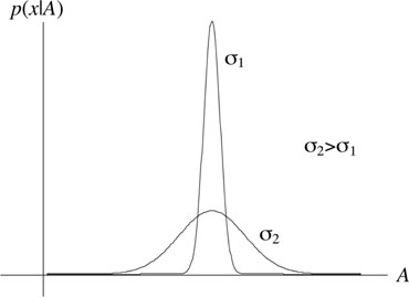
Figure 10.1:  Sharpness of likelihood function and estimation accuracy.

In (10.1), if the noise w is Gaussian with covariance matrix C, then the likelihood function is

$p\left(\text{x}|\mathit{\theta }\right)=\frac{1}{{\left(2\text{π}\right)}^{N/2}{\det }^{1/2}\left[\mathbf{\text{C}}\right]}\exp \left[-\frac{1}{2}{\left(\text{x}-\text{f}\left(\mathit{\theta }\right)\right)}^T{\mathbf{\text{C}}}^{-1}\left(\text{x}-\text{f}\left(\mathit{\theta }\right)\right)\right].$

(10.3)

In likelihood function, x is considered to be fixed, and for different θ, it represents the relative probability that θ being the true parameter (thus the probability that θ generates the given observation x). With this interpretation, one popular method for estimation is the maximum likelihood (ML) estimation approach, which searches for θ that maximizes p(x|θ). We will discuss ML estimation in more detail later in this chapter.

The “sharpness” of the likelihood function contains information about the ultimate accuracy any estimator can achieve. For example, Figure 10.1 shows two likelihood functions for the simple model x = A + w with w being Gaussian with two different variances. It can be seen that the likelihood function with smaller noise variance has a much sharper peak, and the values of A with significant likelihood lie within a small range. Thus, the variance of estimate in this scenario will be smaller. Mathematically, the “sharpness” is quantified by the second order derivative of the likelihood function. This is exactly the idea behind CRLB.

Theorem 10.2.1. (Cramér-Rao Lower Bound) [1] Assume the likelihood function p(x|θ) satisfies the regularity condition

$E\left\{\left[\frac{\partial \ln p\left(\text{x}|\mathit{\theta }\right)}{\partial \theta }\right]\right\}=0$

where the expectation is taken with respect to p(x|θ). Then, the covariance matrix of any unbiased estimator $\widehat{\theta }$ satisfies

$C_{\widehat{\theta }}\ge I^{-1}\left(\theta \right)$

(10.4)

where A ≥ B means A − B is positive semidefinite. Matrix I(θ) is the Fisher information matrix with the (i,j)^th element given by

${\left[I\left(\theta \right)\right]}_{ij}=-E\left\{\left[\frac{{\partial }^2\ln p\left(\text{x}|\theta \right)}{\partial {\theta }_i\partial {\theta }_j}\right]\right\}$

(10.5)

where the expectation is taken with respect to p(x|θ), and θ_i stands for the i^th element of θ.

Equation (10.4) is an inequality on the covariance matrix, which includes as a corollary the lower bound on the variance of individual element-wise estimates: var $\left({\theta }_i\right)={\left[C_{\widehat{\theta }}\right]}_{ii}\ge {\left[I^{-1}\left(\mathit{\theta }\right)\right]}_{ii}$. Also notice that the discussion here is about the potential accuracy, and is irrelevant to the specific estimation method being used. Of course, although the potential ultimate accuracy might be high, using a bad estimator might yield poor performance.

Example 10.2.1. [3] In clock synchronization in a wireless sensor node, the observations can be modeled as

$x_1\left[n\right]={\beta }_1{t}_1\left[n\right]+{\beta }_0+{\beta }_1\left(d+\omega \left[n\right]\right),n=0,\dots ,N-1,$

(10.6)

$x_2\left[n\right]=t_2\left[n\right]/+{\beta }_1-{\beta }_0/{\beta }_1+\left(d+z\left[n\right]\right),n=0,\dots ,N-1,$

(10.7)

where ${\left\{x_{{}_1}\left[n\right],x_2\left[n\right]\right\}}_{n=0}^{N-1}$ are the observations, ${\left\{t_{{}_1}\left[n\right],t_2\left[n\right]\right\}}_{n=0}^{N-1}$ are known quantities and can be considered as the training data, β₁, β₀ and d are the unknowns to be estimated, and w[n] and z[n] are i.i.d. observation noise sequences with zero mean and variance σ².

Since the random delays w[n] and z[n] follow i.i.d. Gaussian distributions, the PDF of the observations conditioned on β₁, β₀ and d can be expressed from (10.6)–(10.7) as ln $p\left({\left\{x_{{}_1}\left[n\right],x_2\left[n\right]\right\}}_{n=0}^{N-1}|{\beta }_1,{\beta }_0,d\right)$

$\begin{array}{l}\ln p\left(\left\{x_1\left[n\right],x_2\left[n\right]\right\}{}_{n=0}^{N-1}|{\beta }_1,{\beta }_0,d\right)\\ =\ln \frac{N}{1\text{π}{\sigma }^{\text{2}}}-\frac{1}{2{\sigma }^2}\times {\displaystyle \sum _{n=0}^{N-1}\left[{\left(\frac{x_1\left[n\right]}{{\beta }_1}-t_1\left[n\right]\frac{{\beta }_0}{{\beta }_1}-d\right)}^2+{\left(x_2\left[n\right]-\frac{t_2\left[n\right]}{{\beta }_1}+\frac{{\beta }_0}{{\beta }_1}-d\right)}^2\right].}\end{array}$

(10.8)

To derive the CRLB, we first check the regularity condition. Taking β₀ as an example, it can be shown that

$\frac{\partial \ln p}{\partial {\beta }_0}=-\frac{1}{{\sigma }^2}{\displaystyle \sum _{n=0}^{N-1}\left[-\frac{1}{{\beta }_1}\left(\frac{x_1\left[n\right]-{\beta }_0}{{\beta }_1}-t_1\left[n\right]-d\right)+\frac{1}{{\beta }_1}\left(x_2\left[n\right]-d-\frac{t_2\left[n\right]-{\beta }_0}{{\beta }_1}\right)\right].}$

(10.9)

Putting (10.6) and (10.7) into (10.9), it yields:

$\frac{\partial \ln p}{\partial {\beta }_0}=-\frac{1}{{\sigma }^2}{\displaystyle \sum _{i=0}^{N-1}\frac{z\left[n\right]-\omega \left[n\right]}{{\beta }_1}}.$

(10.10)

Since w[n] and z[n] have zero means, it is easy to see that the expectation of (10.10) is zero (notice that taking the expectation with respect to x₁[n], x₂[n] is equivalent to taking expectation with respect to w[n], z[n]) and the PDF in (10.8) satisfies the regularity condition for β₀. The regularity conditions for β₁ and d can be checked in a similar way.

From (10.5), the Fisher information matrix is given by

$\text{I}\left({\beta }_1,{\beta }_0,d\right)=\left[\begin{array}{l}-E\left\{\frac{{\partial }^2\ln p}{\partial {\beta }_1^2}\right\}-E\left\{\frac{{\partial }^2\ln p}{\partial {\beta }_1\partial {\beta }_0}\right\}-E\left\{\frac{{\partial }^2\ln p}{\partial {\beta }_1\partial d}\right\}\\ -E\left\{\frac{{\partial }^2\ln p}{\partial {\beta }_0^2}\right\}-E\left\{\frac{{\partial }^2\ln p}{\partial {\beta }_0\partial {\beta }_1}\right\}-E\left\{\frac{{\partial }^2\ln p}{\partial {\beta }_0\partial d}\right\}\\ -E\left\{\frac{{\partial }^2\ln p}{\partial d^2}\right\}-E\left\{\frac{{\partial }^2\ln p}{\partial d\partial {\beta }_1}\right\}-E\left\{\frac{{\partial }^2\ln p}{\partial d\partial {\beta }_0}\right\}\end{array}\right],$

and each element in the matrix can be obtained separately. For example for $-E\left\{\frac{\partial \ln p}{\partial {\beta }_1\partial {\beta }_0}\right\}$, based on (10.9), we obtain

$\frac{{\partial }^2\ln p}{\partial {\beta }_1\partial {\beta }_0}=-\frac{1}{{\sigma }^2}{\displaystyle \sum _{n=0}^{N-1}\left[\frac{2\left(x_1\left[n\right]-2{\beta }_0\right)}{{\beta }_1^3}-\frac{t_1\left[n\right]+x_2\left[n\right]}{{\beta }_1^2}\right]}.$

(10.11)

Putting (10.6) and (10.7) into (10.11), we have

$\frac{{\partial }^2\ln p}{\partial {\beta }_1\partial {\beta }_0}=-\frac{1}{{\sigma }^2}{\displaystyle \sum _{n=0}^{N-1}\left(\frac{t_1\left[n\right]+d+2w\left[n\right]-z\left[n\right]}{{\beta }_1^2}+\frac{t_2\left[n\right]-{\beta }_0}{{\beta }_1^3}\right)}$

(10.12)

Taking expectation of (10.12) with respect to random delays w[n] and z[n] gives

$-E\left\{\frac{{\partial }^2\ln p}{\partial {\beta }_1\partial {\beta }_0}\right\}=\frac{1}{{\sigma }^2{\beta }_1^3}{\displaystyle \sum _{n=0}^{N-1}\left[{\beta }_1\left(t_1\left[n\right]+d\right)+\left(t_2\left[n\right]-{\beta }_0\right)\right],}$

where we have used the fact that w[n] and z[n] have zero means. Similarly, the other elements of I(β₁,β₀,d) can be obtained and the Fisher information matrix can be expressed as

$I\left({\beta }_1,{\beta }_0,d\right)=\frac{1}{{\sigma }^2}\left[\begin{array}{ccc}\mathcal{A}& ℬ& \mathcal{C}\\ ℬ& \frac{2N}{{\beta }_1^2}& 0\\ \mathcal{C}& 0& 2N\end{array}\right],$

(10.13)

where

$\mathcal{A}:={\beta }_1^{-4}{\displaystyle {\sum }_{n=0}^{N-1}\left[{\beta }_1^2{\left(t_1\left[n\right]+d\right)}^2+{\beta }_1^2{\sigma }^2+{\left(t_2\left[n\right]-{\beta }_0\right)}^2\right]}$,

$ℬ:={\beta }_1^{-3}{\displaystyle {\sum }_{n=0}^{N-1}\left[{\beta }_1\left(t_1\left[n\right]+d\right)+\left(t_2\left[n\right]-{\beta }_0\right)\right]}$, and

$\mathcal{C}:={\beta }_1^{-2}{\displaystyle {\sum }_{n=0}^{N-1}\left[{\beta }_1\left(t_1\left[n\right]+d\right)-\left(t_2\left[n\right]-{\beta }_0\right)\right]}$. By inverting the matrix (10.13), it can be shown that the CRLB for each parameter (i.e., the diagonal elements of I⁻¹(β₁,β₀, d)) is given, respectively, by:

$\begin{array}{l}\text{CRLB}\left({\beta }_1\right)=\frac{1N{\sigma }^2}{2N\mathcal{A}-{\beta }_1^2{ℬ}^2-{\mathcal{C}}^2},\\ \text{CRLB}\left({\beta }_0\right)=\frac{{\sigma }^2{\beta }_1^2\left(2N\mathcal{A}-{\mathcal{C}}^2\right)}{2N\left(2N\mathcal{A}-{\beta }_1^2{ℬ}^2-{\mathcal{C}}^2\right)},\\ \text{CRLB}\left(d\right)=\frac{{\sigma }^2\left(2N\mathcal{A}-{\beta }_1^2{ℬ}^2\right)}{2N\left(2N\mathcal{A}-{\beta }_1^2{ℬ}^2-{\mathcal{C}}^2\right)}.\end{array}$

As can be seen from this example, CRLB in general depends on the true parameters.

10.2.2    Finding MVUE Attaining the CRLB

With the lower bound on minimum variance, one may wonder if we can construct an unbiased estimator that can reach the CRLB. The answer is yes. Such an estimator is called efficient and might be obtained during the evaluation of the CRLB.

Theorem 10.2.2. [1] [2] An estimator $\widehat{\mathit{\theta }}=\mathrm{g}\left(\mathrm{x}\right)$ is the MVUE if and only if

$\frac{\partial \ln p\left(\text{x}|\mathit{\theta }\right)}{\partial \mathit{\theta }}=I\left(\mathit{\theta }\right)\left(\text{g}\left(\text{x}\right)-\mathit{\theta }\right)$

(10.14)

for some matrix I(θ). Furthermore, the covariance matrix of the MVUE is I(θ)⁻¹, which is also the CRLB.

Example 10.2.2. [1] Let us consider a linear model

$\text{x}=H\mathit{\theta }+\text{s}+\text{w}$

where x is the observation vector, H represents a known matrix, θ denotes the parameter vector to be estimated, s is a known vector, and w stands for a noise vector with PDF $\mathcal{N}$(0, C). Subtracting s on both sides, and applying the whitening matrix D with D^TD = C⁻¹, we have

$\begin{array}{c}\text{D}\left(\text{x}-\text{s}\right)=\text{D}H\mathit{\theta }+\text{Dw}\\ {\text{x}}^{\prime }\text{=}{\mathbf{\text{H}}}^{\prime }\mathit{\theta }\text{+}{\text{w}}^{\prime }\text{.}\end{array}$

It can be easily shown that w′ is Gaussian with zero mean and the covariance matrix is an identity matrix. Taking the first order derivative of logarithm of the likelihood function in the form of (10.3), it follows that:

$\frac{\partial \ln p\left({\text{x}}^{\prime }|\mathit{\theta }\right)}{\partial \mathit{\theta }}=-\frac{1}{2}\frac{\partial }{\partial \mathit{\theta }}\left[{{\text{x}}^{\prime }}^T{\text{x}}^{\prime }-2{{\text{x}}^{\prime }}^T{\mathbf{\text{H}}}^{\prime }\mathit{\theta }+{\mathit{\theta }}^T{{\mathbf{\text{H}}}^{\prime }}^T\mathbf{\text{H}}\mathit{\theta }\right].$

Since

$\begin{array}{c}\frac{\partial {{\text{x}}^{\prime }}^T{\mathbf{\text{H}}}^{\prime }\mathit{\theta }}{\partial \mathit{\theta }}={{\mathbf{\text{H}}}^{\prime }}^T{\text{x}}^{\prime }\text{,}\\ \frac{\partial {\mathit{\theta }}^T{\mathbf{\text{H}}}^{\prime }\mathit{\theta }}{\partial \mathit{\theta }}=2{{\mathbf{\text{H}}}^{\prime }}^T{\mathbf{\text{H}}}^{\prime }\mathit{\theta }\text{,}\end{array}$

we have

$\begin{array}{l}\frac{\partial \ln p\left({\text{x}}^{\prime }|\mathit{\theta }\right)}{\partial \mathit{\theta }}={{\mathbf{\text{H}}}^{\prime }}^T{\text{x}}^{\prime }-{{\mathbf{\text{H}}}^{\prime }}^T{\mathbf{\text{H}}}^{\prime }\mathit{\theta }\\ ={{\mathbf{\text{H}}}^{\prime }}^T{\mathbf{\text{H}}}^{\prime }\left[{\left({{\mathbf{\text{H}}}^{\prime }}^T{\mathbf{\text{H}}}^{\prime }\right)}^{-1}{{\mathbf{\text{H}}}^{\prime }}^T{\text{x}}^{\prime }-\mathit{\theta }\right],\end{array}$

(10.15)

where in the last step, it is assumed that H^′TH′ is invertible. Comparing the above equation with (10.14), it is obvious that we obtain

$\widehat{\mathit{\theta }}={\left({H^{\prime }}^T{H}^{\prime }\right)}^{-1}{H^{\prime }}^T{\text{x}}^{\prime }={\left(H^T{C}^{-1}H\right)}^{-1}{H}^T{C}^{-1}\left(\text{x}-\text{s}\right),$

(10.16)

$C_{\widehat{\mathit{\theta }}}=I{(\mathit{\theta })}^{-1}=(H{C}^{-1}{H}^{-1}),$

(10.17)

the MVUE and its corresponding covariance, respectively. Notice that this result does not require the computation of second order derivative in order to obtain the CRLB.

10.3    MVUE Using Rao-Blackwell-Lehmann-Scheffe Theorem

In the previous section, we introduced a method for finding MVUE that can reach the CRLB. However, even if there is no estimator that can reach the CRLB, there may still exist a MVUE (the MVUE in such case is not an efficient estimator). In this section, we introduce another technique that can determine the MVUE from the likelihood function, and this technique requires the concept of sufficient statistics.

10.3.1    Sufficient Statistics

In a general estimation problem, we have access to a bunch of observations or data x[0], x[1], …, x[N − 1]. These observations contain information about the parameter we want to estimate. In general, making use of all available data would achieve the best estimation performance (how to use them is another problem). One would wonder: Is there any way to compress the data while the useful information for parameter estimation is not lost? If so, we can compress the original data set into sufficient statistics and use them for parameter estimation instead. Of course, the original data set is a sufficient statistic itself. Furthermore, for given original observations, there are many sufficient statistics. The one with the minimum number of elements is called the minimal sufficient statistic.

Formally, the concept of sufficient statistic is defined as follows. Let x be a vector of observations, and θ be the parameter of interest, with the likelihood function given by p(x|θ). A statistic T(x) is sufficient for θ if p(x|T(x), θ) is independent of θ. Intuitively, if T(x) is observed, and if p(x|T(x), θ) still depends on θ, there must be some information contain in x but not in T(x), and therefore T(x) cannot be a sufficient statistic.

Example 10.3.1. [2] Consider a sequence of independent Bernoulli trial x[0], x[1], …, x[N − 1] ∊ {0,1}. The probability for x[n] = 1 is θ. Then the likelihood function for estimation of θ is

$p\left(\text{x}|\theta \right)={\displaystyle \prod _{n=0}^{N-1}{\theta }^{x\left[n\right]}{\left(1-\theta \right)}^{1-x\left[n\right]}}={\theta }^k{\left(1-\theta \right)}^{N-k}$

(10.18)

where $k:{\displaystyle {\sum }_{n=0}^{N-1}x\left[n\right]}$. Now consider

$p\left(\text{x}|k,\theta \right)=\frac{p\left(\text{x},k|\theta \right)}{p\left(k|\theta \right)}.$

Since κ completely depends on x, p(x, κ|θ) is zero except when κ equals the number of ones in x. When it does, p(x, κ|θ) = p(x|θ). On the other hand, p(κ|θ) is the distribution of number of ones in N independent Bernoulli trials, and it is given by

$p\left(k|\theta \right)=\left(\begin{array}{c}N\\ k\end{array}\right){\theta }^k{\left(1-\theta \right)}^{N-k}.$

Therefore,

$p\left(\text{x}|k,\theta \right)=\frac{{\theta }^k{\left(1-\theta \right)}^{N-k}}{\left(\begin{array}{c}N\\ k\end{array}\right){\theta }^k{\left(1-\theta \right)}^{N-k}}=\frac{1}{\left(\begin{array}{c}N\\ k\end{array}\right)}.$

It is obvious that p(x|κ, θ) is independent of θ, and $k={\displaystyle {\sum }_{n=0}^{N-1}x\left[n\right]}$ is a sufficient statistic. That is, for estimation of θ, we only need to store the number of ones in the observations rather than the original sequence of ones and zeros.

Finding sufficient statistic using the basic definition involves guessing the sufficient statistic and verifying the conditional PDF being independent of the parameter of interest. Both steps can be challenging. Fortunately, we have the following theorem to help us in practice.

Theorem 10.3.1. (Neyman-Fisher Factorization) [1] [2] Let x be a vector of observations with the likelihood function p(x|θ). The statistic T(x) is sufficient if and only if the likelihood function can be factorized as follows

$p(x|\mathit{\theta })=g(T(x),\mathit{\theta })h(x)$

where g is a function depending on x only through T(x) and h is a function depending on x only.

Now, let us revisit the previous example of Bernoulli trials. The likelihood function in (10.18) can be expressed as

$p\left(\text{x}|\theta \right)=\underset{g\left(T\left(\text{x}\right)=k,\theta \right)}{\underbrace{{\theta }^k{\left(1-\theta \right)}^{N-k}}}.\underset{h\left(\text{x}\right)}{\underbrace{1}}.$

The first term g depends on x through κ only, while h is independent of θ. Therefore, from the Neyman-Fisher factorization Theorem, κ is a sufficient statistic. Obviously, identifying the sufficient statistic using this theorem is much simpler. Below is another example.

Example 10.3.2. [1] For the mean estimation from observations x[n] = A + w[n] for n = 0,1,…, N − 1, with w[n] being i.i.d. zero mean Gaussian distributed with variance σ², the likelihood function is given by

$p\left(\text{x}|A\right)=\frac{1}{{\left(2\pi {\sigma }^2\right)}^{N/2}}\exp \left[-\frac{1}{2{\sigma }^2}{\displaystyle \sum _{n=0}^{N-1}{\left(x\left[n\right]-A\right)}^2}\right]$

(10.19)

$=\underset{g\left(T\left(\text{x}\right)={\displaystyle {\sum }_{n=0}^{N-1}x\left[n\right],A}\right)}{\underbrace{\frac{1}{{\left(2\pi {\sigma }^2\right)}^{N/2}}\exp \left[-\frac{1}{2{\sigma }^2}\left(N{A}^2-2A{\displaystyle \sum _{n=0}^{N-1}x\left[n\right]}\right)\right]}}\underset{h\left(\text{x}\right)}{\underbrace{\exp \left[-\frac{1}{2{\sigma }^2}{\displaystyle \sum _{n=0}^{N-1}{x}^2\left[n\right]}\right]}}.$

(10.20)

Now, g depends on x through ${\displaystyle {\sum }_{n=0}^{N-1}x\left[n\right]}$ only, while h is a function of x only and is independent of A. Clearly, $T\left(\mathrm{x}\right)={\displaystyle {\sum }_{n=0}^{N-1}x\left[n\right]}$ is a sufficient statistic for estimating A. Notice that $T^{\prime }\left(\mathrm{x}\right)=2{\displaystyle {\sum }_{n=0}^{N-1}x\left[n\right]}$ is also a sufficient statistic for A. In fact, sufficient statistics are unique only to within a one-to-one transformation.

□

Another concept that is important to the determination of MVUE is the concept of complete sufficient statistic. In essence, a statistic is complete if there is only one function of the statistic that forms an unbiased estimator. Suppose T(x) is a sufficient statistic for θ. Furthermore, suppose there are two function g₁ and g₂ of T (x) that are unbiased estimators of θ. Equivalently, we have

$E\{g_1(T(\text{x}))-g_2(T(\text{x}))\}=0$

(10.21)

for all θ, and the expectation is taken with respect to the observations (or equivalently the sufficient statistics). In order to prove T(x) is a complete sufficient statistic, we must prove that if (10.21) holds, then g₁(T(x)) = g₂(T(x)).

Example 10.3.3. [1] In the estimation of A from observations x[n] = A + w[n] with w[n] being i.i.d. Gaussian noise with zero mean and variance σ², we have shown in the previous example that a sufficient statistic for A is $T\left(\mathrm{x}\right)={\displaystyle {\sum }_{n=0}^{N-1}x\left[n\right]}$. Now suppose there are two unbiased estimators g₁(T(x)) and g₂(T(x)), that is

$E\left\{g_1\left(T\left(\text{x}\right)\right)-g_2\left(T\left(\text{x}\right)\right)\right\}=0$

for all A. Since τ ≔ T(x) ~ $\mathcal{N}$(NA, Nσ²), and defining v(τ) ≔ g₁(τ) − g₂(τ), the above equation is equivalent to

${\displaystyle {\int }_{-\infty }^{\infty }v\left(\tau \right)\frac{1}{\sqrt{2\pi N{\sigma }^2}}\exp \left[-\frac{1}{2N{\sigma }^2}{\left(NA-\tau \right)}^2\right]dr=0.}$

It can be recognized that the above equation is the convolution of v(τ) and a Gaussian pulse. Since the Gaussian pulse is non-negative, in order to have the convolution equal to zero for all A, v(τ) must be identically zero. Therefore, g₁(T(x)) = g₂(T(x)), implying the unbiased estimator is unique, and the sufficient statistic $T\left(\mathrm{x}\right)={\displaystyle {\sum }_{n=0}^{N-1}x\left[n\right]}$ is complete.

□

10.3.2    Finding MVUE from Sufficient Statistics

With the background of sufficient statistics, we now present a theorem that helps us to identify the MVUE.

Theorem 10.3.2. (Rao-Blackwell-Lehmann-Scheffe) [1] [2] Let $\widehat{\theta }$ be an unbiased estimator of θ, and T(x) be a sufficient statistic for θ. Then $\widehat{\theta }=E\left\{\widehat{\theta }|{\rm T}\left(\mathrm{x}\right)\right\}$ improves on $\stackrel{⌣}{\theta }$ in the following ways:

1.  $\widehat{\theta }$ is a valid unbiased estimator for θ;

2.  var $\left(\widehat{\theta }\right)\le \mathrm{var}\left(\stackrel{⌣}{\theta }\right)$.

The result of this theorem is important in the sense that it provides a way to improve the variance of any unbiased estimator using sufficient statistics. However, this theorem does not immediately offer the MVUE, since it is not guaranteed that the improved estimator is of minimum variance within the class of unbiased estimators. But if we have the additional knowledge that the sufficient statistic is complete, the estimator $\widehat{\theta }=E\left\{\stackrel{⌣}{\theta }|T\left(x\right)\right\}$ is the only unbiased estimator for θ while making use of the sufficient statistic. Therefore, it must be the MVUE. In fact, if the estimator we start with $\stackrel{⌣}{\theta }$ is also an unbiased estimator using complete sufficient statistics, it is automatically the MVUE, since there is only one unbiased estimator if the sufficient statistic is complete. There is even no need to compute the expectation $E\left\{\stackrel{⌣}{\theta }|T\left(x\right)\right\}$. In summary, the procedure of determining MVUE using Rao-Blackwell-Lehmann-Scheffe theorem is as follows.

1.  Find a sufficient statistic for θ, T(x), using Neyman-Fisher factorization Theorem.

2.  Determine if the sufficient statistic is complete.

3.  If so, find a function $\widehat{\theta }=\mathrm{g}\left(T\left(x\right)\right)$ which is an unbiased estimator of θ. The MVUE will be $\widehat{\theta }$.

Example 10.3.4. [4] In the clock offset estimation in a wireless sensor node, the observation equations can be written as

$\begin{array}{cccc}{U}_n& =& \delta +\varphi +w_n,& n=1,2,\dots ,N,\\ V_n& =& \delta -\varphi +z_n,& n=1,2,\dots N,\end{array}$

where δ symbolizes the fixed portions of the transmission delays, w_n and z_n denote the variable portions of delays and assume i.i.d. exponential distributions with means α and β, respectively, and φ stands for the clock phase offset from the reference time. We want to determine the MVUE of θ ≔ [δ, ϕ, α, β]^T using the procedure introduced above.

First, we need to determine a sufficient statistic. The likelihood of θ is given by

$\begin{array}{l}L\left(\theta \right)=\underset{:=g_1\left({\displaystyle {\sum }_{n=1}^N{U}_n,\delta ,\varphi ,\alpha }\right)}{\underbrace{{\alpha }^{-N}{e}^{-\frac{1}{\alpha }{\displaystyle \sum _{n=1}^N\left(U_n-\delta -\varphi \right)}}}}\underset{:=g_3\left(U_{\left(1\right)},\delta ,\varphi \right)}{\underbrace{u\left[U_{\left(1\right)}-\delta -\varphi \right]}}.\\ \underset{:=g_2\left({\displaystyle {\sum }_{n=1}^N{V}_n,\delta ,\varphi ,\alpha }\right)}{\underbrace{{\beta }^{-N}{e}^{-\frac{1}{\beta }{\displaystyle \sum _{k=1}^N\left(V_k-\delta +\varphi \right)}}}}\underset{:=g_4\left(V_{\left(1\right)},\delta ,\varphi \right)}{\underbrace{u\left[V_{\left(1\right)}-\delta +\varphi \right]}}.\underset{:=h\left(U_n,V_n\right)}{\underbrace{1}},\end{array}$

where u[·] denotes the unit step function, and U₍₁₎ and V₍₁₎ are the minimum order statistics of U_κ and V_κ, respectively. In the above expression, h(U_n, V_n) is independent of the unknown parameter vector θ, whereas g₁, g₂, g₃ and g₄ are functions depending on the data through $T=\left\{{\displaystyle {\sum }_{n=1}^N{U}_n,U_{\left(1\right)}},{\displaystyle {\sum }_{n=1}^N{V}_n},V_{\left(1\right)}\right\}$. Therefore, according to Neyman-Fisher factorization Theorem 10.3.1, T is a sufficient statistic for θ.

Next, we need to prove that T is complete, a step which requires the PDF of T. Unfortunately, since ${\displaystyle {\sum }_{n=1}^N{U}_n}$ and U₍₁₎, and similarly ${\displaystyle {\sum }_{n=1}^N{V}_n}$ and V₍₁₎, are not independent, the PDF of T is difficult to be obtained. But if we consider the statistic $T^{\prime }=\left\{{\displaystyle {\sum }_{n=1}^N\left(U_n-U_{\left(1\right)}\right),U_{\left(1\right)}},{\displaystyle {\sum }_{n=1}^N\left(V_n-V_{\left(1\right)}\right)},V_{\left(1\right)}\right\}$, it turns out that it is also a sufficient statistic because it is obtained using a one-to-one transformation from T. It can be proved that the elements of T′ are independent, and each of them obeys the three-parameter Gamma distribution:

$\begin{array}{rrrrr}\hfill r& \hfill :=& \hfill {\displaystyle \sum _{n=1}^N\left(U_n-U_{\left(1\right)}\right)}& \hfill \sim & \Gamma \left(N-1,\alpha ,0\right),\hfill \\ \hfill s& \hfill :=& \hfill {\displaystyle \sum _{n=1}^N\left(V_n-V_{\left(1\right)}\right)}& \hfill \sim & \Gamma \left(N-1,\beta ,0\right),\hfill \\ \hfill & \hfill & \hfill U_{\left(1\right)}& \hfill \sim & \Gamma \left(1,\alpha /N,\delta +\varphi \right),\hfill \\ \hfill & \hfill & \hfill V_{\left(1\right)}& \hfill \sim & \Gamma \left(1,\beta /N,\delta -\varphi \right).\hfill \end{array}$

Now, suppose there are two functions g(T′) and h(T′) that are unbiased estimators of θ. Then we have

$\begin{array}{cc}E\left\{g\left({\mathbf{\text{T}}}^{\prime }\right)-h\left({\mathbf{\text{T}}}^{\prime }\right)\right\}=E\left\{\pi \left({\mathbf{\text{T}}}^{\prime }\right)\right\}=0& \forall \theta \end{array}$

where π(T′) ≔ g(T′) − h(T′). As a result,

$\begin{array}{l}{\displaystyle {\int }_{\delta -\varphi }^{\infty }{\displaystyle {\int }_0^{\infty }{\displaystyle {\int }_{\delta +\varphi }^{\infty }{\displaystyle {\int }_0^{\infty }\pi \left(r,U_{\left(1\right)},s,V_{\left(1\right)}\right).\frac{{\left(\alpha \beta \right)}^{-\left(N-1\right)}}{{\left\{\Gamma \left(N-1\right)\right\}}^2}{\left(rs\right)}^{N-2}{e}^{-\frac{r}{\alpha }-\frac{s}{\beta }}}}}}\\ \times \frac{N^2}{\alpha \beta }{e}^{-\frac{N}{\alpha }\left\{U_{\left(1\right)}-\delta -\varphi \right\}-\frac{N}{\beta }\left\{V_{\left(1\right)}-\delta +\varphi \right\}}drd{U}_{\left(1\right)}dsd{V}_{\left(1\right)}=0\end{array}$

for all θ. The above relation can also be expressed as

$\begin{array}{l}{\displaystyle {\int }_{-\infty }^{\infty }{\displaystyle {\int }_{-\infty }^{\infty }{\displaystyle {\int }_{-\infty }^{\infty }{\displaystyle {\int }_{-\infty }^{\infty }\left[\pi \left(r,U_{\left(1\right)},s,V_{\left(1\right)}\right){\left(rs\right)}^{N-2}u\left(s\right)u\left(r\right)u\left(U_{\left(1\right)}-\delta -\varphi \right)u\left(V_{\left(1\right)}-\delta +\varphi \right)\right]}}}}\\ \times e^{-\left\{\frac{r}{\alpha }+\frac{N{U}_{\left(1\right)}}{\alpha }+\frac{s}{\beta }+\frac{N{V}_{\left(1\right)}}{\beta }\right\}}drd{U}_{\left(1\right)}dsd{V}_{\left(1\right)}=0.\end{array}$

The expression on the left above is the four-dimensional Laplace transform of the function within the square brackets. It follows from the uniqueness theorem for the two-sided Laplace transform that π(T′)(rs)^N−2u(s)u(r)u(U₍₁₎ − δ − ϕ)u(V₍₁₎ − δ + ϕ) = 0 almost everywhere. Since r, s, u(s), u(r), u(U₍₁₎ − δ − ϕ), u(V₍₁₎ − δ + ϕ) are not identically zero, we can conclude that π(T′) = 0, resulting in g(T′) = h(T′). This proves that the statistic T′, or equivalently T, is complete for estimating θ.

Finally, we have to find an unbiased estimator for θ as a function of T. A careful inspection of the sufficient statistics reveals that

$\widehat{\theta }=\frac{1}{2\left(N-1\right)}\left[\begin{array}{c}N\left(U_{\left(1\right)}+V_{\left(1\right)}\right)-\frac{1}{N}\left({\displaystyle {\sum }_{n=1}^N{U}_n+{\displaystyle {\sum }_{n=1}^N{V}_n}}\right)\\ N\left(U_{\left(1\right)}-V_{\left(1\right)}\right)-\frac{1}{N}\left({\displaystyle {\sum }_{n=1}^N{U}_n-{\displaystyle {\sum }_{n=1}^N{V}_n}}\right)\\ 2N\left(\frac{1}{N}{\displaystyle {\sum }_{n=1}^N{U}_n-U_{\left(1\right)}}\right)\\ 2N\left(\frac{1}{N}{\displaystyle {\sum }_{n=1}^N{V}_n-V_{\left(1\right)}}\right)\end{array}\right]$

is an unbiased estimator of θ, which is also the MVUE according to the Rao-Blackwell-Lehmann-Scheffe Theorem 10.3.2.

10.4    Maximum Likelihood Estimation

In general, determining MVUE is difficult due to the fact that we do not know whether the MVUE for a particular problem exists. Even if it does exist, the procedure for determining the MVUE is overwhelmingly challenging for most problems. Therefore, in practice, MVUEs are only reported in isolated cases. In this section, we introduce the maximum likelihood (ML) estimation, a popular technique that usually results in practical estimators.

10.4.1    ML Estimation Principle

As it was introduced previously in Section 10.2 in the context of Cramér-Rao lower bound, the likelihood function can be interpreted as a PDF of the unknown parameter θ with fixed observation x. The maximum likelihood estimation approach resumes to finding the parameter vector that maximizes the likelihood function:

$\widehat{\theta }=\arg \left[\underset{\tilde{\theta }}{\max }p\left(\text{x}|\tilde{\theta }\right)\right],$

where $\tilde{\theta }$ is the trial value of the unknown parameter. In fact, the ML estimate $\widehat{\theta }$ is the parameter that is the most probable for generating the observations.

Example 10.4.1. [1] Consider the received data x[n] = A + w[n] for n = 0,1,…, N − 1, with A unknown, and w[n] is i.i.d. Gaussian distributed with zero mean and variance σ². We want to derive the ML estimator for A. First, the likelihood function of A is given by (10.19). Taking logarithm on the likelihood function gives

$\ln p\left(\text{x}|A\right)=-\frac{N}{2}\ln 2\pi -N\ln \sigma -\frac{1}{2{\sigma }^2}{\displaystyle \sum _{n=0}^{N-1}{\left(x\left[n\right]-A\right)}^2.}$

Since the value of A that maximizes p(x|A) is the same as that maximizing ln p(x|A), we can proceed to maximize the log-likelihood function ln p(x|A) instead. Differentiating ln p(x|A) with respect to A, we have

$\frac{\partial \ln p\left(\text{x}|A\right)}{\partial A}=\frac{1}{{\sigma }^2}{\displaystyle \sum _{n=0}^{N-1}\left(x\left[n\right]-A\right).}$

(10.22)

Setting (10.22) to zero, the ML estimator of A is given by

$\widehat{A}=\frac{1}{N}{\displaystyle \sum _{n=0}^{N-1}x\left[n\right],}$

which can be interpreted as the sample mean estimator.

Notice that the first derivative of the log-likelihood function (10.22) of the above example can also be written as

$\frac{\partial \ln p\left(\text{x}|A\right)}{\partial A}=\frac{N}{{\sigma }^2}\left(\frac{1}{N}{\displaystyle \sum _{n=0}^{N-1}x\left[n\right]-A}\right).$

(10.23)

Comparing (10.23) to (10.14), it is obvious that the ML estimator of A is also the MVUE. Furthermore, in the general linear model considered in Example 10.2.2, the first derivative of the log-likelihood function is given by (10.15). By setting (10.15) to zero and solving for θ, the ML estimator of θ can be easily shown to be identical to the MVUE in (10.16). This can be viewed as a special case of following important result.

Theorem 10.4.1. (Optimality of the MLE for the Linear Model) [1] [2] For the data x described by the general linear model

$\text{x}=H\theta +\text{w}$

where H stands for a known N × p matrix with N > p and of full rank, θ represents a p × 1 vector of parameters to be estimated, and w denotes the Gaussian noise vector with PDF $\mathcal{N}$(0, C), the ML estimate of θ is given by

$\widehat{\theta }={(H^T{C}^{-1}H)}^{-1}{H}^T{C}^{-1}\text{x}.$

(10.24)

Furthermore, $\widehat{\theta }$ is also the MVUE and its variance (H^TC⁻¹H)⁻¹ attains the CRLB.

The above two examples are not pure coincidence. In fact, if an unbiased estimator attains the CRLB (i.e., an efficient estimator exists), the ML procedure will produce it. This can be easily explained by the fact that if an efficient estimator exists, (10.14) holds. On the other hand, ML estimate is obtained by setting the first derivative of the log-likelihood function, i.e., (10.14), to zero. This automatically produces $\widehat{\theta }=\mathrm{g}\left(x\right)$, which is also the MVUE.

10.4.2    Properties of the ML Estimator

However, being identical to the MVUE in certain situations is not the main reason for the popularity of the ML estimation, as these situations do not frequently occur. On the other hand, the following property itself is strong enough for the ML estimation to be useful in practice.

Theorem 10.4.2. (Asymptotic Property of the ML estimator) [1] [2] If the likelihood function p(x|θ) of data x satisfies certain “regularity” conditions (existence of the derivatives of the log-likelihood function, as well as the Fisher information being nonzero), then the ML estimate of θ is asymptotically distributed (for large data records) according to

$\widehat{\theta }\underset{˜}{a}\mathcal{N}(\theta ,I^{-1}(\theta ))$

where I(θ) is the Fisher information matrix evaluated at the true value of the unknown parameter.

This theorem states that when the observation data length tends to infinity, the ML estimate is asymptotically unbiased and asymptotically attains the CRLB. The ML estimate is therefore asymptotically efficient.

Example 10.4.2. [1] Consider x[n] = A + w[n] for n = 0,1,…,N − 1, with A > 0 is the parameter of interest, and w[n] is i.i.d. Gaussian noise with unknown variance A. The likelihood function of A is

$p\left(x|A\right)=\frac{1}{{\left(2\pi A\right)}^{N/2}}\exp \left[-\frac{1}{2A}{\displaystyle \sum _{n=0}^{N-1}{\left(x\left[n\right]-A\right)}^2}\right].$

Notice that this problem is not the same as that in the last example, as A appears as both the mean of received data and the variance of the noise. Differentiating the log-likelihood function with respect to A, it follows that

$\frac{\partial \ln p\left(\text{x}|A\right)}{\partial A}=-\frac{N}{2A}+\frac{1}{A}{\displaystyle \sum _{n=0}^{N-1}\left(x\left[n\right]-A\right)+\frac{1}{2A^2}{\displaystyle \sum _{n=0}^{N-1}{\left(x\left[n\right]-A\right)}^2.}}$

(10.25)

Setting the result to zero produces

$A^2+A-\frac{1}{N}{\displaystyle \sum _{n=0}^{N-1}{x}^2\left[n\right]=0,}$

which yields the ML estimate of A:

$\widehat{A}=-\frac{1}{2}+\sqrt{\frac{1}{N}{\displaystyle \sum _{n=0}^{N-1}{x}^2\left[n\right]+\frac{1}{4},}}$

and the other solution is dropped to guarantee A > 0.

Now, we will examine the asymptotic mean and variance of the above estimator. To simply the notation, we let $u=\frac{1}{N}{\displaystyle {\sum }_{n=0}^{N-1}{x}^2\left[n\right]}$, and g(u) be the function:

$\widehat{A}=g\left(u\right)=-\frac{1}{2}+\sqrt{u+\frac{1}{4}}.$

As N → ∞, u → E {x²[n]} = A² + A := u_o. Using a first order Taylor series approximation for g(u) around u_o yields

$\begin{array}{c}\widehat{A}=g\left(u\right)\approx g\left(u_o\right)+\frac{dg\left(u\right)}{du}|{}_{u=u_o}\left(u-u_o\right)\\ =A+\frac{1/2}{A+1/2}\left[\frac{1}{N}{\displaystyle \sum _{n=0}^{N-1}{x}^2\left[n\right]-\left(A+A^2\right)}\right].\end{array}$

Therefore, E {Â} = A, so  is asymptotically unbiased. Furthermore, the asymptotic variance is computed as

$\begin{array}{c}\mathrm{var}\left(\widehat{A}\right)={\left(\frac{1/2}{A+1/2}\right)}^2\mathrm{var}\left(\frac{1}{N}{\displaystyle \sum _{n=0}^{N-1}{x}^2\left[n\right]}\right)\\ =\frac{1/4}{N{\left(A+1/2\right)}^2}\mathrm{var}\left(x^2\left[n\right]\right).\end{array}$

Since x[n] is Gaussian distributed with mean A and variance A, it can be shown that var (x²[n]) = 4A³ + 2A², and therefore

$\mathrm{var}\left(\widehat{A}\right)=\frac{A^2}{N\left(A+1/2\right)}.$

(10.26)

To check whether this asymptotic variance equals the CRLB, we differentiate (10.25) with respect to A again, and obtain

$\frac{\partial \ln p\left(\text{x}|A\right)}{\partial A^2}=\frac{N}{2A^2}-\frac{1}{A^2}{\displaystyle \sum _{n=0}^{N-1}\left(x\left[n\right]-A\right)-\frac{N}{A}-\frac{1}{A^3}{\displaystyle \sum _{n=0}^{N-1}{\left(x\left[n\right]-A\right)}^2{\displaystyle \sum _{n=0}^{N-1}\left(x\left[n\right]-A\right).}}}$

The CRLB of A is then given by

$\begin{array}{c}{\left[-E\left\{\frac{{\partial }^2\ln p\left(\text{x}|A\right)}{\partial A^2}\right\}\right]}^{-1}=-{\left(\frac{N}{2A^2}-\frac{N}{A}-\frac{N}{A^2}\right)}^{-1}\\ =\frac{A^2}{N\left(A+1/2\right)}.\end{array}$

The asymptotic variance (10.26) coincides with the CRLB. Therefore, the ML estimator for A is asymptotic efficient.

□

Example 10.4.3. [5] In orthogonal frequency division multiple access (OFDMA) uplink, multiple signals from different users arrive at the base station at the same time. However, their carrier frequency offsets (CFO) and channels are different and unknown. Before the data can be detected, we need to estimate all these parameters. In general, the received signal model in such systems can be expressed in the form of matrix equation:

$\text{x}=\mathbf{\text{Q}}\left(\mathbf{\omega }\right)\mathbf{\text{h}}+\text{w},$

(10.27)

where x stands for the received data from one OFDM symbol, h denotes an unknown vector containing the channel coefficients of different users, Q(ω) is a matrix with known structure but parameterized nonlinearly by the unknown vector ω = [ω₁ ω₂ …ω_K]^T of frequency offsets, w represents the i.i.d. complex Gaussian noise with zero mean and variance σ². The ML estimate of parameters {h, ω} is obtained by maximizing the likelihood function

$p\left(\text{x}|\widetilde{\mathbf{\text{h}}},\tilde{\mathbf{\omega }}\right)=\frac{1}{{\left(\pi {\sigma }^2\right)}^N}\cdot \exp \left\{-\frac{1}{{\sigma }^2}{\left[\text{x}-\mathbf{\text{Q}}\left(\tilde{\mathbf{\omega }}\right)\widetilde{\mathbf{\text{h}}}\right]}^H\left[\text{x}-\mathbf{\text{Q}}\left(\tilde{\mathbf{\omega }}\right)\widetilde{\mathbf{\text{h}}}\right]\right\},$

(10.28)

where h̃ and $\tilde{\mathbf{\omega }}$ are trial values of h and ω, respectively. Notice that since w is complex, the PDF expression (10.28) assumes a slightly different form than that when w is real-valued in (10.3). Taking the logarithm of (10.28), and ignoring the constant irrelevant terms, the ML estimate can be equivalently found by minimizing

$\Lambda \left(\text{x}|\widetilde{\mathbf{\text{h}}},\tilde{\mathbf{\omega }}\right)={\left[\text{x}-\mathbf{\text{Q}}\left(\tilde{\mathbf{\omega }}\right)\widetilde{\mathbf{\text{h}}}\right]}^H\left[\text{x}-\mathbf{\text{Q}}\left(\tilde{\mathbf{\omega }}\right)\widetilde{\mathbf{\text{h}}}\right].$

(10.29)

Due to the linear dependence of parameter h in (10.27), the ML estimate for the channel vector h (when $\tilde{\mathbf{\omega }}$ is fixed) is given by (see (10.24))

$\widehat{\mathbf{\text{h}}}=({\mathbf{\text{Q}}}^H\left(\tilde{\mathbf{\omega }}\right)\mathbf{\text{Q}}{\left(\tilde{\mathbf{\omega }}\right))}^{-1}{\mathbf{\text{Q}}}^H\left(\tilde{\mathbf{\omega }}\right)\text{x}.$

Plugging ĥ into (10.29), and retaining only those terms related to $\tilde{\mathbf{\omega }}$, the ML estimate of ω can be expressed as

$\widehat{\mathbf{\omega }}=\arg \underset{\tilde{\mathbf{\omega }}}{\max }\left\{J\left(\tilde{\mathbf{\omega }}\right):={\text{x}}^H\mathbf{\text{Q}}\left(\tilde{\mathbf{\omega }}\right){\left({\mathbf{\text{Q}}}^H\left(\tilde{\mathbf{\omega }}\right)\mathbf{\text{Q}}\left(\tilde{\mathbf{\omega }}\right)\right)}^{-1}{\mathbf{\text{Q}}}^H\left(\tilde{\mathbf{\omega }}\right)\text{x}\right\}.$

(10.30)

Now the question resumes to how to maximize the nonlinear function $J\left(\tilde{\mathbf{\omega }}\right)$. One straightforward way is to use a grid search, in which the feasible region of the parameter is divided into many subregions and the potential points are checked one by one. For example, if the parameter ω is one-dimensional and lies within [a, b], we can divide this range into 10,000 equally spaced intervals, and compute the cost function for 10,000 different values of ω. This approach may be acceptable in the presence of a single unknown parameter. However, when the dimension of parameter vector increases, the number of points to be searched increases exponentially. For example, if there are four users in the OFDMA system, the unknown vector ω is four dimensional. If we divide each dimension into 10,000 subintervals, the number of points to be searched is (10,000)⁴. This is unacceptable. Furthermore, if the parameter of interest is not bounded to a finite-length interval, this approach is also practically infeasible.

Another possible solution is to use iterative numerical search methods, such as the Newton-Raphson or steepest descent method. The idea is to approximate the optimization of a nonlinear function by a series of linearized optimizations with respect to a previously obtained solution. In the Newton-Raphson method, the second order Taylor series expansion is applied to the nonlinear function J(ω) around a previous estimate ${\tilde{\mathbf{\omega }}}^{\left(i\right)}$:

$J\left(\mathbf{\omega }\right)\approx J\left({\widehat{\mathbf{\omega }}}^{\left(i\right)}\right)+\left(\mathbf{\omega }-{\widehat{\mathbf{\omega }}}^{\left(i\right)}\right)\frac{\partial J\left(\mathbf{\omega }\right)}{\partial \mathbf{\omega }}|{}_{\mathbf{\omega }={\widehat{\mathbf{\omega }}}^{\left(i\right)}}+\frac{1}{2}{\left(\mathbf{\omega }-{\widehat{\mathbf{\omega }}}^{\left(i\right)}\right)}^H{\left[\frac{{\partial }^{2}J\left(\mathbf{\omega }\right)}{\partial \mathbf{\omega }\partial {\mathbf{\omega }}^H}\right]}_{\mathbf{\omega }={\widehat{\mathbf{\omega }}}^{\left(i\right)}}\left(\mathbf{\omega }-{\widehat{\mathbf{\omega }}}^{\left(i\right)}\right)$

(10.31)

where

$\frac{\partial J\left(\mathbf{\omega }\right)}{\partial \mathbf{\omega }}={\left[\frac{\partial J}{\partial {\omega }_1},\frac{\partial J}{\partial {\omega }_2},\dots .\frac{\partial J}{\partial {\omega }_K}\right]}^T$

is the gradient vector, and

$\frac{{\partial }^{2}J\left(\mathbf{\omega }\right)}{\partial \mathbf{\omega }\partial {\mathbf{\omega }}^H}=\left(\begin{array}{cccc}\frac{{\partial }^{2}J}{\partial {\mathbf{\omega }}_1\partial {\omega }_1}& \frac{{\partial }^{2}J}{\partial {\omega }_1\partial {\omega }_2}& \cdots & \frac{{\partial }^{2}J}{\partial {\omega }_1\partial {\omega }_K}\\ \frac{{\partial }^{2}J}{\partial {\omega }_2\partial {\omega }_1}& \frac{{\partial }^{2}J}{\partial {\omega }_2\partial {\omega }_2}& \cdots & \frac{{\partial }^{2}J}{\partial {\omega }_2\partial {\omega }_K}\\ ⋮& & & \\ \frac{{\partial }^{2}J}{\partial {\omega }_K\partial {\omega }_1}& \frac{{\partial }^{2}J}{\partial {\omega }_K\partial {\omega }_2}& \cdots & \frac{{\partial }^{2}J}{\partial {\omega }_K\partial {\omega }_K}\end{array}\right)$

is the Hessian of J(ω). Differentiating (10.31) with respect to $\left(\mathbf{\omega }-{\widehat{\mathbf{\omega }}}^{\left(i\right)}\right)$ and setting the result to zero leads to

$\frac{\partial J\left(\mathbf{\omega }\right)}{\partial \mathbf{\omega }}|{}_{\mathbf{\omega }={\widehat{\mathbf{\omega }}}^{\left(i\right)}}+{\left[\frac{\partial 2J\left(\mathbf{\omega }\right)}{\partial \mathbf{\omega }\partial {\mathbf{\omega }}^H}\right]}_{\mathbf{\omega }={\widehat{\mathbf{\omega }}}^{\left(i\right)}}\left(\mathbf{\omega }={\widehat{\mathbf{\omega }}}^{\left(i\right)}\right)=0.$

Solving the above equation gives the value of ω that maximizes the second order approximated Taylor series expansion:

${\widehat{\mathbf{\omega }}}^{\left(i+1\right)}={\widehat{\mathbf{\omega }}}^{\left(i\right)}-{\left[\frac{{\partial }^{2}J\left(\mathbf{\omega }\right)}{\partial \mathbf{\omega }\partial {\mathbf{\omega }}^H}\right]}_{\mathbf{\omega }={\widehat{\mathbf{\omega }}}^{\left(i\right)}}^{-1}\frac{\partial J\left(\mathbf{\omega }\right)}{\partial \mathbf{\omega }}|{}_{\mathbf{\omega }={\widehat{\mathbf{\omega }}}^{\left(i\right)}}.$

On the other hand, in the steepest descent method, the update is given by the equation:

${\widehat{\mathbf{\omega }}}^{\left(i+1\right)}={\widehat{\mathbf{\omega }}}^{\left(i\right)}-\alpha \frac{\partial J\left(\mathbf{\omega }\right)}{\partial \mathbf{\omega }}|{}_{\mathbf{\omega }={\widehat{\mathbf{\omega }}}^{\left(i\right)}},$

where ${\widehat{\mathbf{\omega }}}^{\left(i\right)}$ is the estimate of ω at the i^th iteration, the gradient vector ∂J(ω)/∂ω points in the direction of the maximum increase of J(ω) at the point ω, and α is a parameter that determines how far away each update moves along the direction opposite to the gradient. Notice that the steepest descent method is derived to minimize a function, but minimizing a function is equivalent to maximizing the negative of the same function. Therefore, we do not explicitly describe the maximization algorithm.

Both methods share some similarities. For example, both methods require the initial estimate near the global optimal solution. Otherwise, in general, in the presence of multi-modal objective functions, only convergence to a local optimum can be guaranteed. Furthermore, both methods require the use of the derivative information. However, the Newton-Raphson method requires the additional computation of the Hessian, which may be difficult or impossible to obtain. Notice that even if the Hessian can be obtained, it may not be invertible. However, the use of the Hessian information (if available) ensures a faster convergence rate for the Newton-Raphson method relative to the steepest descent method.

Newton-Raphson and steepest descent methods may indeed reduce the computational complexity compared to the grid search. However, they are still multidimensional optimization approaches. To further reduce the computational burden brought by the multidimensional searches in the ML estimator, the alternating projection algorithm can be exploited. The alternating projection method reduces a K-dimensional maximization problem (10.30) into a series of one-dimensional maximization problems, by updating one parameter at a time, while keeping the other parameters fixed at the previous estimated values. Let ${\widehat{\mathbf{\omega }}}_k^{\left(i\right)}$ be the estimate of ω_κ at the i^th iteration. Further, let

${\widehat{\mathbf{\omega }}}_{-k}^{\left(i\right)}={\left[{\widehat{\omega }}_1^{\left(i+1\right)}\cdots {\widehat{\omega }}_{k-1}^{\left(i+1\right)}{\widehat{\omega }}_{k+1}^{\left(i\right)}\cdots {\widehat{\omega }}_{k+1}^{\left(i\right)}\right]}^T.$

Given the initial estimates ${\left\{{\widehat{\mathbf{\omega }}}_k^{\left(0\right)}\right\}}_{k=0}^K$, the i^th (i ≥ 1) iteration of the alternating projection algorithm for maximizing (10.30) assumes the following form:

${\widehat{\mathbf{\omega }}}_k^{\left(i\right)}=\arg \underset{{\tilde{\mathbf{\omega }}}_k}{\max }\left\{J\left({\tilde{\mathbf{\omega }}}_k,{\widehat{\mathbf{\omega }}}_{-k}^{\left(i-1\right)}\right)\right\},$

for κ = 1,…,K. Grid search, steepest descent or Newton-Raphson method can be used in each of the one-dimensional search. Multiple iterations on i are performed until the estimates of ω_κ converge to a stable solution. Similar to other iterative algorithms, in general, the alternating projection can only be guaranteed to converge to at least a local optimum. Therefore, a good initialization is important.

Figure 10.2(a) shows the MSE performance of the ML estimator of ω with alternating projection and grid search in each dimension, as a function of observation length N. There are two users (K=2), the signal–to–noise ratio (SNR) is set to 10dB, and the number of iterations for alternating projection is 3. CRLB is also shown in the figure. It can be seen that the performance of the ML estimator approaches the CRLB when N increases, confirming the ML estimator is asymptotic efficient. On the other hand, Figure 10.2(b) shows the MSE performance of the ML estimator as a function of SNR. The OFDMA system has N = 64 subcarriers and K = 4 users. It is obvious that the MSE coincides with the CRLB in medium to high SNRs. Notice that increasing the number of observations has the same effect as decreasing the noise variance in observations. Thus, the ML estimator is also asymptotically efficient at high SNRs.

The ML estimate of a parameter θ is obtained by maximizing the likelihood function p(x|θ). But suppose we are interested not in θ itself, but α = g(θ). The question is if we can obtain the ML estimate of α from the ML estimate of θ. Such a situation occurs when the ML estimate of θ is relatively easy to obtain, but the direct derivation of ML estimate of α is difficult. The following theorem answers this question and is another major factor in making the ML estimation so popular.

Theorem 10.4.3. (Invariance property of the ML estimator) [1] Suppose α = g(θ); where θ is a p × 1 vector with likelihood function p(x|θ) and g is an r-dimensional function of θ. The ML estimator of α is given by

$\widehat{\alpha }=\text{g}\left(\widehat{\theta }\right)$

where $\widehat{\theta }$ is the ML estimate of θ.

Example 10.4.4. In this example, we consider again the clock synchronization of wireless sensor node discussed in Example 10.2.1, with observations given by (10.6) and (10.7). However, in this example, the observation noise w[n] and z[n] are modeled as i.i.d. exponential random variables with an unknown common rate parameter λ. The goal is to estimate β₀, β₁, λ and d based on the observations ${\left\{x_1\left[n\right],x_2\left[n\right]\right\}}_{n=0}^{N-1}$.

To derive the ML estimator, we rewrite the observation equations (10.6) and (10.7) as

$w\left[n\right]=\frac{1}{{\beta }_1}\cdot x_1\left[n\right]-t_1\left[n\right]-\frac{{\beta }_0}{{\beta }_1}-d,$

(10.32)

$z\left[n\right]=-\frac{1}{{\beta }_1}\cdot t_2\left[n\right]+x_2\left[n\right]+\frac{{\beta }_0}{{\beta }_1}-d.$

(10.33)

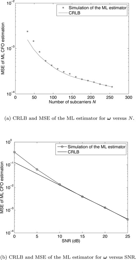
Figure 10.2:  Asymptotic property of the ML estimator.