Chapter 16  Majorization Theory and Applications

Jiaheng Wang^‡ and Daniel Palomar^#

‡ KTH Royal Institute of Technology, Stockholm, Sweden

# Hong Kong University of Science and Technology, Hong Kong

In this chapter we introduce a useful mathematical tool, namely Majorization Theory, and illustrate its applications in a variety of scenarios in signal processing and communication systems. Majorization is a partial ordering and precisely defines the vague notion that the components of a vector are “less spread out” or “more nearly equal” than the components of another vector. Functions that preserve the ordering of majorization are said to be Schur-convex or Schur-concave. Many problems arising in signal processing and communications involve comparing vector-valued strategies or solving optimization problems with vector- or matrix-valued variables. Majorization theory is a key tool that allows us to solve or simplify these problems.

The goal of this chapter is to introduce the basic concepts and results on majorization that serve mostly the problems in signal processing and communications, but by no means to enclose the vast literature on majorization theory. A complete and superb reference on majorization theory is the book by Marshall and Olkin [1]. The building blocks of majorization can be found in [2], and [3] also contains significant material on majorization. Other textbooks on matrix and multivariate analysis, e.g., [4] and [5], may also include a part on majorization. Recent applications of majorization theory to signal processing and communication problems can be found in two good tutorials [6] and [7].

The chapter contains two parts. The first part is devoted to building the framework of majorization theory. The second part focuses on applying the concepts and results introduced in the first part to several problems arising in signal processing and communication systems.

16.1    Majorization Theory

16.1.1    Basic Concepts

To explain the concept of majorization, let us first define the following notations for increasing and decreasing orders of a vector.

Definition 16.1.1. For any vector x ∈ ℝⁿ, let

$x_{\left[1\right]}\ge \cdots \ge x_{\left[n\right]}$

denote its components in decreasing order, and let

$x_{\left(1\right)}\le \cdots \le x_{\left(n\right)}$

denote its components in increasing order.

Majorization¹ defines a partial ordering between two vectors, say x and y, and precisely describes the concept that the components of x are “less spread out” or “more nearly equal” than the components of y.

Definition 16.1.2. (Majorization [1, 1.A.1]) For any two vectors x, y ∈ ℝⁿ, we say x is majorized by y (or y majorizes x), denoted by x ≺ y (or y ≻ x), if

$\begin{array}{cccc}{\displaystyle \sum _{i=1}^k{x}_{\left[i\right]}}& \le & {\displaystyle \sum _{i=1}^k{y}_{\left[i\right]},}& 1\le k<n\\ {\displaystyle \sum _{i=1}^n{x}_{\left[i\right]}}& =& {\displaystyle \sum _{i=1}^n{y}_{\left[i\right]}.}& \end{array}$

Alternatively, the previous conditions can be rewritten as

$\begin{array}{cccc}{\displaystyle \sum _{i=1}^k{x}_{\left(i\right)}}& \ge & {\displaystyle \sum _{i=1}^k{y}_{\left(i\right)},}& 1\le k<n\\ {\displaystyle \sum _{i=1}^n{x}_{\left(i\right)}}& =& {\displaystyle \sum _{i=1}^n{y}_{\left(i\right)}.}& \end{array}$

There are several equivalent characterizations of the majorization relation x ≺ y in addition to the conditions given in Definition 16.1.2. One alternative definition of majorization given in [2] is that x ≺ y if

${\displaystyle \sum _{i=1}^n\varphi \left(x_i\right)}\le {\displaystyle \sum _{i=1}^n\varphi \left(y_i\right)}$

(16.1)

for all continuous convex functions ϕ. Another interesting characterization of x ≺ y, also from [2], is that x = Py for some doubly stochastic matrix² P. In fact, the latter characterization implies that the set of vectors x that satisfy x ≺ y is the convex hull spanned by the n! points formed from the permutations of the elements of y.³ Yet another interesting definition of y ≻ x is given in the form of waterfilling as

${\displaystyle \sum _{i=1}^n{\left(x_i-a\right)}^{+}}\le {\displaystyle \sum _{i=1}^n{\left(y_i-a\right)}^{+}}$

(16.2)

for any a ∈ ℝ and ${\displaystyle {\sum }_{i=1}^n{x}_i={\displaystyle {\sum }_{i=1}^n{y}_{{}_i}}}$, where (u)⁺ ≜ max (u, 0). The interested reader is referred to [1, Ch. 4] for more alternative characterizations.

Observe that the original order of the elements of x and y plays no role in the definition of majorization. In other words, x ≺ Пx for all permutation matrices Π.

Example 16.1.1. The following are simple examples of majorization:

$\begin{array}{l}\left(\frac{1}{n},\frac{1}{n},\dots ,\frac{1}{n}\right)\prec \left(\frac{1}{n-1},\frac{1}{n-1},\dots ,\frac{1}{n-1},0\right)\\ \prec \cdots \prec \left(\frac{1}{2},\frac{1}{2},0,\dots ,0\right)\prec \left(1,0,\dots ,0\right).\end{array}$

More generally

$\left(\frac{1}{n},\frac{1}{n},\dots ,\frac{1}{n}\right)\prec \left(x_1,x_2,\dots ,x_n\right)\prec \left(1,0,\dots ,0\right)$

whenever x_i ≥ 0 and ${\displaystyle {\sum }_{i=1}^n{x}_i=1.}$

□

It is worth pointing out that majorization provides only a partial ordering, meaning that there exist vectors that cannot be compared within the concept of majorization. For example, given x = (0.6, 0.2,0.2) and y = (0.5, 0.4, 0.1), we have neither x ≺ y nor x ≻ y.

To extend Definition 16.1.2, which is only applicable to vectors with the same sum, the following definition provides two partial orderings between two vectors with different sums.

Definition 16.1.3. (Weak majorization [1, 1.A.2]) For any two vectors x, y ∈ ℝⁿ, we say x is weakly submajorized by y (or y submajorizes x), denoted by x ≺_w y (or y ≻_wx), if

${\displaystyle \sum _{i=1}^k{x}_{\left[i\right]}}\le {\displaystyle \sum _{i=1}^k{y}_{\left[i\right]}},1\le k\le n.$

We say x is weakly supermajorized by y (or y supermajorizes x), denoted by x ≺^w y (or y ≻ ^wx), if

${\displaystyle \sum _{i=1}^k{x}_{\left(i\right)}}\le {\displaystyle \sum _{i=1}^k{y}_{\left(i\right)}},1\le k\le n.$

In either case, we say x is weakly majorized by y (or y weakly majorizes x).

For nonnegative vectors, weak majorization can be alternatively characterized in terms of linear transformation by doubly substochastic and superstochastic matrices (see [1, Ch. 2]). Note that x ≺ y implies x ≺_w y and x ≺^w y, but the inverse does not hold. In other words, majorization is a more restrictive definition than weak majorization. A useful connection between majorization and weak majorization is given as follows.

Lemma 16.1.1. ([1, 5.A.9, 5.A.9.a]) If x ≺_w y, then there exist vectors u and v such that

$x\le u\mathrm{and}u\prec y,v\le y\mathrm{and}x\prec v.$

If x ≺^w y, then there exist vectors u and v such that

$x\ge u\mathrm{and}u\prec y,u\ge y\mathrm{and}x\prec v.$

The notation x ≤ u means the componentwise ordering x_i ≤ u_i, i = 1,…, n, for all entries of vectors x, u.

16.1.2    Schur-Convex/Concave Functions

Functions that are monotonic with respect to the ordering of majorization are called Schur-convex or Schur-concave functions. This class of functions is of particular importance in this chapter, as it turns out that many design objectives in signal processing and communication systems are Schur-convex or Schur-concave functions.

Definition 16.1.4. (Schur-convex/concave functions [1, 3.A.1]) A real-valued function ϕ defined on a set $\mathcal{A}$ ⊆ ℝⁿ is said to be Schur-convex on $\mathcal{A}$ if

$x\prec y\mathrm{on}\mathcal{A}\Rightarrow \varphi \left(x\right)\le \varphi \left(y\right).$

If, in addition, ϕ (x) < ϕ (y) whenever x ≺ y but x is not a permutation of y, then ϕ is said to be strictly Schur-convex on $\mathcal{A}$. Similarly, ϕ is said to be Schur-concave on $\mathcal{A}$ if

$x\prec y\mathrm{on}\mathcal{A}\Rightarrow \varphi \left(x\right)\ge \varphi \left(y\right),$

and ϕ is strictly Schur-concave on $\mathcal{A}$ if strict inequality ϕ (x) > ϕ (y) holds when x is not a permutation of y.

Clearly, if ϕ is Schur-convex on $\mathcal{A}$, then −ϕ is Schur-concave on $\mathcal{A}$, and vice versa.

It is important to remark that the sets of Schur-convex and Schur-concave functions do no form a partition of the set of all functions from $\mathcal{A}$ ⊆ ℝⁿ to ℝ. In fact, neither are the two sets disjoint (i.e., the intersection is not empty), unless we consider strictly Schur-convex/concave functions, nor do they cover the entire set of all functions as illustrated in Figure 16.1.

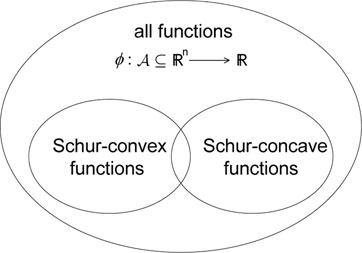
Figure 16.1:  Illustration of the sets of Schur-convex and Schur-concave functions within the set of all functions ϕ : $\mathcal{A}$ ⊆ ℝⁿ → ℝ.

Example 16.1.2. The simplest example of a Schur-convex function, according to the definition, is ϕ (x) = max_k{x_k} = x_[1], which is also strictly Schur-convex.

Example 16.1.3. The function $\varphi \left(x\right)={\displaystyle {\sum }_{i=1}^n{x}_i}$ is both Schur-convex and Schurconcave since ϕ (x) = ϕ (y) for any x ≺ y. However, it is neither strictly Schurconvex nor strictly Schur-concave.

Example 16.1.4. The function ϕ (x) = x₁ + 2x₂ + x₃ is neither Schur-convex nor Schur-concave, as can be seen from the counterexample that for x =(2, 1, 1), y =(2, 2, 0) and z =(4, 0, 0), we have x ≺ y ≺ z but ϕ (x) < ϕ (y) > ϕ (z).

To distinguish Schur-convexity/concavity from common monotonicity, we also define increasing and decreasing functions that will be frequently used later.

Definition 16.1.5. (Increasing/decreasing functions) A function f : ℝⁿ → ℝ is said to be increasing if it is increasing in each argument, i.e.,

$x\le y\Rightarrow f\left(x\right)\le f\left(y\right),$

and to be decreasing if it is decreasing in each argument, i.e.,

$x\le y\Rightarrow f\left(x\right)\ge f\left(y\right).$

Using directly Definition 16.1.4 to check Schur-convexity/concavity of a function may not be easy. In the following, we present some immediate results to determine whether a function is Schur-convex or Schur-concave.

Theorem 16.1.1. ([1, 3.A.3]) Let the function ϕ : $\mathcal{D}$_n → ℝ be continuous on $\mathcal{D}$_n ≜ {x ∈ ℝⁿ : x₁ ≥ ⋯ ≥ x_n} and continuously differentiable on the interior of $\mathcal{D}$_n. Then ϕ is Schur-convex (Schur-concave) on $\mathcal{D}$_n if and only if $\frac{\partial \varphi \left(x\right)}{\partial x_i}$ is decreasing (increasing) in i = 1, …, n.

Theorem 16.1.2. (Schur’s condition [1, 3.A.4]) Let $ℐ$ ⊆ ℝ be an open interval and the function ϕ : ℐⁿ → ℝ be continuously differentiable. Then ϕ is Schur-convex on ℐⁿ if and only if ϕ is symmetric⁴ on ℐⁿ and

$\left(x_i-x_j\right)\left(\frac{\partial \varphi }{\partial x_i}-\frac{\partial \varphi }{\partial x_j}\right)\ge 0,1\le i,j\le n.$

(16.3)

ϕ is Schur-concave on on ℐⁿ if and only if ϕ is symmetric and the inequality (16.3) is reversed.

In fact, to prove Schur-convexity/concavity of a function using Theorem 16.1.1 and Theorem 16.1.2, one can take n = 2 without loss of generality (w.l.o.g.), i.e., check only the two-argument case [1, 3.A.5]. Based on Theorem 16.1.1 and Theorem 16.1.2, it is possible to obtain some sufficient conditions guaranteeing Schur-convexity/concavity of different composite functions.

Proposition 16.1.1. (Monotonic composition [1, 3.B.1]) Consider the composite function ϕ(x) = f (g₁ (x) ,…,g_k (x)), where f is a real-valued function defined on ℝ^k. Then, it follows that

•  f is increasing and g_i is Schur-convex ⇒ ϕ is Schur-convex;

•  f is decreasing and g_i is Schur-convex ⇒ ϕ is Schur-concave;

•  f is increasing and g_i is Schur-concave ⇒ ϕ is Schur-concave;

•  f is decreasing and g_i is Schur-concave ⇒ ϕ is Schur-convex.

Proposition 16.1.2. (Convex⁵ composition [1, 3.B.2]) Consider the composite function ϕ(x) = f (g(x₁),…,g(x_n)), where f is a real-valued function defined on ℝⁿ. Then, it follows that

•  f is increasing Schur-convex and g convex ⇒ ϕ is Schur-convex;

•  f is decreasing Schur-convex and g concave ⇒ ϕ is Schur-convex.

For some special forms of functions, there exist simple conditions to check whether they are Schur-convex or Schur-concave.

Proposition 16.1.3. (Symmetric convex functions [1, 3.C.2]) If ϕ is symmetric and convex (concave), then ϕ is Schur-convex (Schur-concave).

Corollary 16.1.1. ([1, 3.C.1]) Let $\varphi \left(x\right)={\displaystyle {\sum }_{i=1}^{n}g\left(x_i\right)}$, where g is convex (concave). Then ϕ is Schur-convex (Schur-concave).

Proposition 16.1.3 can be generalized to the case of quasi-convex functions.⁶

Proposition 16.1.4. (Symmetric quasi-convex functions [1, 3.C.3]) If ϕ is symmetric and quasi-convex, then ϕ is Schur-convex.

Schur-convexity/concavity can also be extended to weak majorization through the following fact.

Theorem 16.1.3. ( [1, 3.A.8]) A real-valued function ϕ defined on a set $\mathcal{A}$ ⊆ ℝⁿ satisfies

$x{\prec }_{w}y\mathrm{on}\mathcal{A}\Rightarrow \varphi \left(x\right)\le \varphi \left(y\right)$

if and only if ϕ is increasing and Schur-convex on $\mathcal{A}$. Similarly, ϕ satisfies

$x{\prec }^{w}y\mathrm{on}\mathcal{A}\Rightarrow \varphi \left(x\right)\le \varphi \left(y\right)$

if and only if ϕ is decreasing and Schur-convex on $\mathcal{A}$.

By using the above results, we are now able to find various Schurconvex/concave functions. Several such examples are provided in the following, while the interested reader can find more Schur-convex/concave functions in [1].

Example 16.1.5. Consider the l_p norm |x|_p = (Σ_i |x_i|^p)^1/p, which is symmetric and convex when p ≥ 1. Thus, from Proposition 16.1.3, |x|_p is Schur-convex for p ≥ 1.

Example 16.1.6. Suppose that x_i > 0. Since x^a is convex when a ≥ 1 and a ≤ 0 and concave when 0 ≤ a < 1, from Corollary 16.1.1, $\varphi \left(x\right)={\displaystyle {\sum }_i{x}_i^a}$ is Schur-convex for a ≥ 1 and a ≤ 0, and Schur-concave for 0 ≤ a < 1. Similarly, ϕ(x) = ∑_i log x_i and ϕ(x) = −∑_i x_i log x_i are both Schur-concave, since log x and −x log x are concave.

Example 16.1.7. Consider $\varphi :{ℝ}_{+}^2\to ℝ$ with ϕ(x) = −x₁x₂, which is symmetric and quasi-convex. Thus, from Proposition 16.1.4, it is Schur-convex.

16.1.3    Relation to Matrix Theory

There are many interesting results that connect majorization theory to matrix theory, among which a crucial finding by Schur is that the diagonal elements of a Hermitian matrix are majorized by its eigenvalues. This fact has been frequently used to simplify optimization problems with matrix-valued variables.

Theorem 16.1.4. (Schur’s inequality [1, 9.B.1]) Let A be a Hermitian matrix with diagonal elements denoted by the vector d and eigenvalues denoted by the vector λ. Then λ ≻ d.

Theorem 16.1.4 provides an “upper bound” on the diagonal elements of a Hermitian matrix in terms of the majorization ordering. From Exercise 16.1.1, a natural “lower bound” of a vector x ∈ ℝⁿ would be 1 ≺ x, where 1 ∈ ℝⁿ denote the vector with equal elements given by $1_i\triangleq {\displaystyle {\sum }_{j=1}^n{x}_j/n}$. Therefore, for any Hermitian matrix we have

$1\prec d\prec \text{λ}$

(16.4)

which is formally described in the following corollary.

Corollary 16.1.2. Let A be a Hermitian matrix and U a unitary matrix. Then

$1\left(A\right)\prec d\left(U^{†}AU\right)\prec \text{λ}\left(A\right)$

where 1 (A) denotes the vector of equal elements whose sum equal to tr (A), d (A) is the vector of the diagonal elements of A, and λ (A) is the vector of the eigenvalues of A.

Proof: It follows directly from (16.44), as well as the fact that 1 (U^†AU) = 1 (A) and λ (U^†AU) = λ (A).

□

Corollary 16.1.2 “bounds” the diagonal elements of U^†AU for any unitary matrix U. However, it does not specify what can be achieved. The following result will be instrumental for that purpose.

Theorem 16.1.5. ( [1, 9.B.2]) For any two vectors x, y ∈ ℝⁿ satisfying x ≺ y, there exists a real symmetric (and therefore Hermitian) matrix with diagonal elements given by x and eigenvalues given by y.

Corollary 16.1.3. For any vector λ ∈ ℝⁿ, there exists a real symmetric (and therefore Hermitian) matrix with equal diagonal elements and eigenvalues given by λ.

Corollary 16.1.4. Let A be a Hermitian matrix and x ∈ ℝⁿ be a vector satisfying x ≺ λ (A). Then, there exists a unitary matrix U such that

$d\left(U^{†}AU\right)=x.$

Proof: The proofs of Corollary 16.1.3 and Corollary 16.1.4 are straightforward from Corollary 16.1.2 and Theorem 16.1.5.

□

Theorem 16.1.5 is the converse of Theorem 16.1.4 (in fact it is stronger than the converse since it guarantees the existence of a real symmetric matrix instead of just a Hermitian matrix). Now, we can provide the converse of Corollary 16.1.2.

Corollary 16.1.5. Let A be a Hermitian matrix. There exists a unitary matrix U such that

$d\left(U^{†}AU\right)=1\left(A\right),$

and also another unitary matrix U such that

$d\left(U^{†}AU\right)=\text{λ}\left(A\right).$

We now turn to the important algorithmic aspect of majorization theory which is necessary, for example, to compute a matrix with given diagonal elements and eigenvalues. The following definition is instrumental in the derivation of transformations that relate vectors that satisfy the majorization relation.

Definition 16.1.6. (T-transform [1, p. 21]) A T-transform is a matrix of the form

$T=\alpha I+\left(1-\alpha \right)\Pi$

(16.5)

for some α ∈ [0, 1] and some n × n permutation matrix Π with n − 2 diagonal entries equal to 1. Let [Π]_ij = [Π]_ji = 1 for some indices i < j, then

$\Pi y={\left[y_1,\dots ,y_{i-1},y_j,y_{i+1},\dots ,y_{j-1},y_i,y_{j+1},\dots ,y_n\right]}^T$

and hence

$\begin{array}{l}Ty=[y_1,\dots ,y_{i-1},\alpha y_i+\left(1-\alpha \right)y_j,y_{i+1},\dots ,\\ {y_{j-1},\alpha y_j+\left(1-\alpha \right)y_i,y_{j+1},\dots ,y_n]}^T.\end{array}$

Lemma 16.1.2. ([1, 2.B.1]) For any two vectors x, y ∈ ℝⁿ satisfying x ≺ y, there exists a sequence of T-transforms T⁽¹⁾,…, T^(K) such that x = T^(K) ⋯ T⁽¹⁾y and K < n.

An algorithm to obtain such a sequence of T-transforms is introduced next.

Algorithm 16.1.1. ( [1, 2.B.1]) Algorithm to obtain a sequence of T-transforms such that x = T^(K) ⋯ T⁽¹⁾y.

Input: Vectors x, y ∈ ℝⁿ satisfying x ≺ y (it is assumed that the components of x and y are in decreasing order and that x ≠ y).

Output: Set of T-transforms T⁽¹⁾,…, T^(K).

0.  Let y⁽⁰⁾ = y and k = 1 be the iteration index.

1.  Find the largest index i such that $y_i^{\left(k-1\right)}>x_i$ and the smallest index j greater than i such that $y_j^{\left(k-1\right)}<x_j$.

2.  Let δ = min $\delta =\min \left(x_j-y_j^{\left(k-1\right)},y_i^{\left(k-1\right)}-x_i\right)$ and $\alpha =1-\delta /\left(y_i^{\left(k-1\right)}-y_j^{\left(k-1\right)}{}_i\right)$.

3.  Use a to compute T^(k) as in (16.5) and let y^(k) = T^(k)y^(k−1).

4.  If y^(k)≠ x, then set k = k + 1 and go to step 1; otherwise, finish.

Recursive algorithms to obtain a matrix with given eigenvalues and diagonal elements are provided in [1, 9.B.2] and [8]. Here, we introduce the practical and simple method proposed in [8] as follows.

Algorithm 16.1.2. ( [8]) Algorithm to obtain a real symmetric matrix A with diagonal values given by x and eigenvalues given by y provided that x ≺ y.

Input: Vectors x, y ∈ ℝⁿ satisfying x ≺ y (it is assumed that the components of x and y are in decreasing order and that x ≠ y).

Output: Matrix A.

1.  Using Algorithm 16.1.1, obtain a sequence of T-transforms such that x = T^(K) ⋯ T⁽¹⁾y.

2.  Define the Givens rotation U^(k) as

${\left[U^{\left(k\right)}\right]}_{ij}=\{\begin{array}{cc}\sqrt{{\left[T^{\left(k\right)}\right]}_{ij},}& fori<j\\ -\sqrt{{\left[T^{\left(k\right)}\right]}_{ij},}& otherwise.\end{array}$

3.  Let A⁽⁰⁾ = diag (y) and A^(k) = U^(k)TA^(k−1)U^(k). The desired matrix is given by A = A^(K). Define the unitary matrix U = U⁽¹⁾ ⋯ U^(K) and the desired matrix is given by A = U^T diag (y) U.

Algorithm 16.1.2 obtains a real symmetric matrix A with given eigenvalues and diagonal elements. For the interesting case in which the diagonal elements must be equal and the desired matrix is allowed to be complex, it is possible to obtain an alternative much simpler solution in closed form as given next.

Lemma 16.1.3. ( [9]) Let U be a unitary matrix satisfying the condition |[U]_ik| = |[U]_il| ∀i, k, l. Then, the matrix A = U^H diag (λ) U has equal diagonal elements (and eigenvalues given by λ). Two examples of U are the unitary DFT matrix and the Hadamard matrix (when the dimensions are appropriate such as a power of two).

Nevertheless, Algorithm 16.1.2 has the nice property that the obtained matrix U is real-valued and can be naturally decomposed (by construction) as the product of a series of rotations. This simple structure plays a key role for practical implementation. Interestingly, an iterative approach to construct a matrix with equal diagonal elements and with a given set of eigenvalues was obtained in [10], based also on a sequence of rotations.

16.1.4    Multiplicative Majorization

Parallel to the concept of majorization introduced in Section 16.1.1, which is often called additive majorization, is the notion of multiplicative majorization (also termed log-majorization) defined as follows.

Definition 16.1.7. The vector $x\in {ℝ}_{+}^n$ is multiplicatively majorized by $y\in {ℝ}_{+}^n$, denoted by x ≺_× y, if

$\begin{array}{cccc}{\displaystyle \prod _{i=1}^k{x}_{\left[i\right]}}& \le & {\displaystyle \prod _{i=1}^k{y}_{\left[i\right]},}& 1\le k<n\\ {\displaystyle \prod _{i=1}^n{x}_{\left[i\right]}}& =& {\displaystyle \prod _{i=1}^n{y}_{\left[i\right]}}.& \end{array}$

To differentiate the two types of majorization, we sometimes use the symbol ≺₊ rather than ≺ to denote (additive) majorization. It is easy to see the relation between additive majorization and multiplicative majorization: x ≺₊ y if and only if exp(x) ≺_× exp(y).⁷

Example 16.1.8. Given $x\in {ℝ}_{+}^n$, let g denote the vector of equal elements given by $g_i\triangleq {\left({\displaystyle {\prod }_{j=1}^n{x}_j}\right)}^{1/n}$, i.e., the geometric mean of x. Then, g ≺_× x.

Similar to the definition of Schur-convex/concave functions, it is also possible to define multiplicatively Schur-convex/concave functions.

Definition 16.1.8. A function ϕ : $\mathcal{A}$ → ℝ is said to be multiplicatively Schurconvex on $\mathcal{A}$ ∈ ℝⁿ if

$x{\prec }_{\times }y\text{on}\mathcal{A}\Rightarrow \varphi \left(x\right)\le \varphi \left(y\right),$

and multiplicatively Schur-concave on $\mathcal{A}$ if

$x{\prec }_{\times }y\text{on}\mathcal{A}\Rightarrow \varphi \left(x\right)\ge \varphi \left(y\right).$

However, considering the correspondence between additive and multiplicative majorization, it may not be necessary to use the notion of multiplicatively Schur-convex/concave functions. Instead, the so-called multiplicatively Schurconvex/concave functions in Definition 16.1.8 can be equivalently referred to as functions such that ϕ ∘ exp is Schur-convex and Schur-concave, respectively, where the composite function is defined as ϕ ∘ exp$\left(x\right)\triangleq \varphi \left(e^{x_1},\dots ,e^{x_n}\right)$.

The following two lemmas relate Schur-convexity/concavity of a function f with that of the composite function ϕ ∘ exp.

Lemma 16.1.4. If ϕ is increasing and Schur-convex, then ϕ ∘ exp is Schur-convex.

Proof: It is an immediate result from Proposition 16.1.2.

Lemma 16.1.5. If the composite function ϕ ∘ exp is Schur-concave on $\mathcal{D}$_n ≜ {x ∈ ℝⁿ : x₁ ≥ ⋯ ≥ x_n}, then ϕ is Schur-concave on $\mathcal{D}$_n if it is increasing.

Proof: It can be easily proved using Theorem 16.1.1.

The following two examples show that the implication in Lemmas 16.1.4 and 16.1.5 does not hold in the opposite direction.

Example 16.1.9. The function $\varphi \left(x\right)={\displaystyle {\prod }_{i=1}^n{x}_i}$ is Schur-concave on $\mathcal{D}$_n since $\frac{\partial \varphi \left(x\right)}{\partial x_i}=\frac{\varphi \left(x\right)}{x_{{}_i}}$ is increasing in i on $\mathcal{D}$_n (see Theorem 16.1.1). However, the composite function ϕ ∘ exp(x) = exp(∑_i x_i) is Schur-convex (and Schur-concave as well).

Example 16.1.10. The function $\varphi \left(x\right)={\displaystyle {\sum }_{i=1}^n{\alpha }_i{x}_i}$ with α₁ ≤ … ≤ α_n is Schurconcave on $\mathcal{D}$_n. The composite function is $\varphi \circ \exp \left(x\right)={\displaystyle {\sum }_{i=1}^n{\alpha }_{{}_i}\exp }\left(x_i\right)$. For α_i ≤ α_i+1, the derivative $\frac{\partial \varphi \circ \exp \left(x\right)}{\partial x_i}={\alpha }_i$ exp(x_i) is not always monotonic in i = 1,… ,n for any x ∈ $\mathcal{D}$_n. Hence according to Theorem 16.1.1, although ϕ is Schur-concave, ϕ ∘ exp is not Schur-concave (neither Schur-convex) on $\mathcal{D}$_n.

In contrast with (additive) majorization that leads to some important relations between eigenvalues and diagonal elements of a Hermitian matrix (see Section 16.1.3), multiplicative majorization also brings some insights to matrix theory but mostly on the relation between singular values and eigenvalues of a matrix. In the following, we introduce one recent result that will be used later.

Theorem 16.1.6. (Generalized triangular decomposition (GTD) [11]) Let H ∈ ℂ^{m × n} be a matrix with rank k and singular values σ₁ ≥ σ₂ ≥ ⋯ ≥ σ_k. There exists an upper triangular matrix R ∈ ℂ^k×k and semi-unitary matrices Q and P such that H = QRP^H if and only if the diagonal elements of R satisfy |r|≺_×σ, where |r| is a vector with the absolute values of r element-wise. Vectors σ and r stand for the singular values of H and diagonal entries of R, respectively.

The GTD is a generic form including many well-known matrix decompositions such as the SVD, the Schur decomposition, and the QR factorization [4]. Theorem 16.1.6 implies that, given |r|≺_×σ, there exists a matrix H with its singular values and eigenvalues being r and σ, respectively. A recursive algorithm to find such a matrix was proposed in [11].

16.1.5    Stochastic Majorization

A comparison of some kind between two random variables X and Y is called stochastic majorization if the comparison reduces to the ordinary majorization x ≺ y in case X and Y are degenerate at x and y, i.e., Pr (X = x) = 1 and Pr (Y = y) = 1. Random vectors to be compared by stochastic majorization often have distributions belonging to the same parametric family, where the parameter space is a subset of ℝⁿ. In this case, random variables X and Y with corresponding distributions F_θ and F_θ′ are ordered by stochastic majorization if and only if the parameters θ and θ′ are ordered by ordinary majorization.

Specifically, let $\mathcal{A}$ ⊆ ℝⁿ and {F_θ : θ ∈ $\mathcal{A}$} be a family of n-dimensional distribution functions indexed by a vector-valued parameter θ. Let

$E\left\{\varphi \left(X\right)\right\}={\displaystyle {\int }_{{ℝ}^n}\varphi \left(x\right)d{F}_{\theta }\left(x\right)}$

(16.6)

denote the expectation of ϕ(X) when X has distribution F_θ, and let

$\mathrm{Pr}\left(\varphi \left(X\right)\le t\right)={\displaystyle {\int }_{\varphi \left(x\right)\le t}d{F}_{\theta }\left(x\right)}$

(16.7)

denote the tail probability that ϕ(X) is less than or equal to t when X has distribution F_θ. We are particularly interested in investigating whether or in what conditions E {ϕ(X)} and Pr(ϕ(X) ≤ t) are Schur-convex/concave in θ.

The following results provide the conditions in which E {ϕ(X)} is Schur-convex in θ for exchangeable random variables.⁸

Proposition 16.1.5. ([1, 11.B.1]) Let X₁,… ,X_n be exchangeable random variables and suppose that Φ : ℝ²ⁿ → ℝ satisfies: (i) Φ(x, θ) is convex in θ for each fixed x; (ii) Φ(Πx, Πθ) = Φ(x, θ) for all permutations Π; (iii) Φ(x, θ) is Borel measurable in x for each fixed θ. Then,

$\psi \left(\text{θ}\right)=E\left\{\Phi \left(X_1,\dots ,X_n,\text{θ}\right)\right\}$

is symmetric and convex (and thus Schur-convex).

Corollary 16.1.6. ([1, 11.B.2, 11.B.3]) Let X₁,…,X_n be exchangeable random variables and ϕ : ℝⁿ → ℝ be symmetric and convex. Then,

$\psi \left(\text{θ}\right)=E\left\{\varphi \left({\text{θ}}_1{X}_1,\dots ,{\text{θ}}_n{X}_n\right)\right\}$

and

$\psi \left(\text{θ}\right)=E\left\{\varphi \left(X_1+{\text{θ}}_1,\dots ,X_n+{\text{θ}}_n\right)\right\}$

are symmetric and convex (and thus Schur-convex).

Corollary 16.1.7. ([1, 11.B.2.c]) Let X₁,…, X_n be exchangeable random variables and g be a continuous convex function. Then,

$\psi \left(\text{θ}\right)=E\left[g\left({\displaystyle \sum _i{\text{θ}}_i{X}_i}\right)\right]$

is symmetric and convex (and thus Schur-convex).

Compared to the expectation form, there are only a limited number of results on the Schur-convexity/concavity of the tail probability P{ϕ(Χ) ≤ t} in terms of θ, which are usually given in some specific form of ϕ or distribution of X. In the following is one important result concerning linear combinations of some random variables.

Theorem 16.1.7. ( [12]) Let θ_i ≥ 0 for all i, and X₁,…, X_n be independent and identically distributed (iid) random variables following a Gamma distribution with the density

$f\left(x\right)=\frac{x^{k-1}\exp \left(-x\right)}{\Gamma \left(k\right)}$

where Γ(k) = (k − 1)!. Suppose that g : ℝ → ℝ is nonnegative and the inverse function g⁻¹ exists. Then,

$P\left\{g\left({\displaystyle \sum _i{\text{θ}}_i{X}_i}\right)\le t\right\}$

is Schur-concave in θ for t ≥ g(2) and Schur-convex in θ for t ≤ g(1).

Corollary 16.1.8. Let θ_i ≥ 0 for all i, and X₁,…, X_n be iid exponential random variables with the density f (x) = exp(− x). Then, P {∑_i θ_iX_i ≤ t} is Schurconcave in θ for t ≥ 2 and Schur-convex in θ for t ≤ 1.

For more examples of stochastic majorization in the form of expectations or tail probabilities, we refer the interested reader to [1] and [7].

16.2    Applications of Majorization Theory

16.2.1    CDMA Sequence Design

The code division multiple access (CDMA) system is an important multiple-access technique in wireless networks. In a CDMA system, all users share the same bandwidth and they are distinguished from each other by their signature sequences or codes. A fundamental problem in CDMA systems is to optimally design signature sequences so that the system performance, such as the sum capacity, is maximized.

Consider the uplink of a single-cell synchronous CDMA system with K users and processing gain N. In the presence of additive white Gaussian noise, the sampled baseband received signal vector in one symbol interval is

$\mathbf{r}={\displaystyle \sum _{i=1}^K{\mathbf{s}}_i\sqrt{p_i}{b}_i+n}$

(16.8)

where, for each user i, p_i is the received power, b_i is the transmitted symbol, and s_i ∈ ℝ^N is the unit-energy signature sequence, i.e., ‖s_i‖ = 1, and n is a zero-mean Gaussian random vector with covariance matrix σ²Ι_Ν, i.e., n ~ $\mathcal{N}$(0, σ²Ι_Ν). Introduce an N × K signature sequence matrix S ≜ [s₁,…, s_K] and let $P^{1/2}\triangleq \text{diag}\left\{\sqrt{p_1},\dots ,\sqrt{p_K}\right\}$ and b ≜ [b₁,…, b_K]^T. Then (16.8) can be compactly expressed as

$r=S{P}^{1/2}b+n.$

(16.9)

There are different criteria to measure the performance of a CDMA system, among which the most commonly used one may be the sum capacity given by [13]

$C_{\mathrm{sum}}=\frac{1}{2}\log \hspace{0.17em}\det \left(I_N+{\sigma }^{-2}SP{S}^T\right).$

(16.10)

In practice, the system performance may also be measured by the total MSE of all users, which, assuming that each uses a LMMSE filter at his receiver, is given by [14]

$\text{MSE }=K-\text{ Tr}\left[SP{S}^T{\left(SP{S}^T-{\sigma }^2{I}_N\right)}^{-1}\right].$

(16.11)

Another important global quantity that measures the total interference in the CDMA system is the total weighted square correlation (TWSC), which is given by [15]

$\mathrm{TWSC}={\displaystyle \sum _{i=1}^K{\displaystyle \sum _{j=1}^K{p}_i{p}_j\left(s_i^T{s}_j\right)=\mathrm{Tr}\left[{\left(SP{S}^T\right)}^2\right].}}$

(16.12)

The goal of the sequence design problem is to optimize the system performance, e.g., maximize C_sum or minimize MSE or TWSC, by properly choosing the signature sequences for all users or, equivalently, by choosing the optimal signature sequence matrix S.

Observe that the aforementioned three performance measures are all determined by the eigenvalues of the matrix SPS^T. To be more exact, denoting the eigenvalues of SPS^T by $\text{λ}\triangleq {\left({\text{λ}}_i\right)}_{i=1}^N$, it follows that

$\begin{array}{l}{C}_{\text{sum}}=\frac{1}{2}{\displaystyle \sum }_{i=1}^N\log \left(1+\frac{{\text{λ}}_i}{{\sigma }^2}\right)\hfill \\ \text{MSE }=K-{\displaystyle \sum }_{i=1}^N\frac{{\text{λ}}_i}{{\text{λ}}_i+{\sigma }^2}\hfill \\ \text{TWSC }={\displaystyle \sum }_{i=1}^N{\text{λ}}_i^2.\hfill \end{array}$

Now, we can apply majorization theory. Indeed, since log(1 + σ⁻²x) is a concave function, it follows from Corollary 16.1.1 that C_sum is a Schur-concave function with respect to λ. Similarly, given that −x/(x + σ²) and x² are convex functions, both MSE and TWSC are Schur-convex in λ. Therefore, if one can find a signature sequence matrix yielding the Schur-minimal eigenvalues, i.e., one with eigenvalues that are majorized by all other feasible eigenvalues, then the resulting signature sequences will not only maximize C_sum but also minimize MSE and TWSC at the same time.

To find the optimal signature sequence matrix S, let us first define the set of all feasible S

$\mathcal{S}\triangleq \left\{S\in {ℝ}^{N\times K}:\Vert {\mathrm{s}}_i\Vert =1,i=1,\dots ,K\right\}$

(16.13)

and correspondingly the set of all possible λ

$ℒ\triangleq \left\{\text{λ}\left(SP{S}^T\right):S\in \mathcal{S}\right\}.$

(16.14)

Now the question is how to find a Schur-minimal vector within $\mathcal{L}$, which is, however, not easy to answer given the form of $\mathcal{L}$ in (16.14). To overcome this difficulty, we transform $\mathcal{L}$ to a more convenient equivalent form by utilizing the majorization relation.

Lemma 16.2.1. When K ≤ N, $\mathcal{L}$ is equal to

$ℳ\triangleq \left\{\text{λ}\in {ℝ}^N:\left({\text{λ}}_1,\dots ,{\text{λ}}_K\right)\succ \left(p_1,\dots ,p_K\right),{\text{λ}}_{K+1}=\cdots ={\text{λ}}_N=0\right\}.$

When K > N, $\mathcal{L}$ is equal to

$\mathcal{N}\triangleq \left\{\text{λ}\in {ℝ}^N:\left({\text{λ}}_1,\dots ,{\text{λ}}_N,\underset{K-N}{\underbrace{0,\dots ,0}}\right)\succ \left(p_1,\dots ,p_K\right)\right\}.$

Proof: Consider the case K ≤ N. We first show that if λ ∈ ℒ then λ ∈ ℳ. Since K ≤ N, λ(SPS^T) has at most K non-zero elements, which are denoted by λ_a. Let $P\triangleq {\left(p_i\right)}_{i=1}^k$. Observe that, for S ∈ $\mathcal{S}$, p and λ_a are the diagonal elements and the eigenvalues of the matrix P^1/2S^TSP^1/2, respectively. From Theorem 16.1.4 we have λ_a ≻ p, implying that λ ∈ ℳ.

To see the other direction, let λ ∈ ℳ and thus λ_a ≻ p. According to Theorem 16.1.5, there exists a symmetric matrix Z with eigenvalues λ_a and diagonal elements p. Denote the eigenvalue decomposition (EVD) of Z by $Z=U_z{\text{Λ}}_z{U}_z^T$ and introduce Λ = diag{Λ_z, 0_{(N−K)×(N−K)}} and U = [U_z 0_K×(N−K)]. Then we can choose S = Λ^1/2U^TP^−1/2. It is easy to check that the eigenvalues of SPS^T = Λ are λ, and ‖s_i‖², i = 1,…, K, coincide with the diagonal elements of S^TS = P^−1/2ZP^−1/2 and thus are all ones, so we have λ ∈ $\mathcal{L}$.

The equivalence between $\mathcal{L}$ and $\mathcal{N}$ when K > N can be obtained in a similar way, for which a detailed proof was provided in [8].

When K ≤ N, the Schur-minimal vector in $\mathcal{L}$ (or $\mathcal{M}$), from Lemma 16.2.1, is λ* = (p₁,… ,P_L, 0,…, 0), which can be achieved by choosing arbitrary K orthonormal sequences, i.e., S^TS = I_K.

When K > N, the problem of finding a Schur-minimal vector in $\mathcal{L}$ (or $\mathcal{N}$) is, however, not straightforward. It turns out that in this case the Schur-minimal vector is given in a complicated form based on the following definition.

Definition 16.2.1. (Oversized users [8]) User i is defined to be oversized if

$p_i>\frac{{\displaystyle {\sum }_{i=1}^K{p}_j{1}_{\left\{p_i>p_j\right\}}}}{N-{\displaystyle {\sum }_{j=1}^K{1}_{\left\{p_j>p_i\right\}}}}$

where 1_{·} is the indication function. Intuitively, a user is oversized if his power is large relative to those of the others.

Theorem 16.2.1. ([8]) Assume w.l.o.g. that the users are ordered according to their powers p₁ ≥ ⋯ ≥ p_K, and the first L users are oversized. Then, the Schurminimal vector in $\mathcal{L}$ (or $\mathcal{N}$) is given by

${\text{λ}}^{\ast }=\left(p_1,\dots ,p_L,\frac{{\displaystyle {\sum }_{j=L+1}^K{p}_j}}{N-L},\dots ,\frac{{\displaystyle {\sum }_{j=L+1}^K{p}_j}}{N-L}\right).$

The left question is how to find an S ∈ $\mathcal{S}$ such that the eigenvalues of SPS^T are λ*. Note that the constraint S ∈ $\mathcal{S}$ is equivalent to saying that the diagonal elements of S^TS are all equal to 1. Therefore, given the optimal S, the matrix P^1/2S^TSP^1/2 has the diagonal elements p = (p₁,…,p_K) and the eigenvalues λ_b = (λ*, 0). From Theorem 16.1.5, there exists a K × K symmetric matrix M such that its diagonal elements and eigenvalues are given by p and λ_b, respectively. Denote the (EVD) of M by M = UΛU^T, where Λ = diag {λ*} and U ∈ ℝ^{K × N} contains the N eigenvectors corresponding to λ^*. Then, the optimal signature sequence matrix can be obtained as S = Λ^1/2U^TP^−1/2. It can be verified that the eigenvalues of SPS^T are λ* and S ∈ $\mathcal{S}$.

Finally, to construct the symmetric matrix M with the diagonal elements p and the eigenvalues λ_b (provided p ≺ λ_b), one can exploit Algorithm 16.1.2 introduced in Section 16.1.3. Interestingly, an iterative algorithm was proposed in [14, 15] to generate the optimal signature sequences. This algorithm updates each user’s signature sequence in a sequential way, and was proved to converge to the optimal solution.

16.2.2    Linear MIMO Transceiver Design

MIMO channels, usually arising from using multiple antennas at both ends of a wireless link, have been well recognized as an effective way to improve the capacity and reliability of wireless communications [16]. A low-complexity approach to harvest the benefits of MIMO channels is to exploit linear transceivers, i.e., a linear precoder at the transmitter and a linear equalizer at the receiver. Designing linear transceivers for MIMO channels has a long history, but mostly focused on some specific measure of the global performance. It has recently been found in [9, 17] that the design of linear MIMO transceivers can be unified by majorization theory into a general framework that embraces a wide range of different performance criteria. In the following we briefly introduce this unified framework.

Figure 16.2:  Linear MIMO transceiver consisting of a linear precoder and a linear equalizer.

Consider a communication link with N transmit and M receive antennas. The signal model of such a MIMO channel is

$y=Hx+n$

(16.15)

where x ∈ ℂ^N is the transmitted signal vector, H ∈ ℂ^{M × N} is the channel matrix, y ∈ ℂ^M is the received signal vector, and n ∈ ℂ^M is a zero-mean circularly symmetric complex Gaussian random vector with covariance matrix I,⁹ i.e., n ~ $\mathcal{C}\mathcal{N}$(0, I). In the linear transceiver scheme as illustrated in Figure 16.2, the transmitted signal x results from the linear transformation of a symbol vector s ∈ ℂ^L through a linear precoder F ∈ ℂ^{N × L} and is given by x = Fs. Assume w.l.o.g. that L ≤ min{M, N} and E {ss^H} = I. The total average transmit power is

$P_T=E\left\{{\Vert x\Vert }^2\right\}=\mathrm{Tr}\left(F{F}^H\right).$

(16.16)

At the receiver is a linear equalizer G^H ∈ ℂ^{L × M} used to estimate s from y resulting in ŝ = G^H y. Therefore, the relation between the transmitted symbols and the estimated symbols can be expressed as

$\widehat{s}=G^{H}HFs+G^{H}n.$

(16.17)

An advantage of MIMO channels is the support of simultaneously transmitting multiple data streams, leading to significant capacity improvement.¹⁰ Observe from (16.17) that the estimated symbol at the ith data stream is given by

${\widehat{s}}_i={\mathbf{g}}_i^{H}H{\mathrm{f}}_i{s}_i+{\mathbf{g}}_i^H{\mathrm{n}}_i.$

(16.18)

where f_i and g_i are the ith columns of F and G, respectively, and n_i = ∑_j≠iHf _j s _j + n is the equivalent noise seen by the ith data stream with covariance matrix $R_{n_i}={\displaystyle {\sum }_{j\ne i}H{f}_j{f}_j^H}{H}^H+I$. In practice, the performance of a data stream can be measured by the MSE, signal-to-interference-plus-noise ratio (SINR), or bit error rate (BER), which according to (16.18) are given by

$\begin{array}{l}{\mathrm{MSE}}_i\triangleq E\left\{{\left|{\widehat{s}}_i-s_i\right|}^2\right\}={\left|{\mathbf{g}}_i^{H}H{\mathrm{f}}_i-1\right|}^2+{\mathbf{g}}_i^H{R}_{n_i}{g}_i\\ {\mathrm{SINR}}_i\triangleq \frac{\mathrm{desired}\mathrm{component}}{\mathrm{undesired}\mathrm{component}}=\frac{{\left|{\mathbf{g}}_i^{H}H{\mathrm{f}}_i\right|}^2}{{\mathbf{g}}_i^H{R}_{n_i}{g}_i}\\ {\mathrm{BFR}}_i\triangleq \frac{\#\mathrm{bits}\mathrm{in}\mathrm{error}}{\#\mathrm{transmitted}\mathrm{bits}}\approx {\phi }_i\left({\mathrm{SINR}}_i\right)\end{array}$

where φ_i is a decreasing function relating the BER to the SINR at the ith stream [6, 9]. Any properly designed system should attempt to minimize the MSEs, maximize the SINRs, or minimize the BERs.

Measuring the global performance of a MIMO system with several data streams is tricky as there is an inherent tradeoff among the performance of the different streams. Different applications may require a different balance on the performance of the streams, so there are a variety of criteria in the literature, each leading to a particular design problem (see [6] for a survey). However, in fact, all these particular problems can be unified into one framework using the MSEs as the nominal cost. Specifically, suppose that the system performance is measured by an arbitrary global cost function of the MSEs $f_0\left({\left\{{\mathrm{MSE}}_i\right\}}_{i=1}^L\right)$ that is increasing in each argument.¹¹ The linear transceiver design problem is then formulated as

$\begin{array}{cc}\underset{F,G}{\mathrm{minimize}}& f_0\left(\left\{{\mathrm{MSE}}_i\right\}\right)\\ \mathrm{subject}\mathrm{to}& \mathrm{Tr}\left(F{F}^H\right)\le P\end{array}$

(16.19)

where Tr(FF^H) ≤ P represents the transmit power constraint.

To solve (16.19), we first find the optimal G for a fixed F. It turns out that the optimal equalizer is the LMMSE filter, also termed the Wiener filter [19]

$G^{\star }={\left(HF{F}^H{H}^H+I\right)}^{-1}HF.$

(16.20)

To see this, let us introduce the MSE matrix

$\begin{array}{l}E\left(F,G\right)\triangleq E\left[\left(\widehat{\mathbf{s}}-\mathrm{s}\right){\left(\widehat{\mathbf{s}}-\mathbf{s}\right)}^H\right]\\ =\left(G^{H}HF-I\right)\left(F^H{H}^{H}G-I\right)+G^{H}G\end{array}$

(16.21)

from which the MSE of the ith data stream is given by MSE_i = [E]_ii. It is not difficult to verify that

$E\left(F,G^{\star }\right)={\left(I+F^H{H}^{H}HF\right)}^{-1}\underset{\_}{\prec }E\left(F,G\right)$

(16.22)

for any G, meaning that G* simultaneously minimizes all diagonal elements of E or all MSEs. At the same time, one can verify that ${\mathbf{g}}_i^{*}$, i.e., the ith column of G*, also maximizes SINR_i (or equivalently minimizes BER_i) [6, 9]. Hence, the Wiener filter is optimal in the sense of both minimizing all MSEs and maximizing all SINRs (or minimizing all BERs). Observe that the optimality is regardless of the particular choice of the cost function f₀ in (16.19).

Using the Wiener filter as the equalizer, we can easily obtain

$\begin{array}{l}{\mathrm{MSE}}_i={\left[{\left(I+F^H{H}^{H}HF\right)}^{-1}\right]}_{ii}\\ {\mathrm{SINR}}_i=\frac{1}{{\mathrm{MSE}}_i}-1\\ {\mathrm{BER}}_i={\phi }_i\left({\mathrm{MSE}}_i^{-1}-1\right).\end{array}$

This means that different performance measures based on the MSEs, the SINRs, or the BERs can be uniformly represented by the MSE-based criteria, thus indicating the generality of the problem formulation (16.19).

Now, the transceiver design problem (16.19) reduces to the following precoder design problem:

$\begin{array}{ll}\underset{F}{\mathrm{minimize}}\hfill & f_0\left(\left\{{\left[{\left(I+F^H{H}^{H}HF\right)}^{-1}\right]}_{ii}\right\}\right)\hfill \\ \mathrm{subject}\mathrm{to}\hfill & \mathrm{Tr}\left(F{F}^H\right)\le P.\hfill \end{array}$

(16.23)

Solving such a general problem is very challenging and the solution hinges on majorization theory.

Theorem 16.2.2. ( [6, Theorem 3.13]) Suppose that the cost function f₀ : ℝ^L ↦ ℝ is increasing in each argument. Then, the optimal solution to (16.23) is given by

$F^{\star }=V_h\mathrm{diag}\left(\sqrt{p}\right)\Omega$

where

(i)	Vh ∈ ℂN × L is a semi-unitary matrix with columns equal to the right singular vectors of H corresponding to the L largest singular values in increasing order;
(ii)	$\mathrm{p}\in {ℝ}_{+}^L$ is the solution to the following power allocation problem:12

$\begin{array}{ll}\underset{p,\rho }{\mathrm{minimize}}\hfill & f_0\left({\rho }_1,\dots ,{\rho }_L\right)\hfill \\ \mathrm{subject}\mathrm{to}\hfill & \left(\frac{1}{1+p_1{\gamma }_1},\dots ,\frac{1}{1+p_L{\gamma }_L}\right){\succ }^w\left({\rho }_1,\dots ,{\rho }_L\right)\hfill \\ \hfill & p\ge 0,1^{T}p\le P\hfill \end{array}$

(16.24)

where ${\left\{{\gamma }_i\right\}}_{i=1}^L$ are the L largest eigenvalues of H^HH in increasing order;

(iii)

Ω ∈ ℂL × L is a unitary matrix such that [(I + F*HHHHF*)−1]ii = ρi for all i, which can be computed with Algorithm 16.1.2.

Proof: We start by rewriting (16.23) into the equivalent form

$\begin{array}{ll}\underset{F,\rho }{\mathrm{minimize}}\hfill & f_0\left(\rho \right)\hfill \\ \mathrm{subject}\mathrm{to}\hfill & d\left({\left(I+F^H{H}^{H}HF\right)}^{-1}\right)\le \rho \hfill \\ \hfill & \mathrm{Tr}\left(F{F}^H\right)\le P.\hfill \end{array}$

(16.25)

Note that, given any F, we can always find another F̃ = FΩ^H with a unitary matrix Ω such that F̃^HH^HHF̃ = ΩF^HH^HHFΩ^H is diagonal with diagonal elements in increasing order. The original MSE matrix is given by (I + F^HH^HHF)⁻¹ = Ω^H(I + F̃^HH^HHF̃)⁻¹Ω. Thus we can rewrite (16.25) in terms of F̃ and Ω as

$\begin{array}{ll}\underset{\tilde{F},\Omega ,\rho }{\mathrm{minimize}}\hfill & f_0\left(\rho \right)\hfill \\ \mathrm{subject}\mathrm{to}\hfill & {\tilde{F}}^H{H}^{H}H\tilde{F}\mathrm{diagonal}\hfill \\ \hfill & d\left({\Omega }^H{\left(I+{\tilde{F}}^H{H}^{H}H\tilde{F}\right)}^{-1}\Omega \right)\le \rho \hfill \\ \hfill & \mathrm{Tr}\left(\tilde{F}{\tilde{F}}^H\right)\le P.\hfill \end{array}$

(16.26)

It follows from Lemma 16.1.1 and Corollary 16.1.2 that, for a given F̃, we can always find a feasible Ω if and only if

$\text{λ}\left({\left(I+{\tilde{F}}^H{H}^{H}H\tilde{F}\right)}^{-1}\right){\succ }^w\rho .$

Therefore, using the diagonal property of F̃^HH^HHF̃, (16.26) is equivalent to

$\begin{array}{ll}\underset{\tilde{F},\rho }{\mathrm{minimize}}\hfill & f_0\left(\rho \right)\hfill \\ \mathrm{subject}\mathrm{to}\hfill & {\tilde{F}}^H{H}^{H}H\tilde{F}\mathrm{diagonal}\hfill \\ \hfill & d\left({\left(I+{\tilde{F}}^H{H}^{H}H\tilde{F}\right)}^{-1}\right){\succ }^w\rho \hfill \\ \hfill & \mathrm{Tr}\left(\tilde{F}{\tilde{F}}^H\right)\le P.\hfill \end{array}$

(16.27)

Given that F̃^HH^HHF̃ is diagonal with diagonal elements in increasing order, we can invoke [9, Lemma 12] or [6, Lemma 3.16] to conclude that the optimal F̃ can be written as $\tilde{F}=V_h\mathrm{diag}\left(\sqrt{p}\right)$, implying that $F^{*}=V_h\mathrm{diag}\left(\sqrt{p}\right)\Omega$. Now, by using the weak supermajorization relation as well as the structure $\tilde{F}=V_h\mathrm{diag}\left(\sqrt{p}\right)$, (16.27) can be expressed as (16.24).

If, in addition, f₀ is minimized when the arguments are sorted in decreasing order,¹³ then (16.24) can be explicitly written as

$\begin{array}{ll}\underset{p,\rho }{\mathrm{minimize}}\hfill & f_0\left({\rho }_1,\dots ,{\rho }_L\right)\hfill \\ \mathrm{subject}\mathrm{to}\hfill & {\displaystyle {\sum }_{j=i}^L\frac{1}{1+p_i{\gamma }_i}}\le {\displaystyle {\sum }_{j=i}^L{\rho }_j,}1\le i\le L\hfill \\ \hfill & {\rho }_i\ge {\rho }_{i+1},1\le i\le L-1\hfill \\ \hfill & p\ge 0,1^{T}p\le P\hfill \end{array}$

(16.28)

which is a convex problem if f₀ is a convex function, and thus can be efficiently solved in polynomial time [20]. In fact, the optimal precoder can be further simplified or even obtained in closed form, when the objective f₀ falls into the class of Schur-convex/concave functions.

Corollary 16.2.1. ([9, Theorem 1]) Suppose that the cost function f₀ : ℝ^L ↦ ℝ is increasing in each argument.

(i)  If f₀ is Schur-concave, then the optimal solution to (16.23) is given by

$F^{\star }=V_h\mathrm{diag}\left(\sqrt{p}\right)$

where p is the solution to the following power allocation problem:

$\begin{array}{cc}\underset{p}{\mathrm{minimize}}& f_0\left({\left\{{\left(1+p_i{\gamma }_i\right)}^{-1}\right\}}_{i=1}^L\right)\\ \mathrm{subject}\mathrm{to}& p\ge 0,1^{T}p\le P.\end{array}$

(ii) If f₀ is Schur-convex, then the optimal solution to (16.23) is given by

$F^{\star }=V_h\mathrm{diag}\left(\sqrt{p}\right)\Omega$

where the power allocation p is given by

$p_i={\left(\mu {\gamma }_i^{-1/2}-{\gamma }_i^{-1}\right)}^{+},1\le i\le L$

with μ chosen to satisfy 1^Tp = P, and Ω is a unitary matrix such that (I + F*^H H^H HF*)⁻¹ has equal diagonal elements. Ω can be any unitary matrix satisfying |[Ω]_ik| = |[Ω]_il|, ∀i, k, l, such as the unitary DFT matrix or the unitary Hadamard matrix (see Lemma 16.1.3).

Although Schur-convex/concave functions do not form a partition of all L- dimensional functions, they do cover most of the frequently used global performance measures. An extensive account of Schur-convexity/concavity of common performance measures was provided in [6] and [9] (see also Exercise 16.4.3). For Schur-concave functions, a nice property is that the MIMO channel is fully diagonalized by the optimal transceiver, whereas for Schur-convex functions, the channel is diagonalized subject to a specific rotation Ω on the transmit symbols.

16.2.3    Nonlinear MIMO Transceiver Design

In this section, we introduce another paradigm of MIMO transceivers, consisting of a linear precoder and a nonlinear decision feedback equalizer (DFE). The DFE differs from the linear equalizer in that the DFE exploits the finite alphabet property of digital signals and recovers signals successively. Thus, the nonlinear decision feedback (DF) MIMO transceivers usually enjoy superior performance than the linear transceivers. Using majorization theory, the DF MIMO transceiver designs can also be unified, mainly based on the recent results in [11, 21, 22], into a general framework covering diverse design criteria, as was derived independently in [6, 23, 24]. Different from the linear transceiver designs that are based on additive majorization, the DF transceiver designs rely mainly on multiplicative majorization (see Section 16.1.4).

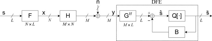
Figure 16.3:  Nonlinear MIMO transceiver consisting of a linear precoder and a decision feedback equalizer (DFE).

Considering the MIMO channel in (16.15), we use a linear precoder F ∈ ℂ^{N × L} at the transmitter to generate the transmitted signal x = Fs from a symbol vector s satisfying E {ss^H} = I. For simplicity, we assume that L ≤ rank(H). The receiver exploits, instead of a linear equalizer, a DFE that detects the symbols successively with the Lth symbol (s_L) detected first and the first symbol (s₁) detected last. As shown in Figure 16.3, a DFE consists of two components: a feed-forward filter G^H ∈ ℂ^{L × M} applied to the received signal y, and a feedback filter B ∈ ℂ^{L × L} that is a strictly upper triangular matrix and feeds back the previously detected symbols. The block Q[·] represents the mapping from the “analog” estimated ŝ_i to the closest “digital” point in the signal constellation. Assuming no error propagation,¹⁴ the “analog” estimated ŝ_i can be written as

${\widehat{s}}_i=g_i^{H}y-{\displaystyle \sum _{j=i+1}^L{b}_{ij}{x}_j,}1\le i\le L$

(16.29)

where g_i is the ith column of G and b_ij = [B]_ij. Compactly, the estimated symbol vector can be written as

$\widehat{s}=G^{H}y-Bs=\left(G^{H}HF-B\right)\mathrm{s}+G^{H}n.$

(16.30)

Let f_i be the ith column of F. The performance of the ith data stream can be measured by the MSE or the SINR as

$\begin{array}{l}{\mathrm{MSE}}_i\triangleq E\left\{{\left|{\widehat{s}}_i-s_i\right|}^2\right\}\\ ={\left|{\mathbf{g}}_i^{H}H{f}_i-1\right|}^2+{\displaystyle \sum _{j=i+1}^L{\left|{\mathbf{g}}_i^{H}H{f}_j-b_{ij}\right|}^2}+{\displaystyle \sum _{j=1}^{i-1}{\left|{\mathbf{g}}_i^{H}H{f}_j\right|}^2+{\Vert g_i\Vert }^2}\\ {\mathrm{SINR}}_i\triangleq \frac{\mathrm{desired}\mathrm{component}}{\mathrm{undesired}\mathrm{component}}\\ =\frac{{\left|{\mathbf{g}}_i^{H}H{f}_i\right|}^2}{{\displaystyle {\sum }_{j=i+1}^L{\left|{\mathbf{g}}_i^{H}H{f}_j-b_{ij}\right|}^2}+{\displaystyle {\sum }_{j=1}^{i-1}{\left|{\mathbf{g}}_i^{H}H{f}_j\right|}^2+{\Vert g_i\Vert }^2}}.\end{array}$

Alternatively, the performance can also be measured by BER_i ≈ φ_i(SINR_i) with a decreasing function φ_i. Similar to the linear transceiver case, we consider that the system performance is measured by a global cost function of the MSEs $f_0\left({\left\{\mathrm{MSE}\right\}}_{i=1}^L\right)$ that is increasing in each argument. Then the nonlinear DF MIMO transceiver design is formulated as the following problem:

$\begin{array}{cc}\underset{F,G,B}{\mathrm{minimize}}& f_0\left(\left\{{\mathrm{MSE}}_i\right\}\right)\\ \mathrm{subject}\mathrm{to}& \mathrm{Tr}\left(F{F}^H\right)\le P\end{array}$

(16.31)

where Tr(FF^H) ≤ P denotes the transmit power constraint.

It is easily seen that to minimize MSE_i, the DF coefficients should be $b_{ij}={\mathbf{\text{g}}}_i^{H}H{f}_j$, 1 ≤ i ≤ j ≤ L, or, equivalently,

$B=\mathcal{U}\left(G^{H}HF\right)$

(16.32)

where $\mathcal{u}$(·) stands for keeping the strictly upper triangular entries of the matrix while setting the others zero. To obtain the optimal feed-forward filter, we let W ≜ HF be the effective channel, and denote by W_i ∈ ℂ^{M × i} the submatrix consisting of the first i columns of W and by w_i the ith column of W. Then, with $b_{ij}=g_i^{H}H{f}_j$, the feed-forward filter minimizing MSE_i is given by [6, Sec. 4.3]

${\mathrm{g}}_i={\left(W_i{W}_i^H+I\right)}^{-1}{w}_i,1\le i\le L.$

(16.33)

In fact, there is a more computationally efficient expression of the optimal DFE given as follows.

Lemma 16.2.2. ([25]) Let the QR decomposition of the augmented matrix be

$W_a\triangleq {\left[\begin{array}{c}W\\ I_L\end{array}\right]}_{\left(M+L\right)\times L}=QR$

and partition Q into

$Q=\left[\begin{array}{c}\overline{Q}\\ \underset{\_}{Q}\end{array}\right]$

where Q̄ ∈ ℂ^{M × L} and Q ∈ ℂ^{L × L}. The optimal feed-forward and feedback matrices that minimize the $\mathrm{MS}\overline{\text{E}}\text{s}$ are

$G^{\star }=\overline{Q}{D}_R^{-1}\mathrm{and}{B}^{\star }=D_R^{-1}R-I$

(16.34)

where D_R is a diagonal matrix with the same diagonal elements as R. The resulting MSE matrix is diagonal:

$E\triangleq E\left[\left(\widehat{\mathbf{s}}-\mathbf{s}\right){\left(\widehat{\mathbf{s}}-\mathbf{s}\right)}^H\right]=D_R^{-2}$

By using the optimal DFE in (16.34), the MSE and the SINR at the ith data stream are related by

${\mathrm{SINR}}_i=\frac{1}{{\mathrm{MSE}}_i}-1$

which is the same as in the linear equalizer case. Therefore, we can focus w.l.o.g. on the MSE-based performance measures, which, according to Lemma 16.2.2, depend on the diagonal elements of R. The optimal precoder is then given by the solution to the following problem:

$\begin{array}{ll}\underset{F}{\mathrm{minimize}}\hfill & f_0\left(\left\{{\left[R\right]}_{ii}^{-2}\right\}\right)\hfill \\ \mathrm{subject}\mathrm{to}\hfill & \left[\begin{array}{c}HF\\ I_L\end{array}\right]=QR\hfill \\ \hfill & \mathrm{Tr}\left(F{F}^H\right)\le P.\hfill \end{array}$

(16.35)

This complicated optimization can be simplified by using multiplicative majorization.

Theorem 16.2.3. ( [6, Theorem 4.3]) Suppose that the cost function f₀ : ℝ^L ↦ ℝ is increasing in each argument. Then, the optimal solution to (16.35) is given by

$F^{\star }=V_h\mathrm{diag}\left(\sqrt{p}\right)\Omega$

where

  (i)  V_h ∈ ℂ^{N × L} is a semi-unitary matrix with columns equal to the right singular vectors of matrix H corresponding to the L largest singular values in increasing order;

 (ii)  $p\in {ℝ}_{+}^L$ is the solution to the following power allocation problem:

$\begin{array}{ll}\underset{p,r}{\mathrm{minimize}}\hfill & f_0\left(r_1^{-2},\dots ,r_L^{-2}\right)\hfill \\ \mathrm{subject}\mathrm{to}\hfill & \left(r_1^2,\dots ,r_L^2\right){\prec }_{\times }\left(1+p_1{\gamma }_1,\dots ,1+p_L{\gamma }_L\right)\hfill \\ \hfill & p\ge 0,1^{T}p\le P\hfill \end{array}$

(16.36)

where ${\left\{{\gamma }_i\right\}}_{i=1}^L$ are the L largest eigenvalues of H^HH in decreasing order;

(iii)  Ω ∈ ℂ^{L × L} is a unitary matrix such that the matrix R in the QR decomposition

$\left[\begin{array}{c}H{F}^{\star }\\ I_L\end{array}\right]=QR$

has diagonal elements ${\left\{r_i\right\}}_{i=1}^L$. To obtain Ω, it suffices to compute the generalized triangular decomposition (GTD) [11]

$\left[\begin{array}{c}H{V}_h\mathrm{diag}\left(\sqrt{p}\right)\\ I_L\end{array}\right]=Q_{J}R{P}_J^H$

and then set Ω = P_J.

Proof: The proof is involved, so we provide only a sketch of it and refer the interested reader to [6, Appendix 4.C] for the detailed proof.

Denote the diagonal elements of R by ${\left\{r_i\right\}}_{i=1}^L$, and the singular values of the effective channel W and the augmented matrix W_a by ${\left\{{\sigma }_{w,1}\right\}}_{i=1}^L$ and ${\left\{{\sigma }_{w_a,1}\right\}}_{i=1}^L$ in decreasing order, respectively. One can easily see that

${\sigma }_{w_a,i}=\sqrt{1+{\sigma }_{w,i}^2}1\le i\le L.$

Consider the SVD $F=U_f\mathrm{diag}\left(\sqrt{p}\right)\Omega$. By using Theorem 16.1.6 on the GTD, one can prove that there exists an Ω such that W_a = QR if and only if $\left\{r_i^2\right\}{\prec }_{\times }\left\{{\sigma }_{w_a,i}^2\right\}$ [6, Lemma 4.9]. Therefore, the constraint

$\left[\begin{array}{c}HF\\ I_L\end{array}\right]=QR$

can be equivalently replaced by

$\left(r_1^2,\dots ,r_L^2\right){\prec }_{\times }\left({\sigma }_{w_a,1}^2,\dots ,{\sigma }_{w_a,L}^2\right).$

Next, by showing that

${\displaystyle \prod _{i=1}^k{\sigma }_{w_a,i}^2}={\displaystyle \prod _{i=1}^k\left(1+{\sigma }_{w,i}^2\right)}\le {\displaystyle \prod _{i=1}^k\left(1+{\gamma }_i{p}_i\right)},1\le k\le L$

where the equality holds if and only if U_f = V_h, one can conclude that the optimal F occurs when U _f = V_h.

Theorem 16.2.3 shows the solution to the general problem with an arbitrary cost function has a nice structure. In fact, when the composite objective function

$f_0\circ \exp \left(\mathrm{x}\right)\triangleq f_0\left(e^{x_1},\dots ,e^{x_L}\right)$

(16.37)

is either Schur-convex or Schur-concave, the nonlinear DF transceiver design problem admits a simpler or even closed-form solution.

Corollary 16.2.2. ([6, Theorem 4.4]) Suppose that the cost function f₀ : ℝ^L ↦ ℝ is increasing in each argument.

 (i)  if f₀ ∘ exp is Schur-concave, then the optimal solution to (16.35) is given by

$F^{\star }=V_h\mathrm{diag}\left(\sqrt{p}\right)$

where p is the solution to the following power allocation problem:

$\begin{array}{cc}\underset{p}{\mathrm{minimize}}& f_0\left(\left\{\left(1+{\gamma }_i{p}_i\right)\right\}\right)\\ \mathrm{subject}\mathrm{to}& p\ge 0,1^{T}p\le P.\end{array}$

(ii)  if f₀ ∘ exp is Schur-convex, then the optimal solution to (16.35) is given by

$F^{\star }=V_h\mathrm{diag}\left(\sqrt{p}\right)\Omega$

where the power allocation p is given by

$p_i={\left(\mu -{\gamma }_i^{-1}\right)}^{+},1\le i\le L$

with μ chosen to satisfy 1^Tp = P, and Ω is a unitary matrix such that the QR decomposition

$\left[\begin{array}{c}H{F}^{\star }\\ I_L\end{array}\right]=QR$

yields R with equal diagonal elements.

It is interesting to relate the linear and nonlinear DF transceivers by the Schurconvexity/concavity of the cost function. From Lemma 16.1.5, f₀ oexp being Schurconcave implies that f₀ is Schur-concave, but not vice versa. From Lemma 16.1.4, if f₀ is Schur-convex, then f₀ ∘ exp is also Schur-convex, but not vice versa. The examples of the cost function for which f₀ ∘ exp is either Schur-concave or Schurconvex were provided in [6] (see also Exercise 16.4.4 and a recent survey [26]).

16.2.4    Impact of Correlation

A Measure of Correlation

Consider two n-dimensional random vectors x and y following the same family/class of distributions with zero means and covariance matrices R_x and R_y, respectively. One question arising in many practical scenarios is how to compare x and y in terms of the degree of correlation. Majorization provides a natural way to measure correlation of a random vector.

Definition 16.2.2. ([7, Sec. 4.1.2]) Let λ(Α) denote the eigenvalues of a positive semidefinite matrix A. Then, we say x is more correlated than y, or the covariance matrix R_x is more correlated than R_y, if λ(R_x) ≻ λ(R_y).

Note that comparing x and y (or equivalently R_x and R_y ) through the majorization ordering imposes an implicit constraint on R_x and R_y that requires ${\displaystyle {\sum }_{i=1}^n{\text{λ}}_i}\left(R_x\right)={\displaystyle {\sum }_{i=1}^n{\text{λ}}_i\left(R_y\right)}$, or equivalently, Tr(R_x) = Tr(R_y). This requirement is actually quite reasonable. If we consider E{|x_i|²} as the “power” of the ith element of x, then $Tr\left(R_x\right)={\displaystyle {\sum }_{i=1}^{n}E\left\{{\left|x_{{}_i}\right|}^2\right\}}$ is the sum power of all elements of x. Therefore, the comparison is conducted in a fair sense that the sum power of the two vectors is equal. Nevertheless, Definition 16.2.2 can be generalized to the case where Tr(R_x) ≠ Tr(R_y) by using weak majorization.

From Example 16.1.1, the most uncorrelated covariance matrix has equal eigenvalues, whereas the most correlated covariance matrix has only one non-zero eigenvalue. In the next, we demonstrate through several examples how to use majorization theory along with Definition 16.2.2 to analyze the effect of correlation on communication systems.

Colored Noise in CDMA Systems

Consider the uplink of a single-cell synchronous CDMA system with K users and processing gain N similar to the one that has been considered in Section 16.2.1 but with colored noise. More exactly, with the received signal at the base station given by (16.8), the zero-mean noise n is now correlated with the covariance matrix R_n. In this case, the sum capacity of the CDMA system is given by [27]

$C_{\mathrm{sum}}=\frac{1}{2}\log \det \left(I_N+R_n^{-1}SP{S}^T\right)$

(16.38)

where S is the signature sequence matrix and P = diag {p₁,… ,p_K} contains the received power of each user. The maximum sum capacity is obtained as C_opt = max_S∈S C_sum, where $\mathcal{S}$ is defined in (16.13).

Denote the EVD of R_n $R_n=U_n{\text{Λ}}_n{U}_n^H$ with eigenvalues ${\sigma }_1^2,\dots ,{\sigma }_N^2$. Then, C_opt can be characterized as follows.

Lemma 16.2.3. ([27, Lemma 2.2]) The maximum sum capacity of the synchronous CDMA system with colored noise is given by

$C_{\mathrm{opt}}=\underset{\mathrm{S}\in \mathcal{S}}{\max }\frac{1}{2}{\displaystyle \sum _{i=1}^N\log \left(1+\frac{{\text{λ}}_i\left(SP{S}^T\right)}{{\sigma }_i^2}\right).}$

(16.39)

Proposition 16.2.1. C_opt obtained in (16.39) is Schur-convex in σ² ≜ $\left({\sigma }_1^2,\dots ,{\sigma }_N^2\right)$.

Proof: Let $\varphi \left({\sigma }^2\right)=\frac{1}{2}{\displaystyle {\sum }_{i=1}^N\log \left(1+{\text{λ}}_i/{\sigma }_i^2\right)}$. Since g(x_i) = log (1 + λ_i/x_i) is a convex function and $f\left(x\right)=\frac{1}{2}{\displaystyle {\sum }_{i=1}^N{x}_i}$ is increasing and Schur-convex, it follows from Proposition 16.1.2 that $\varphi \left({\sigma }^2\right)=f\left(g\left({\sigma }_1^2\right),\dots ,g\left({\sigma }_N^2\right)\right)$ is Schur-convex. Therefore, given ${\sigma }_a^2\prec {\sigma }_b^2$, we have

$C_{\mathrm{opt}}\left({\sigma }_a^2\right)=\underset{\mathrm{S}\in \mathcal{S}}{\max }\varphi \left({\sigma }_a^2\right)\le \underset{\mathrm{S}\in \mathcal{S}}{\max }\varphi \left({\sigma }_b^2\right)=C_{\mathrm{opt}}\left({\sigma }_b^2\right).$

Proposition 16.2.1 indicates that the more correlated (according to Definition 16.2.2) the noise is, the higher the sum capacity could be. Intuitively, if one of the noise variances, say ${\sigma }_N^2$, is much larger than the rest, the users can avoid using signals in the direction of R_n corresponding to ${\sigma }_N^2$ and benefit from a reduced average noise variance (since the sum of all variances keeps unchanged). Apparently, white noise with equal ${\sigma }_i^2={\sigma }^2$, i = 1,…, N, is one of the worst cases that lead to the minimum C_opt.

Spatial Correlation in MISO Channels

A multiple-input single-output (MISO) channel usually arises in using multiple transmit antennas and a single receive antenna in a wireless link. Consider a block-flat-fading¹⁵ MISO channel with N transmit antennas. The channel model is given by

$y=x^{H}h+n$

(16.40)

where x ∈ ℂ^N is the transmitted signal, y ∈ ℂ is the received signal, the complex Gaussian noise n has zero mean and variance σ², and the channel h ∈ ℂ^N is a circular symmetric Gaussian random vector with zero-mean and covariance matrix R_h, i.e., h ~ $\mathcal{CN}$(0, R_h).

In MISO (as well as MIMO) channels, the transmit strategy is determined by the transmit covariance matrix Q = E {xx^H}. Denote the EVD of Q by $Q=U_q{\text{Λ}}_q{U}_q^H$ with the diagonal matrix Λ_q = diag{p₁,… ,p_N}. Then, the eigenvectors of Q, i.e., the columns of U_q, can be regarded as the transmit directions, and the eigenvalue p_i represents the power allocated to the ith data stream or eigenmode. Assuming that the receiver knows the channel perfectly and the transmitter uses a Gaussian codebook with zero mean and covariance matrix Q, the maximum average mutual information, also termed the ergodic capacity, of the MISO channel is given by [16]

$C=\underset{\mathrm{Q}\in \mathcal{Q}}{\max }E\left[\log \left(1+\gamma h^{H}Qh\right)\right]$

(16.41)

where γ is the signal-to-noise ratio, $\mathcal{Q}\triangleq \left\{Q:Q\ge 0,Tr\left(Q\right)=1\right\}$ represents the normalized transmit power constraint, and the expectation is taken over h.

The ergodic capacity depends on what kind of channel state information at the transmitter (CSIT) is available. In the following, we consider three types of CSIT:

•  No CSIT. Neither h nor its statistics are known by the transmitter, and it is usually assumed that h ~ $\mathcal{CN}$(0, I), i.e., R_h = I (see Section 16.2.5).

•  Perfect CSIT. That is, h is perfectly known by the transmitter.

•  Imperfect CSIT with covariance feedback. In this case, it is assumed that h ~ $\mathcal{CN}$(0, R_h) with R_h known by the transmitter.

Denote the EVD of R_h $R_h=U_h{\text{Λ}}_h{U}_h^H$ with eigenvalues μ₁ ≥ ⋯ ≥ μ_Ν sorted w.l.o.g. in decreasing order, and let w₁,…,w_N be standard exponentially iid random variables. In the case of no CSIT, the optimal transmit covariance matrix is given by $Q=\frac{1}{N}I$ [16], which results in

$C_{\mathrm{no}\mathrm{CSIT}}\left(\mu \right)=E\left[\log \left(1+\frac{\gamma }{N}{\displaystyle \sum _{i=1}^N{\mu }_i{w}_i}\right)\right].$

(16.42)

With perfect CSIT, the optimal Q is given by Q = hh^H/ ‖h‖² [16], leading to

$C_{\mathrm{p}\mathrm{CSIT}}\left(\mu \right)=E\left[\log \left(1+\gamma {\displaystyle \sum _{i=1}^N{\mu }_i{w}_i}\right)\right].$

(16.43)

For imperfect CSIT with covariance feedback (i.e., R_h known), the optimal Q is given in the form $Q=U_h{\text{Λ}}_q{U}_h^H$ [28], so the ergodic capacity is obtained by

$C_{\mathrm{cf}\mathrm{CSIT}}\left(\mu \right)=\underset{p\in }{\max }E\left[\log \left(1+\gamma {\displaystyle \sum _{i=1}^N{p}_i{\mu }_i{w}_i}\right)\right]$

(16.44)

where $\mathcal{P}$ ≜ {p : p ≥ 0, 1^Tp = 1} is the power constraint set. The channel capacities of the three types of CSIT all depend on the eigenvalues of R_h, i.e., μ, which is exactly characterized by the following result.

Theorem 16.2.4. ( [29]) While C_noCIST(μ) and C_pCSIT(μ) are both Schur-concave in μ, C_cfCSIT(μ) is Schur-convex in μ.

Proof: The Schur-concavity of C_noCIST(μ) and C_pCSIT(μ) follows readily from Corollary 16.1.6, since $f\left(x\right)=\log \left(1+a{\displaystyle {\sum }_{i=1}^N{x}_i}\right)$ is a symmetric and concave function for a > 0 and x_i > 0. The proof of the Schur-convexity of C_cfCSIT(μ) is based on Theorem 16.1.2 but quite involved. We refer the interested reader to [29] for more details.

□

Theorem 16.2.4 completely characterizes the impact of correlation on the ergodic capacity of a MISO channel. To see this, assume that Tr(R_h) = N (for a fair comparison under Definition 16.2.2) and the correlation vector μ² majorizes μ¹, i.e., μ¹ ≺ μ². We define the fully correlated vector ψ = (N, 0,…, 0) that majorizes all other vectors, and the least correlated vector χ = (1, 1,…, 1) that is majorized by all other vectors. Then, according to Theorem 16.2.4, the impact of different types of CSIT and different levels of correlation on the MISO capacity is provided in the following inequality chain [29]:

$\begin{array}{llllllll}\hfill & C_{\mathrm{no}\mathrm{CSIT}}\left(\psi \right)\hfill & \le \hfill & C_{\mathrm{no}\mathrm{CSIT}}\left({\mu }^2\right)\hfill & \le \hfill & C_{\mathrm{no}\mathrm{CSIT}}\left({\mu }^1\right)\hfill & \le \hfill & C_{\mathrm{no}\mathrm{CSIT}}\left(\chi \right)\hfill \\ =\hfill & C_{\mathrm{cf}\mathrm{CSIT}}\left(\chi \right)\hfill & \le \hfill & C_{\mathrm{cf}\mathrm{CSIT}}\left({\mu }^1\right)\hfill & \le \hfill & C_{\mathrm{cf}\mathrm{CSIT}}\left({\mu }^2\right)\hfill & \le \hfill & C_{\mathrm{cf}\mathrm{CSIT}}\left(\psi \right)\hfill \\ =\hfill & C_{\mathrm{p}\mathrm{CSIT}}\left(\psi \right)\hfill & \le \hfill & C_{\mathrm{p}\mathrm{CSIT}}\left({\mu }^2\right)\hfill & \le \hfill & C_{\mathrm{p}\mathrm{CSIT}}\left({\mu }^1\right)\hfill & \le \hfill & C_{\mathrm{p}\mathrm{CSIT}}\left(\chi \right).\hfill \end{array}$

(16.45)

Simply speaking, correlation helps in the covariance feedback case, but degrades the channel capacity when there is either perfect or no CSIT. Nevertheless, the more amount of CSIT is available, the better the performance could be.

16.2.5    Robust Design

The performance of MIMO communication systems depends, to a substantial extent, on the channel state information (CSI) available at both ends of the communication link. While CSI at the receiver (CSIR) is usually assumed to be perfect, CSI at the transmitter (CSIT) is often imperfect due to many practical issues. Therefore, when devising MIMO transmit strategies, the imperfectness of CSIT has to be considered, leading to the so-called robust designs. A common philosophy of robust designs is to achieve worst-case robustness, i.e., to guarantee the system performance in the worst channel [30]. In this section, we use majorization theory to prove that the uniform power allocation is the worst-case robust solution for two kinds of imperfect CSIT.

Deterministic Imperfect CSIT

Consider the MIMO channel model in (16.15), where the transmit strategy is given by the transmit covariance matrix Q. Indeed, assuming the transmit signal x is a Gaussian random vector with zero mean and covariance matrix Q, i.e., x ~ $\mathcal{CN}$(0, Q), the mutual information is given by [16]

$\Psi \left(Q,H\right)=\log \det \left(I+HQ{H}^H\right)=\log \det \left(I+Q{H}^{H}H\right).$

(16.46)

If H is perfectly known by the transmitter, i.e., perfect CSIT, the channel capacity can be achieved by maximizing Ψ(Q, H) under the power constraint $Q\in \mathcal{Q}\triangleq \left\{Q:Q\ge 0,Tr\left(Q\right)=P\right\}$.

In practice, however, the accurate channel value is usually not available, but belongs to a known set of possible values, often called an uncertainty region. Since Ψ(Q, H) depends on H through R_H = H^HH, we can conveniently define an uncertainty region $\mathcal{H}$ as

$\mathscr{H}\triangleq \left\{H:R_H\in {ℛ}_H\right\}$

(16.47)

where the set $\mathcal{R}$_H could, for example, contain any kind of spectral (eigenvalue) constraints as

${ℛ}_H\triangleq \left\{R_H:\left\{{\text{λ}}_i\left(R_H\right)\right\}\in {ℒ}_{R_H}\right\}$

(16.48)

where ${ℒ}_{R_H}$ denotes arbitrary eigenvalue constraints. Note that $\mathcal{H}$ defined in (16.47) and (16.48) is an isotropic set in the sense that for each H ∈ $\mathcal{H}$ we have HU ∈ $\mathcal{H}$ for any unitary matrix U.

Following the philosophy of worst-case robustness, the robust transmit strategy is obtained by optimizing Ψ(Q, H) in the worst channel within the uncertainty region $\mathcal{H}$, thus resulting in a maximin problem

$\underset{Q\in \mathcal{Q}}{\max }\underset{H\in \mathscr{H}}{\min }\text{Ψ}\left(Q,H\right).$

(16.49)

The optimal value of this maximin problem is referred to as the compound capacity [31]. In the following, we show that the compound capacity is achieved by the uniform power allocation.

Theorem 16.2.5. ( [32, Theorem 1]) The optimal solution to (16.49) is $Q^{*}=\frac{P}{N}I$ and the optimal value is

$C\left(\mathscr{H}\right)=\underset{H\in \mathscr{H}}{\min }\log \det \left(I+\frac{P}{N}{H}^{H}H\right).$

Proof: Denote the eigenvalues of Q by p₁ ≥ •⋯ ≥ p_N w.l.o.g. in decreasing order. From [31, Lemma 1], the optimal Q depends only on {p_i} and thus the inner minimization of (16.49) is equivalent to

$\underset{\left\{{\text{λ}}_i\left(R_H\right)\right\}\in {ℒ}_{R_H}}{\mathrm{minimize}}{\displaystyle \sum _{i=1}^N\log \left(1+p_i{\text{λ}}_i\left(R_H\right)\right)}$

with λ₁(R_H) ≤ ⋯ ≤ λ_N(R_H) in increasing order. Consider the function $f\left(x\right)={\displaystyle {\sum }_{i=1}^N{g}_i\left(x_i\right)={\displaystyle {\sum }_{i=1}^N\log \left(1+a_i{x}_i\right)}}$ with {a_i} in increasing order. It is easy to verify that g′_i(x) ≤ g′_i+1(y) whenever x ≥ y. Thus, from Theorem 16.1.1, f (x) is a Schurconcave function, whose maximum is achieved by a uniform vector x. Under the power constraint ${\displaystyle {\sum }_{i=1}^N{p}_i=P}$, it follows that

$\underset{\left\{{\text{λ}}_i\left(R_H\right)\right\}\in {ℒ}_{R_H}}{\min }{\displaystyle \sum _{i=1}^N\log \left(1+p_i{\text{λ}}_i\left(R_H\right)\right)}\le \underset{\left\{{\text{λ}}_i\left(R_H\right)\right\}\in {ℒ}_{R_H}}{\min }{\displaystyle \sum _{i=1}^N\log \left(1+\frac{P}{N}{\text{λ}}_i\left(R_H\right)\right)}$

where the equality holds for the uniform power allocation.

□

The optimality of the uniform power allocation is actually not very surprising. Due to the symmetry of the problem, if the transmitter does not uniformly distribute power over the eigenvalues of Q, then the worst channel will align its highest singular value (or eigenvalue of R_H ) to the lowest eigenvalue of Q. Therefore, to avoid such a situation and achieve the best performance in the worst channel, an appropriate way is to use equal power on all eigenvalues of Q, which is formally proved in Theorem 16.2.5.

Stochastic Imperfect CSIT

Tracking the instantaneous channel value may be difficult when the channel varies rapidly. The stochastic imperfect CSIT model assumes that the channel is a random quantity with its statistics such as mean or/and covariance known by the transmitter. Sometimes, even the channel statistics may not be perfectly known. The interests of this model would be on optimizing the average system performance using the channel statistics.

For simplicity, we consider the MISO channel in (16.40), where the channel h is a circular symmetric Gaussian random vector with zero-mean and covariance matrix R_h, i.e., h ~ $\mathcal{CN}$(0, R_h). Mathematically, the channel can be expressed as

$h=R_h^{1/2}z$

(16.50)

where z ~ $\mathcal{CN}$(0, I). Different from the covariance feedback case where R_h is assumed to be known by the transmitter (see Section 16.2.4), here we consider an extreme case where the transmitter does not even know exactly R_h. Instead, we assume that R_h ∈ $\mathcal{R}$_h with

${ℛ}_h\triangleq \left\{R_h:\left\{{\text{λ}}_i\left(R_h\right)\right\}\in {ℒ}_{{\mathrm{R}}_h}\right\}$

(16.51)

where ${ℒ}_{R_h}$ denotes arbitrary constraints on the eigenvalues of R_h. In the case of no information on R_h, we have ${ℒ}_{R_h}={ℝ}_{+}^N$. To combat with the possible bad channels, the robust transmit strategy should take into account the worst channel covariance, thus leading to the following maximin problem

$\underset{Q\in \mathcal{Q}}{\max }\underset{R_h\in {ℛ}_h}{\min }E\left[\log \left(1+h^{H}Qh\right)\right]=E\left[\log \left(1+z^H{R}_h^{1/2}Q{R}_h^{1/2}z\right)\right]$

(16.52)

where $\mathcal{Q}\triangleq \left\{Q:Q\ge 0,\mathrm{Tr}\left(Q\right)=P\right\}$ and z ~ $\mathcal{CN}$(0, I). The following result indicates that the uniform power allocation is again the robust solution.

Theorem 16.2.6. The optimal solution to (16.52) is $Q^{*}=\frac{P}{N}I$ and the optimal value is

$C\left({ℛ}_h\right)\underset{R_h\in {ℛ}_h}{\min }E\left[\log \left(1+\frac{P}{N}{\displaystyle \sum _{i=1}^N{\text{λ}}_i\left(R_h\right)w_i}\right)\right]$

where w₁, … ,W_N are standard exponentially iid random variables.

Proof: Denote the eigenvalues of Q by p₁ ≥ ⋯ ≥ p_N w.l.o.g. in decreasing order. Considering that Q and $\mathcal{R}$_h impose no constraint on the eigenvectors of Q and R_h, respectively, and that Uz has the same distribution as z for any unitary matrix U, the optimal Q should be a diagonal matrix depending on the eigenvalues {p_i} (see, e.g., [28]) and thus (16.52) is equivalent to

$\underset{Q\in \mathcal{Q}}{\max }\underset{R_h\in {ℛ}_h}{\min }E\left[\log \left(1+{\displaystyle \sum _{i=1}^N{p}_i{\text{λ}}_i\left(R_h\right)w_i}\right)\right]$

(16.53)

with w_i = |z_i|², where z_i is the ith element of z.

Given {p_i} in decreasing order, the minimum of the inner minimization of (16.53) must be achieved with {λ_i(R_h)} in increasing order, otherwise a smaller objective value can be obtained by changing the order of {λ_i(R_h)}. Then, following the similar steps in the proof of Theorem 16.2.5, one can show that $E\left\{\log \left(1+{\displaystyle {\sum }_{i=1}^N{p}_i{\text{λ}}_i\left(R_h\right)w_i}\right)\right\}$ is a Schur-concave function with respect to ${\left(p_{{}_i}\right)}_{i=1}^N$. Hence, the maximum of (16.53) is achieved by a uniform power vector that is majorized by all other power vectors under the constraint ${\displaystyle {\sum }_{i=1}^N{p}_i=P}$.

Another interesting problem is to investigate the worst channel correlation for all possible transmit strategies, which is given by the solution to the following minimax problem:

$\underset{R_h\in {ℛ}_h}{\min }\underset{Q\in \mathcal{Q}}{\max }E\left[\log \left(1+h^{H}Qh\right)\right].$

(16.54)

Through the similar steps in the proof of Theorem 16.2.6, one can find that the solution to (16.54) is proportional to an identity matrix, i.e., R_h = αI with α > 0. This provides a robust explanation for the assumption that h ~ $\mathcal{CN}$(0, I) in the case of no CSIT (see Section 16.2.4): R_h = I is the worst correlation among $\mathcal{R}$_h = {R_h : Tr(R_h) = N} [29].

16.3    Conclusions and Further Readings

This chapter introduced majorization as a partial order relationship for real-valued vectors and described its main properties. This chapter also presented applications of majorization theory in proving inequalities and solving various optimization problems in the fields of signal processing and wireless communications. For a more comprehensive treatment of majorization theory and its applications, the readers are directed to Marshall and Olkins book [1]. Applications of majorization theory to signal processing and wireless communications are also described in the tutorials [6] and [7] .

16.4    Exercises

Exercise 16.4.1. Schur-convexity of sums of functions.

a.  Let $\varphi \left(x\right)={\displaystyle {\sum }_{i=1}^n{g}_i\left(x_i\right)}$, where each g_i is differentiable. Show that ϕ is Schur-convex on $\mathcal{D}$_n if and only if

${g^{\prime }}_i\left(a\right)\ge {g^{\prime }}_{i+1}\left(b\right)\mathrm{whenever}a\ge b,i=1,\dots ,n-1.$

b.  Let $\varphi \left(x\right)={\displaystyle {\sum }_{i=1}^n{a}_{i}g\left(x_i\right)}$, where g (x) is decreasing and convex, and 0 ≤ a₁ ≤ ⋯ ≤ a_n. Show that ϕ is Schur-convex on $\mathcal{D}$_n.

Exercise 16.4.2. Schur-convexity of products of functions.

a.  Let g : $\mathcal{I}$ → ℝ₊ be continuous on the interval $\mathcal{I}$ ⊆ ℝ. Show that ϕ(x) = ${\displaystyle {\prod }_{i=1}^{n}g\left(x_i\right)}$ is (strictly) Schur-convex on $\mathcal{I}$ⁿ if and only if log g is (strictly) convex on $\mathcal{I}$.

b.  Show that $\varphi \left(x\right)={\displaystyle {\prod }_{i=1}^n\Gamma \left(x_i\right)}$, where $\Gamma \left(x\right)={\displaystyle {\int }_0^{\infty }{u}^{x-1}{e}^{-u}du}$ denotes the Gamma function, is strictly Schur-convex on ${ℝ}_{++}^n$.

Exercise 16.4.3. Linear MIMO Transceiver.

a.  Prove Corollary 16.2.1, which shows that when the cost function f₀ is either Schur-concave or Schur-convex, the optimal linear MIMO transceiver admits an analytical structure.

b.  Show that the following problem formulations can be rewritten as minimizing a Schur-concave cost function of MSEs:

•  Minimizing $f\left(\left\{{\mathrm{MSE}}_i\right\}\right)={\displaystyle {\sum }_{i=1}^L{\alpha }_i{\mathrm{MSE}}_i}$.¹⁶

•  Minimizing $f\left(\left\{{\mathrm{MSE}}_i\right\}\right)={\displaystyle {\prod }_{i=1}^L{\mathrm{MSE}}_i^{{\alpha }_{{}_i}}}$.

•  Maximizing $f\left(\left\{{\mathrm{SINR}}_i\right\}\right)={\displaystyle {\sum }_{i=1}^L{\alpha }_i{\mathrm{SINR}}_i}$.

•  Maximizing $f\left(\left\{{\mathrm{SINR}}_i\right\}\right)={\displaystyle {\prod }_{i=1}^L{\mathrm{SINR}}_i^{{\alpha }_i}}$.

•  Minimizing $f\left(\left\{{\mathrm{BER}}_i\right\}\right)={\displaystyle {\prod }_{i=1}^L{\mathrm{BER}}_{{}_i}}$.

c.  Show that the following problem formulations can be rewritten as minimizing a Schur-convex cost function of MSEs:

•  Minimizing $f\left(\left\{{\mathrm{MSE}}_i\right\}\right)={\max }_i\left\{{\mathrm{MSE}}_i\right\}$.

•  Maximizing $f\left(\left\{{\mathrm{SINR}}_i\right\}\right)={\left({\displaystyle {\prod }_{i=1}^L{\mathrm{SINR}}_i^{-1}}\right)}^{-1}$.

•  Maximizing $f\left(\left\{{\mathrm{SINR}}_{i_{{}_i}}\right\}\right)={\min }_i\left\{{\mathrm{SINR}}_{{}_i}\right\}$.

•  Minimizing $f\left(\left\{{\mathrm{BER}}_i\right\}\right)={\displaystyle {\sum }_{i=1}^L{\mathrm{BER}}_i}$.

•  Minimizing $f\left(\left\{{\mathrm{BER}}_i\right\}\right)={\max }_i\left\{{\mathrm{BER}}_i\right\}$.

Exercise 16.4.4. Nonlinear MIMO Transceiver.

a.  Prove Corollary 16.2.2, which shows that the optimal nonlinear DF MIMO transceiver can also be analytically characterized if the composite cost function f₀ ∘ exp is either Schur-concave or Schur-convex.

b.  Show that the following problem formulations can be rewritten as minimizing a Schur-concave f₀ ∘ exp of MSEs:

•  Minimizing $f\left(\left\{{\mathrm{MSE}}_i\right\}\right)={\displaystyle {\prod }_{i=1}^L{\mathrm{MSE}}_i^{{\alpha }_i}}$.

•  Maximizing $f\left(\left\{{\mathrm{SINR}}_i\right\}\right)={\displaystyle {\sum }_{i=1}^L{\alpha }_i{\mathrm{SINR}}_i}$.

Show that, in addition to all problem formulations in Exercise 16.4.3.c, the following ones can also be rewritten as minimizing a Schur-convex f₀ ∘ exp of MSEs:

•  Minimizing $f\left(\left\{{\mathrm{MSE}}_i\right\}\right)={\displaystyle {\sum }_{i=1}^L{\mathrm{MSE}}_i}$.

•  Minimizing $f\left(\left\{{\mathrm{MSE}}_i\right\}\right)={\displaystyle {\prod }_{i=1}^L{\mathrm{MSE}}_i}$.

•  Maximizing $f\left(\left\{{\mathrm{SINR}}_i\right\}\right)={\displaystyle {\prod }_{i=1}^L{\mathrm{SINR}}_i}$.

References

[1]   A. W. Marshall and I. Olkin, Inequalities: Theory of Majorization and Its Applications. New York: Academic Press, 1979.

[2]   G. H. Hardy, J. E. Littlewood, and G. Pólya, Inequalities, 2nd ed. London and New York: Cambridge University Press, 1952.

[3]   R. Bhatia, Matrix Analysis. New York: Springer-Verlag, 1997.

[4]   R. A. Horn and C. R. Johnson, Matrix Analysis. New York: Cambridge University Press, 1985.

[5]   T. W. Anderson, An Introduction to Multivariate Statistical Analysis, 3rd ed. Hoboken, NJ: Wiley, 2003.

[6]   D. P. Palomar and Y. Jiang, “MIMO transceiver design via majorization theory,” Foundations and Trends in Communications and Information Theory, vol. 3, no. 4–5, pp. 331–551, 2006.

[7]   E. A. Jorswieck and H. Boche, “Majorization and matrix-monotone funcstions in wireless communications,” Foundations and Trends in Communications and Information Theory, vol. 3, no. 6, pp. 553–701, Jul. 2006.

[8]   P. Viswanath and V. Anantharam, “Optimal sequences and sum capacity of synchronous CDMA systems,” IEEE Trans. Inform. Theory, vol. 45, no. 6, pp. 1984–1993, Sep. 1999.

[9]   D. P. Palomar, J. M. Cioffi, and M. A. Lagunas, “Joint Tx-Rx beamforming design for multicarrier MIMO channels: A unified framework for convex optimization,” IEEE Trans. Signal Process., vol. 51, no. 9, pp. 2381–2401, Sep. 2003.

[10]   C. T. Mullis and R. A. Roberts, “Synthesis of minimum roundoff noise fixed point digital filters,” IEEE Trans. on Circuits and Systems, vol. CAS-23, no. 9, pp. 551–562, Sept. 1976.

[11]   Y. Jiang, W. Hager, and J. Li, “The generalized triangular decomposition,” Mathematics of Computation, Nov. 2006.

[12]   E. A. Jorswieck and H. Boche, “Outage probability in multiple antenna systems,” European Transactions on Telecommunications, vol. 18, no. 3, pp. 217–233, Apr. 2007.

[13]   S. Verdú, Multiuser Detection. New York, NY: Cambridge University Press, 1998.

[14]   S. Ulukus and R. D. Yates, “Iterative construction of optimum signature sequence sets in synchronous CDMA systems,” IEEE Trans. Inform. Theory, vol. 47, no. 5, pp. 1989–1998, Jul. 2001.

[15]   C. Rose, S. Ulukus, and R. D. Yates, “Wireless systems and interference avoidance,” IEEE Trans. Wireless Commun., vol. 1, no. 3, pp. 415–428, Jul. 2002.

[16]   I. E. Telatar, “Capacity of multi-antenna Gaussian channels,” European Trans. Telecommun., vol. 10, no. 6, pp. 585–595, Nov.-Dec. 1999.

[17]   D. P. Palomar, M. A. Lagunas, and J. M. Cioffi, “Optimum linear joint transmit-receive processing for MIMO channels with QoS constraints,” IEEE Trans. Signal Process., vol. 52, no. 5, pp. 1179–1197, May 2004.

[18]   L. Zheng and D. N. C. Tse, “Diversity and multiplexing: A fundamental tradeoff in multiple-antenna channels,” IEEE Trans. Inform. Theory, vol. 49, no. 5, pp. 1073–1096, May 2003.

[19]   S. M. Kay, Fundamentals of Statistical Signal Processing: Estimation Theory. Englewood Cliffs, NJ, USA: Prentice-Hall, 1993.

[20]   S. Boyd and L. Vandenberghe, Convex Optimization. Cambridge, U.K.: Cambridge University Press, 2004.

[21]   Y. Jiang, W. Hager, and J. Li, “The geometric mean decomposition,” Linear Algebra and Its Applications, vol. 396, pp. 373–384, Feb. 2005.

[22]   Y. Jiang, W. Hager, and J. Li, “Tunable channel decomposition for MIMO communications using channel state information,” IEEE Trans. Signal Process., vol. 54, no. 11, pp. 4405–4418, Nov. 2006.

[23]   F. Xu, T. N. Davidson, J. K. Zhang, and K. M. Wong, “Design of block transceivers with decision feedback detection,” IEEE Trans. Signal Process., vol. 54, no. 3, pp. 965–978, Mar. 2006.

[24]   A. A. D’Amico, “Tomlinson-Harashima precoding in MIMO systems: A unified approach to transceiver optimization based on multiplicative schurconvexity,” IEEE Trans. Signal Process., vol. 56, no. 8, pp. 3662–3677, Aug. 2008.

[25]   B. Hassibi, “A fast square-root implementation for BLAST,” in Proc. of Thirty-Fourth Asilomar Conference on Signals, Systems and Computers, Pacific Grove, CA, USA, Nov. 2000.

[26]   P. P. Vaidyanathan, S.-M. Phoong, and Y.-P. Lin, Signal Processing and Optimization for Transceiver Systems. New York, NY: Cambridge University Press, 2010.

[27]   P. Viswanath and V. Anantharam, “Optimal sequences for CDMA under colored noise: A Schur-saddle function property,” IEEE Trans. Inform. Theory, vol. 48, no. 6, pp. 1295–1318, Jun. 2002.

[28]   S. A. Jafar and A. Goldsmith, “Transmitter optimization and optimality of beamforming for multiple antenna systems,” IEEE Trans. Wireless Commun., vol. 3, no. 4, pp. 1165–1175, Jul. 2004.

[29]   E. A. Jorswieck and H. Boche, “Optimal transmission strategies and impact of correlation in multiantenna systems with different types of channel state information,” IEEE Trans. Signal Process., vol. 52, no. 12, pp. 3440–3453, Dec. 2004.

[30]   J. Wang and D. P. Palomar, “Worst-case robust MIMO transmission with imperfect channel knowledge,” IEEE Trans. Signal Process., vol. 57, no. 8, pp. 3086–3100, Aug. 2009.

[31]   A. Lapidoth and P. Narayan, “Reliable communication under channel uncertainty,” IEEE Trans. Inform. Theory, vol. 44, no. 6, pp. 2148–2177, Oct. 1998.

[32]   D. P. Palomar, J. M. Cioffi, and M. A. Lagunas, “Uniform power allocation in MIMO channels: A game-theoretic approach,” IEEE Trans. Inform. Theory, vol. 49, no. 7, pp. 1707–1727, Jul. 2003.

¹The majorization ordering given in Definition 16.1.2 is also called additive majorization, to distinguish it from multiplicative majorization (or log-majorization) introduced in Section 16.1.4.

²A square matrix P is said to be stochastic if either its rows or columns are probability vectors, i.e., if its elements are all nonnegative and either the rows or the columns sums are one. If both the rows and columns are probability vectors, then the matrix is called doubly stochastic. Stochastic matrices can be considered representations of the transition probabilities of a finite Markov chain.

³The permutation matrices are doubly stochastic and, in fact, the convex hull of the permutation matrices coincides with the set of doubly stochastic matrices [1, 2].

⁴A function is said to be symmetric if its arguments can be arbitrarily permuted without changing the function value.

⁵A function f : χ → ℝ is convex if χ is a convex set and for any x,y ∈ χ and 0 ≤ α ≤ 1, f (αx + (1 − α) y) ≤ αf (x) + (1 − α) f (y). f is concave if −f is convex.

⁶A function f : χ → ℝ is quasi-convex if χ is a convex set and for any x,y ∈ χ and 0 ≤ α ≤ 1, f (αx + (1 − α)y) ≤ max{f (x), f (y)}. A convex function is also quasi-convex, but the converse is not true.

⁷Indeed, using the language of group theory, we say that the groups (ℝ, +) and (ℝ₊, ×) are isomorphic since there is a bijection function exp : ℝ → ℝ+ such that exp(x+y) = exp(x) × exp(y) for ∀ x, y ∈ ℝ.

⁸X₁ ,…,X_n are exchangeable random variables if the distribution of Χ_π(1),…, X_π(n) does not depend on the permutation π. In other words, the joint distribution of X₁,…, X_n is invariant under permutations of its arguments. For example, independent and identically distributed random variables are exchangeable.

⁹If the noise is not white, say with covariance matrix R_n, one can always whiten it by y̅ = $R_n^{-1/2}y=\overline{H}x+\overline{n}$, where $\overline{H}=R_n^{-1/2}H$ is the equivalent channel.

¹⁰This kind of improvement is often called the multiplexing gain [18].

¹¹The increasingness of f is a mild and reasonable assumption: if the performance of one stream improves, the global performance should improve too.

¹²≻^w denotes weak supermajorization (see Definition 16.1.3).

¹³In practice, most cost functions are minimized when the arguments are in a specific ordering (if not, one can always use instead the function f̃₀(x) = min_p∈Ƥ f₀(Px), where Ƥ is the set of all permutation matrices) and, hence, the decreasing order can be taken without loss of generality.

¹⁴Error propagation means that if the detection is erroneous, it may cause more errors in the subsequent detections. By using powerful coding techniques, the influence of error propagation can be made negligible.

¹⁵Block flat-fading means that the channel keeps unchanged for a block of T symbols, and then the channel changes to an uncorrelated channel realization.

¹⁶Assume w.l.o.g. that 0 ≤ α₁ ≤ ⋯ ≤ α_L.