7 Probability, Random Variables, and Stochastic Processes

Search in book...
Toggle Font Controls
Create new playlist

Name your new playlist

Playlist description (optional)
Sign In

Email address

Password

Forgot Password?

or

Continue with Facebook

Continue with Google
Sign Up

Full Name

Email address

Confirm Email Address

Password

or

Continue with Facebook

Continue with Google

Dinesh Rajan‡

‡ Southern Methodist University, Dallas, USA

Probability theory essentially provides a framework and tools to quantify and predict the chance of occurrence of an event in the presence of uncertainties. Probability theory also provides a logical way to make decisions in situations where the outcomes are uncertain. Probability theory has widespread applications in a plethora of different fields such as financial modeling, weather prediction, and engineering. The literature on probability theory is rich and extensive. A partial list of excellent references includes [1, 5]. The goal of this chapter is to focus on the basic results and illustrate the theory with several numerical examples. The proofs of the major results are not provided and relegated to the references.

While there are many different philosophical approaches to define and derive probability theory, Kolmogorov’s axiomatic approach is the most widely used. This axiomatic approach begins by defining a small number of precise axioms or postulates and then deriving the rest of the theory from these postulates.

Before formally defining Kolmogorov’s axioms, we first specify the basic framework to understand and study probability theory. Probability is essentially defined in the context of a repeatable random experiment. An experiment consists of a procedure for conducting the experiment and a set of outcomes/observations of the experiment. A model is assigned to the experiment which affects the occurrence of the various outcomes. A sample space, S, is a collection of finest grain, mutually exclusive and collectively exhaustive set of all possible outcomes. Each element ω of the sample space S represents a particular outcome of the experiment. An event E is a collection of outcomes.

Example 7.1.1. A fair coin is tossed three times. The sample space S = {HHH, HHT, HTH, HTT, THH, THT, TTH, TTT}. Event E₁ = {HTT, THT, TTH} is the set of all outcomes with exactly 1 Head in the three coin flips.

□

Example 7.1.2. The angle that the needle makes in a wheel of fortune game is observed. The sample space S = {θ : 0 ≤ 9 < 2π}.

□

Events E_j and E_k are said to be mutually exclusive or disjoint events if there are no outcomes that are common to both events, i.e., E_j ∩ E_k = ϕ.

A collection of events $ℱ$ $ℱ$ defined over a sample space S is called a sigma field if:

• $ℱ$ $ℱ$ includes both the impossible event ϕ and the certain event S.

• For every set A ⊂ $ℱ$ $ℱ$ , it implies that A^c ⊂ $ℱ$ $ℱ$ .

• $ℱ$ $ℱ$ is closed under countable set operations of union and intersection, i.e., A ∩ B ∩ $ℱ$ $ℱ$ and A ∪ B ⊂ $ℱ$ $ℱ$ , ∀A, B ⊂ $ℱ$ $ℱ$ .

Given a sigma Field $ℱ$ $ℱ$ , a probability measure Pr (·) is a mapping from every event A ⊂ $ℱ$ $ℱ$ to a real number Pr (A) called the probability of event A satisfying the following three axioms:

1. Pr (A) ≥ 0.

2. Pr (S) = 1.

3. For a countable collection of mutually exclusive events A₁,A₂,…, Pr (A₁ ∪ A₂ ∪ A₃ ∪ …) = Pr (A₁) + Pr (A₂) + Pr (A₃) + …

A probability space consists of the triplet (S, $ℱ$ $ℱ$ , P).

Example 7.1.3. A fair coin is flipped 1 time. In this case, S = {H,T}. The sigma field $ℱ$ $ℱ$ consists of the sets, {H}, {T}, {ϕ}, {S}. The probability measure maps these sets to the probabilities as follows: Pr (H) = Pr (T) = 0.5, Pr (ϕ) = 0, and Pr (S) = 1.

□

The following simple and intuitive properties of the probability of an event can be readily derived from these axioms:

• The probability of the null set equals 0, i.e., Pr (ϕ) = 0.

• The probability of any event A is no greater than 1, i.e., Pr (A) ≤ 1.

• The sum of the probability of an event and the probability of its complement equals 1, i.e., Pr (A^c) = 1 − Pr (A).

• If A ⊂ B then Pr (A) ≤ Pr (B).

• The probability of the union of events A and B can be expressed in terms of the probability of events A, B and their intersection A ∩ B, i.e.,

$\Pr (A \cup B) = \Pr (A) + \Pr (B) - \Pr (A \cap B) .$ $\Pr (A \cup B) = \Pr (A) + \Pr (B) - \Pr (A \cap B) .$

(7.1)

To prove (7.1), we can express A ∪ B in terms of three mutually exclusive sets A₁ = A ∩ B, A₂ = A − B and A₃ = B − A. Hence, Pr (A ∪ B) = Pr (A₁) + Pr (A₂) + Pr(A₃). Then by applying Axiom 3, we obtain Pr (A) = Pr(A₁) + Pr(A₂) and Pr(B) = Pr (A₁) + Pr(A₃). Property (7.1) readily follows. The other properties stated above can be similarly proved.

The conditional probability Pr (A∣B) for events A and B is defined as

$\Pr (A | B) = \frac{\Pr (A \cap B)}{\Pr (B)},$ $\Pr (A | B) = \frac{\Pr (A \cap B)}{\Pr (B)},$

(7.2)

if Pr (B) > 0. This conditional probability represents the probability of occurrence of event A given the knowledge that event B has already occurred.

If events A₁, A₂,… A_n form a set of mutually exclusive events (A_i ∩ A_j = ϕ ∀i, j) that partition the sample space (A₁ ∪ A₂ ∪ … A_n = S) then

$\Pr (A_{j} | B) = \frac{\Pr (B | A_{j}) \Pr (A_{j})}{\sum_{i = 1}^{n} \Pr (B | A_{i}) \Pr (A_{i})} .$ $\Pr (A_{j} | B) = \frac{\Pr (B | A_{j}) \Pr (A_{j})}{\sum_{i = 1}^{n} \Pr (B | A_{i}) \Pr (A_{i})} .$

(7.3)

Conditional probabilities are useful to infer the probability of events that may not be directly measurable.

Example 7.1.4. A card is selected at random from a standard deck of cards. Let event A₁ represent the event of picking a diamond and let event B represent the event of picking a card with the number 7. Then the probability of the various events are Pr(A₁) = 1/4 and Pr(B) = 1/13. Further, $\Pr (A_{1} | B) = \frac{\Pr (A_{1} \cap B)}{\Pr (B)} = \frac{1 / 52}{1 / 13} = 1 / 4$ $\Pr (A_{1} | B) = \frac{\Pr (A_{1} \cap B)}{\Pr (B)} = \frac{1 / 52}{1 / 13} = 1 / 4$ . Also, $\Pr (B | A_{1}) = \frac{\Pr (A_{1} \cap B)}{\Pr (A_{1})} = 1 / 13$ $\Pr (B | A_{1}) = \frac{\Pr (A_{1} \cap B)}{\Pr (A_{1})} = 1 / 13$ .

Let events A₂, A₃ and A₄ represent the event of picking, respectively, a heart, spade and clubs. Clearly, events A_i, i = 1, 2, 3, and 4 are mutually exclusive and partition the sample space. Now, we evaluate Pr (A₁∣B) using Bayes results (7.3) as

$\Pr (A_{1} | B) = \frac{\Pr (B | A_{1}) \Pr (A_{1})}{\sum_{i = 1}^{4} \Pr (B | A_{i}) \Pr (A_{i})} = \frac{(1 / 13) (1 / 4)}{4 (1 / 13) (1 / 4)} = 1 / 4$ $\Pr (A_{1} | B) = \frac{\Pr (B | A_{1}) \Pr (A_{1})}{\sum_{i = 1}^{4} \Pr (B | A_{i}) \Pr (A_{i})} = \frac{(1 / 13) (1 / 4)}{4 (1 / 13) (1 / 4)} = 1 / 4$

(7.4)

which is the same value as calculated directly.

□

Example 7.1.5. Consider the transmission of a equiprobable binary bit sequence over a binary symmetric channel (BSC) with crossover probability α, i.e., a bit gets flipped by the channel with probability α. For simplicity, we consider the transmission of a single bit and let event A₀ denote the event that a bit 0 was sent and event A₁ denote the event that a bit 1 was sent. Similarly, let B₀ and B₁ denote, respectively, the event that bit 0 and bit 1 are received. In this case, the conditional probability that a bit 0 was sent given that a bit 0 was received can be calculated as

$\Pr (A_{0} | B_{0}) = \frac{\Pr (B_{0} | A_{0}) \Pr (A_{0})}{\Pr (B_{0} | A_{0}) \Pr (A_{0}) + \Pr (B_{0} | A_{1}) \Pr (A_{1})} = \frac{0.5 (1 - α)}{0.5 (1 - α) + 0.5 α} = 1 - α$ $\Pr (A_{0} | B_{0}) = \frac{\Pr (B_{0} | A_{0}) \Pr (A_{0})}{\Pr (B_{0} | A_{0}) \Pr (A_{0}) + \Pr (B_{0} | A_{1}) \Pr (A_{1})} = \frac{0.5 (1 - α)}{0.5 (1 - α) + 0.5 α} = 1 - α$

(7.5)

□

Events A and B are independent events if

$\Pr (A \cap B) = \Pr (A) \Pr (B) .$ $\Pr (A \cap B) = \Pr (A) \Pr (B) .$

(7.6)

Equivalently, the events are independent if Pr(A∣B) = Pr (A) and Pr (B∣A) = Pr(B). Intuitively, if events A and B are independent then the occurrence or nonoccurrence of event A does not provide any additional information about the occurrence or nonoccurrence of event B.

Multiple events E₁, E₂,… E_n are jointly independent if for every countable collection of events, the probability of their intersection equals the product of their individual probabilities. It should be noted that pairwise independence of events does not imply joint independence as the following example clearly illustrates.

Example 7.1.6. A fair coin is flipped n − 1 times, where n is odd and event E_i, i = 1, 2,…, n − 1 represents the event of receiving a Head in the i^th flip. Let event E_n represent the event that there are even number of Heads in the n − 1 flips. Clearly, we can evaluate the probability of the various events as Pr (E)_i = 1/2, ∀_i = 1, 2,…, n. It is also clear that Pr (E_i ∩ E_j) = 1/4, ∀_i ≠ j, which implies that the events are pairwise independent. It can also be verified that any k-tuple of these events are independent for k < n. However, events E₁, E₂,… E_n are not n independent, since $\Pr (E_{1} \cap E_{2} \cap \dots E_{n}) = {(1 / 2)}^{n - 1} \neq \prod_{i = 1}^{n} \Pr (E_{i})$ $\Pr (E_{1} \cap E_{2} \cap \dots E_{n}) = {(1 / 2)}^{n - 1} \neq \prod_{i = 1}^{n} \Pr (E_{i})$ .

7.2 Random Variables

A random variable, $X$ $X$ (ω), is a mapping that assigns a real number for each value ω in the set of outcomes of the random experiment. The mapping needs to be such that all outcomes that are mapped to the values +∞ and −∞ should have probability 0. Further, for all values x, the set { $X$ $X$ ≤ x} corresponds to an event. Random variables are typically used to quantify and study the statistical properties associated with a random experiment.

A complex random variable is defined as $Z$ $Z$ = $X$ $X$ + i $Y$ $Y$ where $X$ $X$ and $Y$ $Y$ are real valued random variables. For simplicity, most of the material in this chapter will focus on real valued random variables.

The cumulative distribution function (CDF) or probability distribution function, F_{$X$ $X$}, of random variable $X$ $X$ is defined as

$F χ (x) = \Pr (χ \leq x)$ $F χ (x) = \Pr (χ \leq x)$

(7.7)

The following properties of the CDF immediately follow:

• The CDF is a number between 0 and 1, i.e., 0 ≤ $F_{X}$ $F_{X}$ (x) ≤ 1.

• The CDF of a random variable evaluated at infinity and negative infinity equals, 1 and 0, respectively, i.e., $F_{X}$ $F_{X}$ (∞) = 1 and $F_{X}$ $F_{X}$ (−∞) = 0.

• The CDF $F_{X}$ $F_{X}$ (x) is a nondecreasing function of x.

• The probability that the random variable takes values between x₁ and x₂ is given by the difference in the CDF at those values, i.e., Pr $(x_{1} < X \leq x_{2}) = F_{X} (x_{2}) - F_{X} (x_{1})$ $(x_{1} < X \leq x_{2}) = F_{X} (x_{2}) - F_{X} (x_{1})$ , if x₁ < x₂.

• The CDF is right continuous, i.e., lim_ϵ→0 $F_{X}$ $F_{X}$ (x + ϵ) = $F_{X}$ $F_{X}$ (x), when ϵ > 0.

A random variable is completely defined by its CDF in the sense that any property of the random variable can be calculated from the CDF. A random variable is typically categorized as being a discrete random variable, continuous random variable, or mixed random variable.

7.2.1 Discrete Random Variables

Random variable $X$ $X$ is said to be a discrete random variable if the CDF is constant except at a countable set of points. For a discrete random variable, the probability mass function (PMF), $P_{X}$ $P_{X}$ (x), is equal to the probability that random variable $X$ $X$ takes on value x. Thus $P_{X}$ $P_{X}$ (x) = $F_{X}$ $F_{X}$ (x) − $F_{X}$ $F_{X}$ (x⁻). Clearly, since the PMF represents a probability value, $P_{X}$ $P_{X}$ (x) ≥ 0 and $\sum_{x} P_{X} (x) = 1$ $\sum_{x} P_{X} (x) = 1$ . Similar to the CDF, the PMF also completely determines the properties of a discrete random variable.

Example 7.2.1. Let random variable $X$ $X$ be defined as the number of Heads that appear in 3 flips of a biased coin with probability of Head in each flip equal to 0.3. Figure 7.1 shows a plot of the PMF and corresponding CDF for random variable $X$ $X$ .

□

Certain random variables appear in many different contexts and consequently they have been assigned special names. Moreover, their properties have been thoroughly studied and documented. We now highlight a few of the common discrete random variables, their distributions, and a typical scenario where they are applicable.

• A Bernoulli random variable takes values 0 and 1 with probabilities α and 1 − α, respectively. A Bernoulli random variable is commonly used to model scenarios in which there are only two possible outcomes such as in a coin toss or in a pass or fail testing.

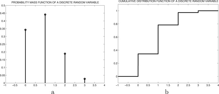
Figure 7.1: Illustration of the PMF and CDF of a simple discrete random variable in Example 7.2.1.

• A binomial random variable $X$ $X$ takes values in the set {0,1, 2,…, N} and could represent the number of Heads in N independent flips of a coin. If the probability of receiving a Head in each flip of the coin equals p, then the PMF of the binomial random variable is given by

$P χ (x) = (\begin{matrix} N \\ x \end{matrix}) p^{x} {(1 - p)}^{(N - x)}, 0 \leq x \leq N$ $P χ (x) = (\begin{matrix} N \\ x \end{matrix}) p^{x} {(1 - p)}^{(N - x)}, 0 \leq x \leq N$

(7.8)

Example 7.2.2. In error control coding, a rate 1/n repetitive code [6] consists of transmitting n identical copies of each bit. Let these bits be transmitted over a binary symmetric channel (BSC) with crossover probability p. In this case, random variable $X$ $X$ that represents the number of bits that are received correctly has the binomial distribution given in (7.8).

□

• A geometric random variable has a PMF of the form

$P χ (x) = {(1 - p)}^{x} p, x = 0, 1, 2, \dots$ $P χ (x) = {(1 - p)}^{x} p, x = 0, 1, 2, \dots$

(7.9)

Example 7.2.3. Consider a packet communication network in which a packet is retransmitted by the transmitter until a successful acknowledgment is received. In this case, if the probability of successful packet transmission in each attempt equals p and each transmission attempt is independent of the others, then random variable $X$ $X$ which represents the number of attempts until successful packet reception has a geometric distribution given in (7.9).

• A discrete uniform random variable $X$ $X$ has PMF of the form

$P χ (x) = \frac{1}{b - a + 1}, x = a, a + 1, \dots, b$ $P χ (x) = \frac{1}{b - a + 1}, x = a, a + 1, \dots, b$

(7.10)

where without loss of generality b ≥ a.

• A Pascal random variable has PMF

$P χ (x) = (\begin{matrix} N \\ x \end{matrix}) {(1 - p)}^{x} p, x = L, L + 1, L + 2, \dots$ $P χ (x) = (\begin{matrix} N \\ x \end{matrix}) {(1 - p)}^{x} p, x = L, L + 1, L + 2, \dots$

(7.11)

Consider a sequence of independent Bernoulli trials in which the probability of success in each trial equals p. The experiment is repeated until exactly L successes. The random variable $X$ $X$ that represents the number of trials has a Pascal distribution.

• A Poisson random variable has PMF of the form

$P χ (x) = e^{- a} \frac{a^{x}}{x!}, x = 0, 1, \dots$ $P χ (x) = e^{- a} \frac{a^{x}}{x!}, x = 0, 1, \dots$

(7.12)

The Poisson random variable is obtained as the limit of the binomial random variable in the limit that n → ∞ and p → 0 but the product np is a constant. The Poisson random variable represents the number of occurrences of an event in a given time period. For instance, the number of radioactive particles emitted in a given period of time by a radioactive source is modeled as a Poisson random variable. Similarly, in queueing theory a common model for packet arrivals is a Poisson process, in which the number of packet arrivals per unit time is given by (7.12).

□

7.2.2 Continuous Random Variables

Random variable $X$ $X$ is said to be a continuous random variable if the CDF of $X$ $X$ is continuous. The probability density function (PDF) $f_{X}$ $f_{X}$ (x) of random variable $X$ $X$ is defined as

$F χ (x) = \int_{- \infty}^{x} f χ (u) d u$ $F χ (x) = \int_{- \infty}^{x} f χ (u) d u$

(7.13)

Note that unlike the PMF, the PDF may take values greater than 1. The PDF is only proportional to the probability of an event. The interpretation of the PDF is that the probability of $X$ $X$ taking values between x and x + δ_x approximately equals $f_{X}$ $f_{X}$ (x)δ_x, for small positive values of δ_x. Similar to the CDF, the PDF is also a complete description of the random variable. The PDF of $X$ $X$ satisfies the following properties:

• Since the CDF is a nondecreasing function, the PDF is non-negative, i.e., $f_{X}$ $f_{X}$ (x) ≥ 0.

• The integral of the PDF over a certain interval represents the probability of the random variable taking values in that interval, i.e., $\int_{a}^{b} f_{X} (x) d x = \Pr (a < X \leq b)$ $\int_{a}^{b} f_{X} (x) d x = \Pr (a < X \leq b)$ .

• Extending the above property, the integral of the PDF over the entire range -TO equals 1, i.e., $\int_{- \infty}^{\infty} f_{X} (x) d x = 1$ $\int_{- \infty}^{\infty} f_{X} (x) d x = 1$ .

Example 7.2.4. Suppose a random point on the number line uniformly between the values 0 and 3. Let random variable $X$ $X$ represent the coordinate of that point. Then the PDF of $X$ $X$ is given by $f_{X} (x) = \frac{1}{3}$ $f_{X} (x) = \frac{1}{3}$ , 0 < x < 3. The corresponding CDF is given by

$F χ (x) = {\begin{array}{l} 0 & x \leq 0 \\ \frac{x}{3} & 0 < x < 3 \\ 1 & x \geq 3 \end{array}$ $F χ (x) = {\begin{array}{l} 0 & x \leq 0 \\ \frac{x}{3} & 0 < x < 3 \\ 1 & x \geq 3 \end{array}$

(7.14)

A plot of this PDF and CDF are given in Figure 7.2.

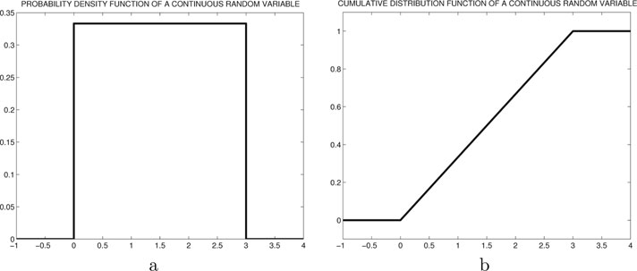
Figure 7.2: Illustration of the PMF and CDF of a simple discrete random variable in Example 7.2.4.

□

Similar to the discrete case, several commonly occurring continuous random variables have been studied including the following:

• The PDF of a uniform random variable is given by

$f χ (x) = \frac{1}{b - a}, x \in (a, b)$ $f χ (x) = \frac{1}{b - a}, x \in (a, b)$

(7.15)

• The PDF of a Gaussian random variable (also referred to as Normal random variable) is given by

$f χ (x) = \frac{1}{\sqrt{2 π σ^{2}}} e^{- \frac{{(x - μ χ)}^{2}}{2 σ^{2}}} .$ $f χ (x) = \frac{1}{\sqrt{2 π σ^{2}}} e^{- \frac{{(x - μ χ)}^{2}}{2 σ^{2}}} .$

(7.16)

The special case of a Gaussian random variable with 0 mean and unit variance is called a standard normal random variable. As will become clear in our study of the Central Limit Theorem, the distribution of any sum of independent random variables asymptotically approaches that of a Gaussian. Consequently, many noise and other realistic scenarios are modeled as Gaussian. The CDF of a Gaussian random variable is unfortunately not known in closed form. However, the CDF of a standard normal random variable has been computed numerically for various values and provided in the form of tables in several books. This CDF, denoted by Φ is defined as

$Φ (x) = \int_{- \infty}^{x} \frac{1}{\sqrt{2 π}} e^{- \frac{u^{2}}{2}} d u$ $Φ (x) = \int_{- \infty}^{x} \frac{1}{\sqrt{2 π}} e^{- \frac{u^{2}}{2}} d u$

(7.17)

The CDF of any other Gaussian random variable $X$ $X$ with mean $μ_{X}$ $μ_{X}$ and variance $σ_{X}^{2}$ $σ_{X}^{2}$ can be evaluated using the CDF tables of a standard normal random variable as follows

$\Pr (χ \leq x) = \int_{- \infty}^{x} \frac{1}{\sqrt{2 π σ_{χ}^{2}}} e^{- \frac{{(u - μ χ)}^{2}}{2 σ_{χ}^{2}}} d u = Φ (\frac{x - μ χ}{σ χ}) .$ $\Pr (χ \leq x) = \int_{- \infty}^{x} \frac{1}{\sqrt{2 π σ_{χ}^{2}}} e^{- \frac{{(u - μ χ)}^{2}}{2 σ_{χ}^{2}}} d u = Φ (\frac{x - μ χ}{σ χ}) .$

(7.18)

Note that several authors use other variants of Φ to numerically calculate the CDF and tail probabilities of a Gaussian random variable. For instance, the error function er f (x) is defined as

$e r f (x) = \frac{1}{\sqrt{π}} \int_{0}^{x} e^{- t^{2}} d t$ $e r f (x) = \frac{1}{\sqrt{π}} \int_{0}^{x} e^{- t^{2}} d t$

(7.19)

This error function er f (x) and the Φ function can be expressed in terms of each other as $Φ (x) = 0.5 + e r f (x / \sqrt{2})$ $Φ (x) = 0.5 + e r f (x / \sqrt{2})$ and $e r f (x) = Φ (x \sqrt{2} - 0.5)$ $e r f (x) = Φ (x \sqrt{2} - 0.5)$ for positive values of x.

• An exponential random variable has a PDF given by

$f χ (x) = a e^{- a x}, x > 0$ $f χ (x) = a e^{- a x}, x > 0$

(7.20)

The exponential distribution is frequently used to model the interarrival time between packets in the queueing theory (see Chapter 17). The exponential distribution has the special memoryless property as demonstrated by the following example.

Example 7.2.5. Let the lifetime of a fluorescent bulb be modeled as an exponential random variable $X$ $X$ with a mean of 10 years. Then the probability that the lifetime $X$ $X$ exceed 15 years is given by

$\Pr (X > 15) = \int_{x = 15}^{\infty} 1 / 10 e^{- x / 10} d x = e^{- 15 / 10}$ $\Pr (X > 15) = \int_{x = 15}^{\infty} 1 / 10 e^{- x / 10} d x = e^{- 15 / 10}$

(7.21)

Now suppose the bulb has already been working for 6 years. In this case, the conditional probability that the lifetime $X$ $X$ exceeds 15 years is given by

$\Pr (X > 15 / X > 6) = \frac{e^{- 15 / 10}}{e^{- 6 / 10}} = e^{- 9 / 10}$ $\Pr (X > 15 / X > 6) = \frac{e^{- 15 / 10}}{e^{- 6 / 10}} = e^{- 9 / 10}$

(7.22)

which is the same as the probability that the lifetime exceeds 15 − 6 = 9 years. The exponential random variable is the only continuous random variable that has this memoryless property.

□

7.3 Joint Random Variables

Recall that a random variable is a mapping from the set of outcomes of an experiment to real numbers. Clearly, for a given set of experimental outcomes, there could be numerous mappings representing different random variables to different sets of real numbers. To understand the relationships between the various random variables, it is not sufficient to study their properties independent of each other; a joint study of these random variables is required.

The joint CDF $F_{X, Y}$ $F_{X, Y}$ (x,y) of two random variables $X$ $X$ and $Y$ $Y$ is given by

$F_{χ, Y} (x, y) = \Pr (χ \leq x, Y \leq y)$ $F_{χ, Y} (x, y) = \Pr (χ \leq x, Y \leq y)$

(7.23)

Similar to the case of a single random variable, the joint CDF completely specifies the properties of the random variables. From the joint CDF, the marginal CDF of RVs $X$ $X$ and $X$ $X$ can be obtained as $F_{X}$ $F_{X}$ (x) = $F_{X, Y}$ $F_{X, Y}$ (x, ∞) and $F_{Y}$ $F_{Y}$ (y) = $F_{X, Y}$ $F_{X, Y}$ (∞,y). The joint CDF satisfies the following properties:

• 0 ≤ $F_{X, Y}$ $F_{X, Y}$ (x, y) ≤ 1.

• $F_{X, Y}$ $F_{X, Y}$ (−∞, −∞) = 0 and $F_{X, Y}$ $F_{X, Y}$ (∞, ∞) = 1.

• Pr (a < $X$ $X$ < b, c < $Y$ $Y$ ≤ d) = $F_{X, Y}$ $F_{X, Y}$ (a,c) + $F_{X, Y}$ $F_{X, Y}$ (b,d) − $F_{X, Y}$ $F_{X, Y}$ (a,d) − $F_{X, Y}$ $F_{X, Y}$ (b,c).

• $F_{X, Y}$ $F_{X, Y}$ (x, y) = lim_ϵ→0,ϵ>0 $F_{X, Y}$ $F_{X, Y}$ (x+ϵ, y) and $F_{X, Y}$ $F_{X, Y}$ (x, y) = lim_ϵ→0,ϵ>0 $F_{X, Y}$ $F_{X, Y}$ (x, y+ ϵ).

The joint PDF of RVs $X$ $X$ and $Y$ $Y$ is given by any function $F_{X, Y}$ $F_{X, Y}$ (x, y) such that

$F_{χ, Y} (x, y) = \int_{- \infty}^{x} \int_{- \infty}^{y} f χ, Y (u, v) d v d u$ $F_{χ, Y} (x, y) = \int_{- \infty}^{x} \int_{- \infty}^{y} f χ, Y (u, v) d v d u$

(7.24)

Example 7.3.1. Consider random variables $X$ $X$ and $Y$ $Y$ with joint PDF given by

$f χ, Y (x, y) = {\begin{array}{l} a (x + y + x y) & 0 \leq x \leq 1, 0 \leq y \leq 2 \\ 0 & else \end{array}$ $f χ, Y (x, y) = {\begin{array}{l} a (x + y + x y) & 0 \leq x \leq 1, 0 \leq y \leq 2 \\ 0 & else \end{array}$

(7.25)

The value of constant a =1/4 can be computed using the property that the integral of the PDF over the entire interval equals 1. In this case, the CDF can be computed as

$F_{χ, Y} (x, y) = {\begin{array}{l} 1 & x > 1, y > 2 \\ a (x^{2} y / 2 + y^{2} x / 2 + x^{2} y^{2} / 4) & 0 \leq x \leq 1, 0 \leq y \leq 2 \\ 0 & else \end{array}$ $F_{χ, Y} (x, y) = {\begin{array}{l} 1 & x > 1, y > 2 \\ a (x^{2} y / 2 + y^{2} x / 2 + x^{2} y^{2} / 4) & 0 \leq x \leq 1, 0 \leq y \leq 2 \\ 0 & else \end{array}$

(7.26)

The probability of various events can be computed either from the PDF or from the CDF. For example, let event A = {0 ≤ $X$ $X$ ≤ 1/2, 1 ≤ $Y$ $Y$ ≤ 2}. The probability of A can be calculated using the PDF as

$\Pr (A) = \int_{0}^{1 / 2} \int_{1}^{2} a (x + y + x y) d y d x$ $\Pr (A) = \int_{0}^{1 / 2} \int_{1}^{2} a (x + y + x y) d y d x$

(7.27)

$= a \int_{0}^{1 / 2} (x + 3 / 2 + 3 / 2 x) d x$ $= a \int_{0}^{1 / 2} (x + 3 / 2 + 3 / 2 x) d x$

(7.28)

$= 17 / 64$ $= 17 / 64$

(7.29)

The same probability can also be calculated using the joint CDF as

$\Pr (A) = F_{χ, Y} (1 / 2, 2) + F_{χ, Y} (0, 1) - F_{χ, Y} (0, 2) - F_{χ, Y} (1 / 2, 1)$ $\Pr (A) = F_{χ, Y} (1 / 2, 2) + F_{χ, Y} (0, 1) - F_{χ, Y} (0, 2) - F_{χ, Y} (1 / 2, 1)$

(7.30)

$= 3 / 8 + 0 - 0 - 7 / 64$ $= 3 / 8 + 0 - 0 - 7 / 64$

(7.31)

$= 17 / 64$ $= 17 / 64$

(7.32)

The marginal PDFs of $X$ $X$ and $Y$ $Y$ can now be computed as

$f χ (x) = \int_{y = 0}^{2} a (x + y + x y) d y = a (4 x + 2),$ $f χ (x) = \int_{y = 0}^{2} a (x + y + x y) d y = a (4 x + 2),$

(7.33)

$and f Y (y) = \int_{x = 0}^{1} a (x + y + x y) d x = a (3 y + 1) / 2.$ $and f Y (y) = \int_{x = 0}^{1} a (x + y + x y) d x = a (3 y + 1) / 2.$

(7.34)

□

The conditional PDF $f_{X | Y}$ $f_{X | Y}$ (x∣y) is defined as

$f_{χ | Y} (x | y) = \frac{f χ, Y (x, y)}{f Y (y)}$ $f_{χ | Y} (x | y) = \frac{f χ, Y (x, y)}{f Y (y)}$

(7.35)

when $f_{Y}$ $f_{Y}$ (y) > 0. For instance, in Exercise 7.3.1, the conditional PDF $f_{X | Y} (x | y) = \frac{2 (x + y + x y)}{3 y + 1}$ $f_{X | Y} (x | y) = \frac{2 (x + y + x y)}{3 y + 1}$ , 0<x<1 and conditional PDF $f_{X | Y} (y | x) = \frac{(x + y + x y)}{4 x + 2}$ $f_{X | Y} (y | x) = \frac{(x + y + x y)}{4 x + 2}$ , 0<y<1. Continuous random variables $X$ $X$ and $Y$ $Y$ are said to be independent if and only if

$\begin{matrix} f_{χ,}_{_{Y}} (x, y) = f_{χ} (x) f_{Y} (y), & \forall x, y . \end{matrix}$ $\begin{matrix} f_{χ,}_{_{Y}} (x, y) = f_{χ} (x) f_{Y} (y), & \forall x, y . \end{matrix}$

7.36

Example 7.3.2. Let the joint PDF of random variables $X$ $X$ and $Y$ $Y$ be given by $f_{X, Y}$ $f_{X, Y}$ (x, y) = xy for 0 ≤ x ≤ 1,0 ≤ y ≤ 2. Then the corresponding marginal PDFs are given by $f_{X} (x) = \int_{y = 0}^{2} x y d y = 2 x$ $f_{X} (x) = \int_{y = 0}^{2} x y d y = 2 x$ , 0 ≤ x ≤ 1 and $f_{Y} (y) = \int_{x = 0}^{2} x y d x = y / 2$ $f_{Y} (y) = \int_{x = 0}^{2} x y d x = y / 2$ , 0 ≤y ≤ 2. Clearly, $f_{X, Y}$ $f_{X, Y}$ (x,y) = $f_{X}$ $f_{X}$ (x) $f_{Y}$ $f_{Y}$ (y), which implies that random variables $X$ $X$ and $Y$ $Y$ are independent.

□

Similarly, discrete random variables $X$ $X$ and $Y$ $Y$ are said to be independent if and only if

$P_{χ, Y} (x, y) = P_{χ} (x) P_{Y} (y), \forall x, y$ $P_{χ, Y} (x, y) = P_{χ} (x) P_{Y} (y), \forall x, y$

(7.37)

It is important to note that for independence of random variables (7.37) needs to be satisfied for all values of the random variables $X$ $X$ and $Y$ $Y$ .

Example 7.3.3. Let the joint PMF of random variables $X$ $X$ and $Y$ $Y$ be given by

$P_{χ, Y} (x, y) = {\begin{array}{l} 1 / 6 & χ = 1, Y = 1 \\ 1 / 4 & χ = 1, Y = 2 \\ 1 / 12 & χ = 1, Y = 3 \\ 1 / 6 & χ = 2, Y = 1 \\ 1 / 12 & χ = 1, Y = 2 \\ 1 / 4 & χ = 1, Y = 3 \end{array}$ $P_{χ, Y} (x, y) = {\begin{array}{l} 1 / 6 & χ = 1, Y = 1 \\ 1 / 4 & χ = 1, Y = 2 \\ 1 / 12 & χ = 1, Y = 3 \\ 1 / 6 & χ = 2, Y = 1 \\ 1 / 12 & χ = 1, Y = 2 \\ 1 / 4 & χ = 1, Y = 3 \end{array}$

(7.38)

The marginal PMFs of $X$ $X$ and $Y$ $Y$ can be computed to show that they are both uniform densities over their respective alphabets. In this case, it can be easily verified that the events $X$ $X$ = 1 and $Y$ $Y$ =1 are independent. However, the events $X$ $X$ = 1 and $Y$ $Y$ = 2 are not independent. Thus, the random variables $X$ $X$ and $Y$ $Y$ are not independent.

Example 7.3.4. Consider a network in which packets are routed from the source node to the destination node using a routing protocol. Let there also be a probability a of packet loss at each node due to buffer overflows or errors in the link. In order to increase the overall chances of success, the routing algorithm sends three copies of each packet over different mutually exclusive routes. The three routes have a₁, a₂ and a₃ hops between the source and destination, respectively. Assume that the probability of success in each hop is independent of the other hops. In this case the overall probability that at least one copy of the packet is received correctly at the destination node can be calculated as $1 - \prod_{i = 1}^{3} (1 - (1 -) {(1 - α)}^{α_{i}})$ $1 - \prod_{i = 1}^{3} (1 - (1 -) {(1 - α)}^{α_{i}})$ .

□

7.3.1 Expected Values, Characteristic Functions

As noted before, the PDF, CDF and PMF are all complete descriptors of the random variable and can be used to evaluate any property of the random variable. However, for many complex scenarios, computing the exact distribution can be challenging. In contrast, there are several statistical values that are computationally simple, but provide only partial information about the random variable. In this section, we highlight some of the frequently utilized statistical measures.

The expected value, E { $X$ $X$ }, of random variable $X$ $X$ is defined as

$E {χ} = μ_{χ} = \int x f χ (x) d x$ $E {χ} = μ_{χ} = \int x f χ (x) d x$

(7.39)

In general the expected value of any function g( $X$ $X$ ) of a random variable $X$ $X$ is given by

$E {g (χ)} = \int g (x) f χ (x) d x$ $E {g (χ)} = \int g (x) f χ (x) d x$

(7.40)

The term, E { $X^{k}$ $X^{k}$ } is known as the k^th moment of $X$ $X$ . The variance $σ_{X}^{2}$ $σ_{X}^{2}$ of $X$ $X$ is related to the second moment and is given by

$σ_{χ}^{2} = E {{(χ - μ_{χ})}^{2}} = E {χ^{2}} - μ_{χ}^{2}$ $σ_{χ}^{2} = E {{(χ - μ_{χ})}^{2}} = E {χ^{2}} - μ_{χ}^{2}$

(7.41)

As another variation, the k^th central moment of random variable is defined as $E {{(X - μ_{X})}^{k}}$ $E {{(X - μ_{X})}^{k}}$ .

The covariance between random variables $X$ $X$ and $Y$ $Y$ is defined as

$C o v (χ, Y) = E {(χ - μ_{χ}) (Y - μ_{Y})}$ $C o v (χ, Y) = E {(χ - μ_{χ}) (Y - μ_{Y})}$

(7.42)

The correlation coefficient $ρ_{X Y}$ $ρ_{X Y}$ is defined as

$ρ χ, Y = \frac{E {(χ - μ_{χ}) (Y - μ_{Y})}}{σ_{χ} σ_{Y}}$ $ρ χ, Y = \frac{E {(χ - μ_{χ}) (Y - μ_{Y})}}{σ_{χ} σ_{Y}}$

(7.43)

Example 7.3.5. Jointly Gaussian Vector The joint PDF of the Gaussian vector $[X_{1}, X_{2}, \dots X_{N}]$ $[X_{1}, X_{2}, \dots X_{N}]$ is given by

$f χ_{1}_{,} χ_{2, \dots,} χ_{n} (x_{1}, x_{2}, \dots x_{n}) = \frac{1}{{(2 π)}^{N / 2} {| R χ |}^{1 / 2}} e^{- \frac{1}{2} {(x - μ_{x})}^{T} R_{χ}^{- 1} (x - μ_{x})}$ $f χ_{1}_{,} χ_{2, \dots,} χ_{n} (x_{1}, x_{2}, \dots x_{n}) = \frac{1}{{(2 π)}^{N / 2} {| R χ |}^{1 / 2}} e^{- \frac{1}{2} {(x - μ_{x})}^{T} R_{χ}^{- 1} (x - μ_{x})}$

(7.44)

where x = [x₁, x₂,… x_n]^T and μ_X = ${[μ_{X_{1}} μ_{X_{1}} \dots μ_{X_{N}}]}^{T}$ ${[μ_{X_{1}} μ_{X_{1}} \dots μ_{X_{N}}]}^{T}$ is the mean of the different random variables and $R_{X}$ $R_{X}$ is the covariance matrix with i^th row and j^th column element given by Cov $(X_{i}, X_{j})$ $(X_{i}, X_{j})$ . Gaussian random vectors are frequently used in several signal processing applications. For instance, when estimating a vector parameter in the presence of additive noise. The reasons for the popularity of these Gaussian vector models are: i) by central limit theorem, the noise density is well approximated as a Gaussian, ii) several closed form analytical results can be derived using the Gaussian model, and iii) the results derived using a Gaussian approximation serves as a bound for the true performance.

The marginal density of a jointly Gaussian vector are a Gaussian random variable. However, marginal densities being Gaussian does not necessarily imply that the joint density is also Gaussian.

□

The random variables $X$ $X$ and $Y$ $Y$ are said to be uncorrelated if $ρ X, Y$ $ρ X, Y$ = 0. If $X$ $X$ and $Y$ $Y$ are independent, then

$E {(χ - μ_{χ}) (Y - μ_{Y})} = E {χ - μ_{χ}} E {Y - μ_{Y}} = 0,$ $E {(χ - μ_{χ}) (Y - μ_{Y})} = E {χ - μ_{χ}} E {Y - μ_{Y}} = 0,$

(7.45)

which implies that the random variables are also uncorrelated. However, uncorrelated random variables are not always independent as demonstrated by the following example.

Example 7.3.6. Let $X_{1}$ $X_{1}$ be uniformly distributed in the interval (0, 2π). Let $X_{2}$ $X_{2}$ = cos( $X_{1}$ $X_{1}$ ) and $X_{3}$ $X_{3}$ = sin( $X_{1}$ $X_{1}$ ). Then it is clear that $μ_{X_{2}} = μ_{X_{2}} = 0$ $μ_{X_{2}} = μ_{X_{2}} = 0$ and E ${X_{2}, X_{3}}$ ${X_{2}, X_{3}}$ = 0. Consequently, $ρ X_{2}, Y_{3}$ $ρ X_{2}, Y_{3}$ = 0. However, it is clear that $X_{2}$ $X_{2}$ and $X_{3}$ $X_{3}$ are dependent random variables since $X_{2}^{2} + X_{3}^{2} = 1$ $X_{2}^{2} + X_{3}^{2} = 1$ and given the value of $X_{2}$ $X_{2}$ the value of $X_{3}$ $X_{3}$ is known except for its sign.

□

In the special case that $X_{2}$ $X_{2}$ and $X_{2}$ $X_{2}$ are jointly Gaussian, then if they are uncorrelated they are also independent. This result can be verified by plugging in crosscorrelation values of 0 in the autocorrelation matrix $R_{X}$ $R_{X}$ that determines the joint PDF of $X_{2}$ $X_{2}$ and $X_{3}$ $X_{3}$ . Matrix R becomes a diagonal matrix and consequently the joint PDF then simply becomes the product of the marginal PDFs.

The characteristic function $ϕ_{X} (ω)$ $ϕ_{X} (ω)$ of $X$ $X$ is defined as

$ϕ χ (ω) = E {e^{j ω χ}} = \int f χ (x) e^{j ω x} d x$ $ϕ χ (ω) = E {e^{j ω χ}} = \int f χ (x) e^{j ω x} d x$

(7.46)

The characteristic function and the PDF form a unique pair; thus, the characteristic function also completely defines the random variable.

The characteristic function can be used to easily compute the moments of the random variable. Using the Taylors series expansion of e^jωx, we can expand the characteristic function as

$ϕ χ (ω) = E {e^{j ω χ}}$ $ϕ χ (ω) = E {e^{j ω χ}}$

(7.47)

$= E {1 + j ω x + \frac{{(j ω x)}^{2}}{2!} + \dots}$ $= E {1 + j ω x + \frac{{(j ω x)}^{2}}{2!} + \dots}$

(7.48)

$= 1 + j ω E {χ} + \frac{{(j ω)}^{2}}{2!} E {χ^{2}} + \dots$ $= 1 + j ω E {χ} + \frac{{(j ω)}^{2}}{2!} E {χ^{2}} + \dots$

(7.49)

Now to compute the k^th moment $E {X^{k}}$ $E {X^{k}}$ , we can differentiate (7.49) k times with respect to ω and then evaluate the result at ω = 0. Thus, $E {X^{k}} \frac{1}{j^{k}} \frac{d^{k}}{d ω^{k}} ϕ_{X} (ω)$ $E {X^{k}} \frac{1}{j^{k}} \frac{d^{k}}{d ω^{k}} ϕ_{X} (ω)$ .

Example 7.3.7. Let $X$ $X$ be an exponential random variable with parameter λ. The characteristic function of this random variable $X$ $X$ is given by

$\begin{array}{l} ϕ χ (ω) = E {e^{j ω x}} & = & \int f χ (x) e^{j ω x} d x \\ = & \int_{0}^{\infty} λ e^{- λ x} e^{j ω x} d x \\ = & \frac{λ}{λ - j ω} . \end{array}$ $\begin{array}{l} ϕ χ (ω) = E {e^{j ω x}} & = & \int f χ (x) e^{j ω x} d x \\ = & \int_{0}^{\infty} λ e^{- λ x} e^{j ω x} d x \\ = & \frac{λ}{λ - j ω} . \end{array}$

(7.50)

The mean of $X$ $X$ can be calculated as

$μ χ = \frac{1}{j} \frac{d}{d ω} ϕ χ (ω) {|_{ω = 0} = \frac{1}{j} \frac{λ j}{{(λ - j ω)}^{2}} |}_{ω = 0} = \frac{1}{λ}$ $μ χ = \frac{1}{j} \frac{d}{d ω} ϕ χ (ω) {|_{ω = 0} = \frac{1}{j} \frac{λ j}{{(λ - j ω)}^{2}} |}_{ω = 0} = \frac{1}{λ}$

(7.51)

The second order moment can be evaluated as

$E {χ^{2}} = \frac{1}{j^{2}} \frac{d}{d ω^{2}} ϕ χ (ω) {|_{ω = 0} = \frac{1}{j^{2}} \frac{- 2 λ}{{(λ - j ω)}^{3}} |}_{ω = 0} = \frac{2}{λ^{2}}$ $E {χ^{2}} = \frac{1}{j^{2}} \frac{d}{d ω^{2}} ϕ χ (ω) {|_{ω = 0} = \frac{1}{j^{2}} \frac{- 2 λ}{{(λ - j ω)}^{3}} |}_{ω = 0} = \frac{2}{λ^{2}}$

(7.52)

Consequently, the variance can be calculated as

$σ_{χ}^{2} = E {χ^{2}} - μ_{χ}^{2} = \frac{1}{λ^{2}}$ $σ_{χ}^{2} = E {χ^{2}} - μ_{χ}^{2} = \frac{1}{λ^{2}}$

(7.53)

The second characteristic function $ψ_{X} (ω)$ $ψ_{X} (ω)$ is defined as the natural logarithm of the function $ϕ_{X} (ω)$ $ϕ_{X} (ω)$ . The cumulants λ_n are

□

$λ_{n} = \frac{d Ψ (s)}{d s^{n}} | s = 0$ $λ_{n} = \frac{d Ψ (s)}{d s^{n}} | s = 0$

(7.54)

The various cumulants are related to the moments as follows:

$λ_{1} = E {χ} = μ χ$ $λ_{1} = E {χ} = μ χ$

(7.55)

$λ_{2} = E {{(χ - E {χ})}^{2}} = σ_{χ}^{2}$ $λ_{2} = E {{(χ - E {χ})}^{2}} = σ_{χ}^{2}$

(7.56)

$λ_{3} = E {{(χ - E {χ})}^{3}}$ $λ_{3} = E {{(χ - E {χ})}^{3}}$

(7.57)

$\begin{array}{l} λ_{4} = E {χ^{4}} - 4 E {χ^{3}} E {χ} \\ - 3 {(E {χ^{2}})}^{2} + 12 E {χ^{2}} {(E {χ})}^{2} - 6 {(E {χ})}^{4} \end{array}$ $\begin{array}{l} λ_{4} = E {χ^{4}} - 4 E {χ^{3}} E {χ} \\ - 3 {(E {χ^{2}})}^{2} + 12 E {χ^{2}} {(E {χ})}^{2} - 6 {(E {χ})}^{4} \end{array}$

(7.58)

The cumulants of order higher than 3 are not the same as the central moment. Of special interest is the fourth-order cumulant, which is also referred to as kurtosis. The kurtosis is typically used as a measure of the deviation from Gaussianity of a random variable. The kurtosis of a Gaussian random variable equals 0. Further, for a distribution with a heavy tail and a peak at zero, the kurtosis is positive and for distribution with a fast decaying tail the kurtosis is negative.

Example 7.3.8. Consider the uniform random variable $X$ $X$ with support over (0,1). The first four moments of $X$ $X$ can be calculated as

$E {χ} = 0, E {χ^{2}} = 1 / 12, E {χ^{3}} = 0, and E {χ^{4}} = 1 / 80$ $E {χ} = 0, E {χ^{2}} = 1 / 12, E {χ^{3}} = 0, and E {χ^{4}} = 1 / 80$

The kurtosis of $X$ $X$ can be now calculated using (7.58) as λ₄ = −2/15.

□

..................Content has been hidden....................

You can't read the all page of ebook, please click here login for view all page.

Table of Contents for 7 Probability, Random Variables, and Stochastic Processes

Create new playlist

Sign In

Sign Up

Table of Contents for
7 Probability, Random Variables, and Stochastic Processes