Chapter 17  Queueing Theory

Thomas Chen^‡

‡ Swansea University, Wales, UK

17.1    Introduction

Queueing theory has been successful for performance analysis of circuit-switched and packet-switched networks. Historically, queueing theory can be traced back to Danish mathematician A. K. Erlang who developed the well-known Erlang B and Erlang C formulas relating the capacity of telephone switches to the probability of call blocking. Since the emergence of packet switching in the late 1960s, queueing theory has become the primary mathematical apparatus for modeling and analysis of computer networks including the Internet. For packet-switched networks, the main performance metrics of interest are usually packet loss and packet delays.

Simple and intermediate queueing theory is centered mainly around queueing systems with Poisson arrivals, which can be treated relatively easily by Markov chains. For practical problems, the accuracy of these queueing models is often debatable. Unfortunately, more realistic queueing systems tend to become much more complicated and intractable (in advanced queueing theory).

17.2    Markov Chains

A brief review of Markov chains is a useful prologue to queueing theory. Recall from Chapter 6 that Markov processes are a class of stochastic processes that have the Markov (memoryless) property: the future evolution of a Markov process depends only on the current state and not on previous states. In other words, given the history of the process, the future depends only on the most recent state. For a Markov process, it is not necessary to know the entire history of the process in order to predict its future values; only the most recent point is sufficient.

Definition 17.2.1. For a discrete-time process X_n, the Markov property is

$Pr\left(X_{n=1}\le x|X_n=x_n,X_{n-1}=x_{n-1,\dots }\right)=Pr\left(X_{n+1}\le x|X_n=x_n\right)$

(17.1)

For a continuous-time process X_t, the Markov property is

$Pr\left(X_t\le x|X_{s,}s\le 0\right)=Pr\left(X_t\le x|X_0\right)$

(17.2)

for t ≥ 0.

Markov chains are a subset of Markov processes with discrete states, usually associated with integers without loss of generality. Markov chains can be discretetime making a transition at every time increment or continuous-time making state transitions at random times. The Markov property implies that the next state change depends only on the current state and not on previous history (i.e., how it got to that state).

17.2.1    Discrete-Time Markov Chains

A discrete-time Markov chain can be characterized by a (one-step) transition probability matrix

$P=\left[\begin{array}{llll}{p}_{00}\hfill & p_{01}\hfill & p_{02}\hfill & \cdots \hfill \\ p_{10}\hfill & p_{11}\hfill & p_{12}\hfill & \cdots \hfill \\ :\hfill & :\hfill & :\hfill & :\hfill \end{array}\right]$

(17.3)

where the matrix elements are the transition probabilities

$p_{ij}=P\left(X_{n+1}=j|X_n=i\right)$

(17.4)

for all states i, j. The transition (probability) matrix is infinite size if the number of possible states is infinite.

Queueing theory is usually interested in the steady-state or equilibrium of a Markov chain. Not every Markov chain has a steady-state distribution, but the Markov chains encountered in elementary queueing theory will have one. It means that if the Markov chain goes for a long time, then the probability of X_n = i will approach some steady-state probability π_i that is independent of the chain’s initial state. In another interpretation, if the Markov chain starts in the steady-state distribution at time 0, it will continue indefinitely with these probabilities. In addition, if the Markov chain is observed over a very long time, the relative fraction of time spent in state i will be π_i.

Theorem 17.2.1. If the steady-state probabilities denoted by the vector π = [π₀ π₁ ⋯] exist for a discrete-time Markov chain, they can be found as the unique solution to the balance equations:

$\pi =\pi P$

(17.5)

or

${\pi }_j={\displaystyle \sum _i{\pi }_i{p}_{ij}}$

(17.6)

under the constraint that the probabilities must sum to one, Σ_i π_i = 1.

17.2.2    Continuous-Time Markov Chains

Unlike discrete-time Markov chains, continuous-time Markov chains can make state transitions at random times. A discrete-time Markov chain can be found embedded in a continuous-time Markov chain.

Theorem 17.2.2. For a continuous-time Markov chain X_t with transition times {t₁, t₂, …}, the points $Y_n=X_{t_n}$ constitute an embedded discrete-time Markov chain. Given the current state Y_n = i, the time spent in the state τ_n = t_n+1 − t_n is exponentially distributed with some parameter a_i dependent only on the current state i.

Definition 17.2.2. The transition rate from current state i to another state j is governed by the infinitessimal rates

$a_{ij}=a_{i}P\left(Y_{n+1}=j|Y_n=i\right)$

(17.7)

The infinitessimal rate a_ij implies that the time spent in state i until a transition is made to state j is exponentially distributed with mean 1/a_ij. The conditional rate matrix

$A=\left[\begin{array}{llll}{p}_{00}\hfill & p_{01}\hfill & p_{02}\hfill & \cdots \hfill \\ p_{10}\hfill & p_{11}\hfill & p_{12}\hfill & \cdots \hfill \\ :\hfill & :\hfill & :\hfill & :\hfill \end{array}\right]$

(17.8)

is analogous to the transition probability matrix P for discrete-time Markov chain in that A completely characterizes a continuous-time Markov chain.

Theorem 17.2.3. If a continuous-time Markov chain has steady-state or equilibrium probabilities {π_i}, then they are the unique solutions of the balance equations

$a_j{\text{π}}_j={\displaystyle \sum _{i\ne j}{\text{π}}_i{a}_{ij}}$

(17.9)

under the constraint that the probabilities must sum to one, Σ_i π_i = 1.

The balance equations can be written compactly in matrix form as simply

$0=\text{π}Q$

(17.10)

where the Q matrix is defined as

$Q\equiv \left[\begin{array}{lllll}-a_0\hfill & a_{01}\hfill & a_{02}\hfill & a_{03}\hfill & \cdots \hfill \\ a_{10}\hfill & -a_1\hfill & a_{12}\hfill & a_{13}\hfill & \cdots \hfill \\ a_{20}\hfill & a_{21}\hfill & a_2\hfill & a_{23}\hfill & \cdots \hfill \\ a_{30}\hfill & a_{31}\hfill & a_{32}\hfill & -a_3\hfill & \cdots \hfill \\ :\hfill & :\hfill & :\hfill & :\hfill & \cdots \hfill \end{array}\right]$

(17.11)

Poisson Counting Process

The Poisson counting process is a continuous-time Markov chain of special interest to queueing theory. The conditional rate matrix is

$A=\left[\begin{array}{llll}0\hfill & \text{λ}\hfill & 0\hfill & \cdots \hfill \\ 0\hfill & 0\hfill & \text{λ}\hfill & \ddots \hfill \\ 0\hfill & 0\hfill & 0\hfill & \ddots \hfill \\ ⋮\hfill & \ddots \hfill & \ddots \hfill & \ddots \hfill \end{array}\right]$

(17.12)

Alternatively, the Poisson counting process can be characterized by its transition times. Imagine a series of arrivals (or “births”) at times t_i for the ith arrival starting from time 0, where interarrival times are independent and exponentially distributed with parameter λ. The point process {t₁, t₂, …} is called a Poisson arrival process. The Poisson counting process X_t is the number of arrivals up to time t. It is called Poisson because X_t for any given t is a Poisson random variable with the probability mass function:

$Pr\left(X_t=k\right)=\frac{{\left(\text{λ}t\right)}^k}{k!}{e}^{-\text{λ}t}$

(17.13)

for k = 0, 1, … In fact, the number of arrivals in any time interval (s, s + t) is Poisson with mean λt.

A third way to look at the process is to consider a time interval (0, t) and divide it into short intervals of length Δ. In each short interval, either there is an arrival with probability λΔ or no arrival with probability 1 − λΔ. Arrivals in each short interval is a Bernoulli trial, and assume the short intervals are all independent. It is evident that the number of arrivals in the interval (0, t) has a binomial distribution with mean At. Shrinking the short intervals in the limit Δ → 0 however, the number of trials becomes infinite while the mean number of arrivals is fixed; the binomial distribution is known to approach the Poisson distribution in this case.

This third view of the Poisson arrival process is interesting because its “memoryless property” (of particular importance to queueing theory) becomes clear. Suppose that we know the last arrival occurred at time −T, hence no arrivals have occurred up to time 0. When will the next arrival occur? By the method of construction, every short interval is independent, and therefore the time to the next arrival will be independent of the previous arrival time, i.e., the next arrival time will be exponentially distributed with parameter λ regardless of T.

This constructive view is also useful to show another interesting property of the Poisson arrival process. Consider the aggregate of two independent Poisson arrival processes, one with rate λ₁ and the other with λ₂ . Again, consider a time interval (0, t) divided into short intervals of length Δ. The probability of two arrivals in an interval is λ₁λ₂Δ² but this becomes negligible in the limit Δ → 0. Only the probability of one arrival, (λ₁ + λ₂)Δ, is significant. Taking the limit, it becomes clear that the aggregate of two independent Poisson arrival processes is itself a Poisson arrival process with rate λ₁ + λ₂. Similarly, it can be shown by reversing the argument that random splitting of a Poisson arrival process will result in two independent Poisson arrival processes.

Birth-Death Process

Generally, a population can have random births (arrivals) and deaths (departures). A birth-death process is a continuous-time Markov chain often encountered in queueing theory. Its state transition diagram showing infinitessimal rates between consecutive states is shown in Figure 17.1. If the population is in state i, the time to the next birth is exponentially distributed with parameter λ_i while the time to the next death is exponentially distributed with parameter μ_i. The conditional rate matrix is

$A=\left[\begin{array}{lllll}0\hfill & {\text{λ}}_0\hfill & 0\hfill & 0\hfill & \cdots \hfill \\ {\mu }_1\hfill & 0\hfill & {\text{λ}}_1\hfill & 0\hfill & \ddots \hfill \\ 0\hfill & {\mu }_2\hfill & 0\hfill & {\text{λ}}_2\hfill & \ddots \hfill \\ ⋮\hfill & \ddots \hfill & \ddots \hfill & \ddots \hfill & \ddots \hfill \end{array}\right]$

(17.14)

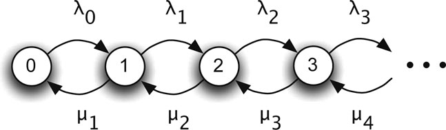
Figure 17.1:  Birth-death process.

In order to find steady-state probabilities, one could use the balance equation 0 = πQ, but consider an intuitive argument. In steady-state, we would expect that the total transition rates in opposite directions between states 0 and 1 should be equal, leading to the first balance equation

${\text{λ}}_0{\text{π}}_0={\mu }_1{\text{π}}_1$

(17.15)

Likewise, considering the transition rates in opposite directions between states 1 and 2 leads to the next balance equation

${\text{λ}}_{\text{1}}{\text{π}}_1={\mu }_2{\text{π}}_2$

(17.16)

In general, it can be seen that

${\text{λ}}_j{\text{π}}_j={\mu }_{j+1}{\text{π}}_{j+1}$

(17.17)

for all j. Along with the additional constraint π₀ + π₁ + ⋯ = 1, if a unique solution exists to the balance equations, then the steady-state probabilities for the birth-death process are

$\begin{array}{l}{\text{π}}_0={\left({\displaystyle \sum _j\frac{{\text{λ}}_0\cdots {\text{λ}}_{j-1}}{{\mu }_1\cdots {\mu }_j}}\right)}^{-1}\\ {\text{π}}_j=\frac{{\text{λ}}_0\cdots {\text{λ}}_{j-1}}{{\mu }_1\cdots {\mu }_j}{\text{π}}_0,j>0\end{array}$

(17.18)

17.3    Queueing Models

Queueing theory is a branch of applied probability dealing with “customers” or “jobs” that require service or otherwise wait in buffers. In packet networks, customers are packets and service consists of the time to transmit a packet on a link. The simplest system is a single-server queue as shown in Figure 17.2. An arriving customer wants to occupy the server for a service time. When the server is busy, any new arrivals must join the queue. When the server becomes free, a customer from the queue enters into service. After a service time, the customer departs the system. The operation of the system depends on the random arrival process and the random service times.

Figure 17.2:  A single-server queue.

It is easy to imagine more complicated queueing systems involving multiple queues or multiple servers. The queues may use various service disciplines such as priorities. The server might allow preemption (service interruption) and retries. Multiple queueing systems may work in parallel or series.

In general, the analysis of packet networks involves three performance metrics of interest:

•  the delay through the system which is the sum of the waiting time in the queue and the service time;

•  the number in the system which is the sum of the number waiting in the queue (queue length) and the number in service;

•  the probability of losing customers if the buffer capacity is finite.

Typically, several assumptions are understood implicitly unless a different assumption is stated explicitly. These implicit assumptions include:

•  customers arrive singly unless batch arrivals are specified;

•  a server handles one customer at a time unless batch service is specified;

•  the service discipline is FIFO (first in first out) also known as FCFS (first come first served);

•  the buffer has infinite capacity;

•  once queued, arrivals do not defect from the queue before receiving service or jump between queues (in the case of multiple queues);

•  if the buffer is finite, arrivals are dropped from the tail of the queue;

•  service is non-preemptive meaning that a customer in service must complete service without interruption;

•  the system is work conserving meaning that a server cannot stand idle if any customers are waiting, and customers do not duplicate any completed service.

Traditional queueing models assume that arrivals are a renewal process, i.e., interarrival times are independent and identically distributed (i.i.d.) with a known probability distribution function A(t). By convention, λ refers to the mean arrival rate implying that 1/λ is the mean interarrival time. In addition, service times are also i.i.d. with a known service time probability distribution function B(t). By convention, μ is the service rate, or 1/μ is the mean service time. The utilization or load factor is the ratio of mean service time to mean interarrival time, ρ = λ/μ. For single-server queues, ρ is the fraction of time that the system is busy. Normally, performance analysis is interested in the stable case ρ < 1. When ρ > 1, the queue length grows without bounds.

Since a complete description of a queueing model would be lengthy, statistician David Kendall suggested a shorthand notation having the form A/B/C which can be expanded to a longer form A/B/C/D/E/F. The concise form of A/B/C is understood to mean that the other parameters have their default values. The parts of the notation have the meanings listed below.

A	Probability distribution function for interarrival time
B	Probability distribution function for service time
C	Number of servers
D	Maximum capacity of system including server (infinite by default)
E	Total population of customers (infinite by default)
F	Service discipline (FIFO by default)

Because certain probability distribution functions arise commonly for interarrival times and service times, there is shorthand notation to refer to common probability distributions:

M	Exponential
D	Deterministic
Ek	Erlang with parameter k
G	General

17.4    M/M/1 Queue

The simplest queue is the M/M/1 queue, meaning a single-server queue with Poisson arrivals and exponential service times. Poisson arrivals with mean rate λ means that interarrival times are i.i.d. according to an exponential probability density function with mean 1/λ:

$p\left(t\right)=\text{λ}{e}^{-\text{λ}t}$

(17.19)

The service times are i.i.d. according to another exponential probability density function with mean 1/μ:

$p\left(s\right)=\mu e^{-\mu \text{s}}$

(17.20)

The M/M/1 queue is the simplest to analyze because the system state is captured completely by the number in the system, X_t, which is a simple birth-death process. However, some explanation is necessary to justify why the number in the system is sufficient to represent the entire system state. For a general queueing system, the complete system state would need to include three variables:

•  the number in the system, X_t;

•  the time that the current customer has already spent in service, Y_t;

•  the time since the last arrival, Z_t.

The next change in X_t will be either an arrival or departure. The time since the current customer began service, Y_t, is important because it affects the next departure time. Generally, the customer’s remaining service time depends on how much service has already been spent. The time since the last arrival, Z_t, is important because it affects the next arrival time. Hence, the triplet (X_t, Y_t, Z_t) captures the state of the system at time t sufficiently to determine the future behavior of the system.

For the M/M/1 queue, the Poisson arrival process is memoryless and exponential service times are memoryless. By the memoryless property of Poisson arrivals, the time to the next arrival will be exponentially distributed regardless of the time since the last arrival. Hence, Y_t is not relevant to the future behavior of X_t. Similarly, the current customer’s remaining service time will be exponentially distributed regardless of how much service the customer has already received. It is unnecessary to examine Z_t to predict the next departure. Hence, knowledge of the number in the system X_t is sufficient to predict future changes in the M/M/1 queue.

17.4.1    Steady-State Probabilities for Number in System

The number in the system, X_t, will change by the next arrival or departure. The time to the next arrival will be exponentially distributed with parameter λ, and if X_t > 0, the time to the next departure will be exponentially distributed with parameter μ. Hence, X(t) is a birth-death process with birth rates λ and death rates μ represented by the state transition diagram shown in Figure 17.3 and the conditional rate matrix

$A=\left[\begin{array}{lllll}0\hfill & \text{λ}\hfill & 0\hfill & 0\hfill & \cdots \hfill \\ \mu \hfill & 0\hfill & \text{λ}\hfill & 0\hfill & \ddots \hfill \\ 0\hfill & \mu \hfill & 0\hfill & \text{λ}\hfill & \ddots \hfill \\ ⋮\hfill & \ddots \hfill & \ddots \hfill & \ddots \hfill & \ddots \hfill \end{array}\right]$

(17.21)

The steady-state probabilities {π_i} for X_t are found in the usual way from the balance equations:

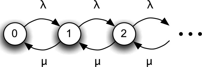
Figure 17.3:  State transition diagram for X(t).

$\begin{array}{lll}{\text{λπ}}_0\hfill & =\hfill & \mu {\text{π}}_1\hfill \\ {\text{λπ}}_1\hfill & =\hfill & \mu {\text{π}}_2\hfill \\ {\text{λπ}}_2\hfill & =\hfill & \mu {\text{π}}_3\hfill \\ \hfill & :\hfill & \hfill \end{array}$

(17.22)

with the additional constraint that all probabilities must sum to one: π₀+ π₁•+• • = 1. Putting all probabilities in terms of π₀, we get the general relation

${\text{π}}_j={\rho }^j{\text{π}}_0$

(17.23)

By substitution, we find the solution is the geometric probabilities:

${\text{π}}_j={\rho }^j\left(1-\rho \right)$

(17.24)

for j = 0, 1, …

The stability condition ρ < 1 is easy to see. If ρ > 1, there is no possible solution to the balance equations because the queue length will eventually drift to infinity. The non-obvious condition is ρ = 1. Intuitively, it might seem reasonable to expect the queue to be stable if the arrival rate is equal to the service rate. However, the balance equations become π₀ = π₁ = π₂ ⋯ and at the same time, an infinite number of equal probabilities sum to one. There is no possible solution when ρ = 1.

The mean number in the system L can be found from the steady-state probabilities:

$L=\frac{\rho }{1-\rho }$

(17.25)

Further, we can find the mean number waiting in the queue (excluding any in service) as

$L_q={\displaystyle \sum _{j=1}^{\infty }\left(j-1\right){\text{π}}_j=\frac{{\rho }^2}{1-\rho }}$

(17.26)

The mean number in service is therefore L − L_q = ρ =1 − π₀, that is, the mean number in service is the same as the utilization.

17.4.2    Little’s Formula

In addition to the number in the system, the other performance metric of interest is the delay through the system. Fortunately, Little’s formula (or Little’s law) provides a simple relation between the mean number in the system L and the mean delay through the system W:

$L=\text{λ}W$

(17.27)

Little’s formula is quite general and valid for any type of queue. Having found L for the M/M/1 queue, the mean delay through the system is immediately

$W=\frac{1}{\mu -\text{λ}}$

(17.28)

17.4.3    Probability Distribution of Delay Through System

The delay through the M/M/1 queue is exponentially distributed. This result follows from an introduction to PASTA (Poisson Arrivals See Time Averages).

Theorem 17.4.1. According to PASTA, the probability that Poisson arrivals will see N_a customers in the system upon arrival is equal to the fraction of time that the system spends in state N_a.

In particular for the M/M/1 queue, the probability that Poisson arrivals will see N_a = j in the system upon arrival will be the steady-state probability π_j:

$Pr\left(N_a=j\right)={\text{π}}_j$

(17.29)

PASTA has implications for the delay through the system. If an arrival finds j in the system, then it will have to wait for the j customers before it to finish their services, and then this arrival will receive service. Thus, the arrival will have a total delay through the system consisting of the sum of j + 1 service times.

The sum of service times suggests that it will be easier to work with characteristic functions. The characteristic function for an exponential random variable has the form $\frac{\mu }{\mu +s}$. Let N_a be the number in the system found by an arrival, and w be the arrival’s delay through the system. Given that the arrival finds N_a = j in the system, the conditional characteristic function for its delay is

$E\left(e^{-sw}|N_a=j\right)={\left(\frac{\mu }{\mu +s}\right)}^{j+1}$

(17.30)

We can uncondition this characteristic function because we know the probability of finding N_a = j in the system is π_j:

$\begin{array}{l}E\left(e^{-sw}\right)={\displaystyle \sum _{j=0}^{\infty }{\left(\frac{\mu }{\mu +s}\right)}^{j+1}{\text{π}}_j}\\ =\frac{\mu -\text{λ}}{\mu -\text{λ}+s}\end{array}$

(17.31)

This characteristic function can be recognized as corresponding to the exponential probability distribution function, implying that w is exponentially distributed with parameter μ − λ.

17.5    M/M/1/N Queue

In packet networks, buffers have finite capacities and packet loss is possible. The probability of packet loss is an important performance metric in addition to packet delay. The M/M/1/N queue is the same as the M/M/1 queue except that the total capacity of the system is N (including the one in service). The state of the system can be represented by the number in the system X(t), which is a birth-death process truncated at state N as shown in Figure 17.4.

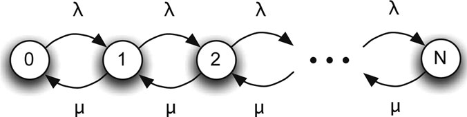
Figure 17.4:  State transition diagram for X(t).

The balance equations are now

$\begin{array}{lll}{\text{λπ}}_0\hfill & =\hfill & \mu {\text{π}}_1\hfill \\ {\text{λπ}}_1\hfill & =\hfill & \mu {\text{π}}_2\hfill \\ \hfill & :\hfill & \hfill \\ {\text{λπ}}_{N-1}\hfill & =\hfill & \mu {\text{π}}_N\hfill \end{array}$

(17.32)

with the additional constraint π₀ + π₁ + ⋯ + π_Ν = 1. The solution for the steady-state probabilities is

${\text{π}}_j=\frac{\left(1-\rho \right){\rho }^j}{1-{\rho }^{N+1}}$

(17.33)

for j = 0, 1, …, N.

If a finite sized buffer for packets is represented as an M/M/1/N queue, the probability that a packet will be lost is the same as the probability that an arrival will find the system full upon arrival:

$Pr\left(loss\right){\text{= π}}_N=\frac{\left(1-\rho \right){\rho }^N}{1-{\rho }^{N+1}}$

(17.34)

For large N, it can be seen that the probability of loss decreases exponentially with N:

$Pr\left(loss\right)\approx \left(1-\rho \right){\rho }^N$

(17.35)

For large N, one might guess that the loss probability for the M/M/1/N queue could be approximated by the tail probability for the M/M/1 queue, i.e.,

$Pr\left(loss\right)\approx P\left(X>NinM/M/1\right)$

(17.36)

This conjecture can be easily checked by comparing

$Pr\left(X>NinM/M/1\right)={\displaystyle \sum _{j=N+1}^{\infty }{\rho }^j}\left(1-\rho \right)={\rho }^{N+1}$

(17.37)

with the M/M/1/N loss probability in (17.35), which differs only by a factor of $\frac{\rho }{1-\rho }$. Thus, the M/M/1 queue may be an adequate approximation for the M/M/1/N queue for some purposes when N is very large.

17.5.1    Example: Queueing Model of a Packet Switch

The results from the performance analysis of the M/M/1/N queue are useful for analyzing the performance of the simple K × K output buffered packet switch shown in Figure 17.5. The assumptions are:

•  Poisson arrivals at rate λ at each input port;

•  packets require exponential service with rate μ at each server;

•  packets can be transferred immediately through the fabric from inputs to output buffers;

•  output buffers are finite capacity N;

•  each incoming packet is addressed to the outputs with equal likelihood, i.e., probability 1/K to any output port.

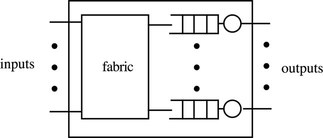
Figure 17.5:  Output buffered packet switch.

The output buffers are statistically identical so one can examine any queue. A queue receives a flow of packets from input 1 with rate λ/K, a flow from input 2 with rate λ/K, and so on. The flow from each input port is Poisson because Poisson arrivals have the property that random splitting of Poisson arrivals will maintain the Poisson character of the split processes (refer to Section 17.2.2). The queue receives the aggregate of K Poisson arrival processes, each with rate λ/K. The aggregate of independent Poisson arrivals will be Poisson. Hence, the aggregate arrivals to the queue will be Poisson with rate λ.

Since packets receive exponential service, the output queue is an M/M/1/N. It was found in (17.35) that the probability of loss for the M/M/1/N queue is approximately (1 − ρ)ρ^N. A practical problem in queueing system design is to find the necessary buffer size N for a given loss probability P_loss. By reversing (17.35), the necessary buffer capacity to meet a given loss probability is

$N=\frac{\log P_{loss}-\log \left(1-\rho \right)}{\log \rho }$

(17.38)

17.6    M/M/N/N Queue

The M/M/N/N queue is an example of a queueing system with multiple servers. The arrival process is Poisson with rate λ. Each of the N servers carries out an exponential service time with rate μ. An arrival can receive service immediately if a server is idle, or otherwise departs without service. The number in the system X_t is a truncated birth-death process with (N +1) × (N + 1) conditional rate matrix

$A=\left[\begin{array}{llllll}0\hfill & \text{λ}\hfill & 0\hfill & 0\hfill & \cdots \hfill & 0\hfill \\ \mu \hfill & 0\hfill & \text{λ}\hfill & 0\hfill & \ddots \hfill & 0\hfill \\ 0\hfill & 2\mu \hfill & 0\hfill & \text{λ}\hfill & \ddots \hfill & 0\hfill \\ ⋮\hfill & \ddots \hfill & \ddots \hfill & \ddots \hfill & \ddots \hfill & \text{λ}\hfill \\ 0\hfill & 0\hfill & \cdots \hfill & 0\hfill & N\mu \hfill & 0\hfill \end{array}\right]$

(17.39)

The balance equations are

${\text{λπ}}_{n-1}=n\mu {\text{π}}_n$

(17.40)

for n = 1, …, N with the additional constraint π₀ + ⋯ + π_Ν = 1. By substitution, the steady-state probabilities are

$\begin{array}{l}{\text{π}}_0={\left(1+\frac{\text{λ}}{\mu }+\cdots +\frac{\text{λ}}{N\mu }\right)}^{-1}\\ {\text{π}}_0=\frac{{\text{λ}}^n}{n!{\mu }^n}{\text{π}}_0,n=1,\dots ,N\end{array}$

(17.41)

The probability of losing a customer is the steady-state probability of finding the system full, π_Ν. This is the Erlang B formula applied to incoming telephone calls to a telephone switch with the capacity to support N simultaneous calls.

17.7    M/M/1 Queues in Tandem

Burke’s theorem is an important result related to the M/M/1 queue. The arrivals to an M/M/1 queue are Poisson with rate λ by definition. Burke’s theorem is surprising because it states that the departures in steady-state are Poisson as well.

Theorem 17.7.1. In steady-state, the departure process from an M/M/1 queue is a Poisson process, and the number in the queue at a time t is independent of the departure process prior to t.

At first, the result may appear to contradict intuition. By intuition, we know that the queue is either busy or free. When it is busy, packets are being served at a rate μ, so departures are separated by exponential times with mean l/μ. This implies that departures should be Poisson with rate μ. On the other hand, when the queue is free, it is waiting for the next packet arrival. The interarrival time is exponential with mean l/λ. The new arrival will be serviced immediately. Hence, its departure will be separated from the previous departure by the sum of one interarrival time and a service time. In either case, departures do not seem to be a Poisson process with rate λ.

A way to rationalize Burke’s theorem is by a time reversal argument. Recall that the number in an M/M/1 queue is a continuous-time Markov chain X_t. Specifically, it is a birth-death process with birth rates λ and death rates μ. An increment in X_t corresponds to an arrival, and a decrement in X_t corresponds to a departure. As a Markov process, it is time reversible and the time-reversed process, Y_t = X_−t is also a Markov process. It can be shown that the time-reversed process Y_t is also a birth-death process with birth rates λ and death rates μ. This implies that arrivals for Y_t are a Poisson process. But arrivals for Y_t are the same as departures for the forward-time process X_t, implying that departures from the M/M/1 queue are Poisson with rate λ.

17.7.1    Product Form

Burke’s theorem is important because it allows simple analysis of a system of multiple queues. Consider the two queues in series shown in Figure 17.6. Arrivals to the first queue are Poisson with rate λ, and both servers are exponential and independent of each other. Departures from the first queue are arrivals to the second queue. Burke’s theorem states that departures from the first queue are Poisson with rate λ, and therefore arrivals to the second queue are Poisson with rate λ. This implies that both queues are M/M/1. Both queues can be treated as independent M/M/1 queues.

Theorem 17.7.2. Let denote the joint steady-state probability that there are i in the first queue and j in the second queue. The joint steady-state probabilities can be factored into

${\text{π}}_{i,j}={\text{π}}_i^{\left(1\right)}{\text{π}}_j^{\left(2\right)}$

(17.42)

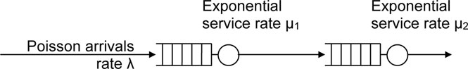
Figure 17.6:  Two queues in series.

where ${\pi }_i^{\left(1\right)}$ is the steady-state probabilities for the first M/M/1 queue, and ${\pi }_j^{\left(2\right)}$ is the steady-state probabilities for the second M/M/1 queue.

The system is said to have a product-form solution because the joint steady-state probabilities can be shown to equal the product of the steady-state probabilities for the individual queues. The product-form solution implies that the queues in series can be treated as independent M/M/1 queues.

Performance analysis is often concerned with the delay through the system (both queues). Because the queues are independent, the delay through the system equals the sum w = w₁ +w₂ where w₁ is the exponentially distributed delay through the first queue with parameter μ₁ − λ and w₂ is the exponentially distributed delay through the second queue with parameter μ₂ − λ.

17.7.2    Jackson Networks

Jackson networks have product form which conveniently allows analysis of a network of queues of any size by treating each queue as an independent M/M/1 queue. An example of an open Jackson network is shown in Figure 17.7. Jackson networks have a number of assumptions:

•  Poisson arrivals enter the network at queue i with rate λ_i;

•  customers require exponential service with rate μ_i at queue i;

•  service times at each queue are independent of other queues;

•  after service, customers are routed randomly with r_ij as the probability of going from queue i to queue j (0 denotes leaving the network).

Having product form, the Jackson network in the example can be analyzed as a network of independent M/M/1 queues. Since the service rate of each queue is given, it remains to find the aggregate arrival rate into queue i, γ_i. The aggregate rates can be found by balancing the traffic rates into and out of each queue, resulting in the system of equations:

$\begin{array}{lllll}{\text{γ}}_1\hfill & =\hfill & {\text{λ}}_{\text{1}}\hfill & +\hfill & r_{31}{\text{γ}}_3\hfill \\ {\text{γ}}_2\hfill & =\hfill & {\text{λ}}_2\hfill & +\hfill & r_{12}{\text{γ}}_1\hfill \\ {\text{γ}}_3\hfill & =\hfill & {\text{λ}}_3\hfill & +\hfill & r_{23}{\text{γ}}_2\hfill \end{array}$

(17.43)

Figure 17.7:  An open Jackson network.

These equations can be solved for the rates {γ_i} in terms of the given routing probabilities r_ij and new arrival rates λ_i.

A practical question might be the delay along a given path, for instance, through queues 1 and 2. Because the queues are independent, the delay along this path will be the sum w = w1 + w₂ where w1 is the exponentially distributed delay through the first queue with parameter μ₁ − γ_i and w₂ is the exponentially distributed delay through the second queue with parameter μ₂ − γ₂.

17.8    M/G/1 Queue

As mentioned before, the M/M/1 queue makes two assumptions that may be questionable for some applications. First, interarrival times are exponentially distributed which alleviates the need to account for the times of past arrivals. Second, service times are exponentially distributed. The memoryless property of the exponential probability distribution means it is unnecessary to account for how long the current packet has already spent in service.

In modeling packet networks, the second assumption of exponential service times is particularly questionable. The service time for a packet is the time to transmit it on a link, i.e., the ratio of its packet length to the link rate. Since transmission link rates are constant, the service times are proportional to packet lengths. The assumption of exponential service times implies that packet lengths are exponentially distributed, which is not true in actuality. Measurements of packets in the Internet have shown that the packet length distribution is not exponential. There is a wide but limited range of packet lengths, and certain packet lengths occur frequently due to the nature of protocols.

The M/G/1 queue keeps the assumption of Poisson arrivals, but allows the service times to have any given probability distribution function B(y) or probability density function b(y). The service times {y₁, y₂, …} are i.i.d. samples from B(y).

A practically important special case is the M/D/1 queue where service times are deterministic 1/μ, that is, the service time probability distribution function B(y) is a step function at y = 1/μ. The M/D/1 queue is applicable to protocols with fixed-length packets such as ATM (asynchronous transfer mode) or time-slotted data link protocols.

17.8.1    Embedded Markov Chain

Unfortunately, the number in the system X_t is no longer sufficient to represent the entire state of an M/G/1 queue, and X_t is generally not Markov. The next departure time will depend on the previous departure time because service times are not memoryless (unless B(y) is the exponential distribution). An analysis of the system needs to keep track of the number in the system X_t and the time that the current packet in service has already spent, Y_t. The bivariate process (X_t, Y_t) is Markovian but cumbersome to handle.

The analysis can be simplified to a single variable by the method of an embedded Markov chain. The idea is to carefully choose specific time instants within the X_t process that will make up a discrete-time Markov chain. After finding the steady-state probabilities for the embedded Markov chain, the steady-state probabilities can be related back to the original process X_t. Fortunately, the method of the embedded Markov chain works well for the M/G/1 queue.

Suppose the chosen embedded points are X₁, X₂, … immediately after the departure of each customer. Thus, X_n is the number of customers left behind in the system after the departure of the nth customer.

Theorem 17.8.1. X_n is a discrete-time Markov chain, and furthermore, the steady-state probabilities of X_n reflect the steady-state probabilities of the M/G/1 queue.

In other words, the steady-state probabilities of the embedded Markov chain X_n, if they can be found, will completely describe the system. It remains to explain why this result is true.

To show that X_n is Markovian, let us consider two cases. In the first case, X_n = 0 meaning that the nth packet leaves behind an empty system. The (n +1)th packet will arrive to an empty system and begin service immediately. It spends one service time within the system before leaving. Therefore, it leaves behind the number of packets that arrived during its service time. Let A_n denote the number of packets that arrive during the service time of the (n + 1)th packet. If X_n = 0, then we have established that

$X_{n+1}=A_n$

(17.44)

In the second case, suppose that X_n > 0 meaning that the nth packet leaves behind a busy system. One of the X_n waiting packets enters into service immediately and leaves after one service time. Upon the departure of the (n + 1)th packet, it leaves behind X_n − 1 of the previously waiting packets and the number of packets that arrived during its service time, A_n. Thus, if X_n > 0, we have

$X_{n+1}=X_n-1+A_n$

(17.45)

The two cases can be combined together in a single equation relating X_n+1 and Xn:

$X_{n+1}=max\left(X_n-1,0\right)+A_n$

(17.46)

This relation shows that the future X_n+1 depends directly on the current X_n, and implies that given X_n, the past {X_n−1, X_n−2, …} offers no additional information to X_n+1. The Markov property is expressed as

$Pr\left(X_{n+1}|X_n,X_{n-1},X_{n-2},\dots \right)=Pr\left(X_{n+1}|X_n\right)$

(17.47)

As a discrete-time Markov chain, X_n is defined by its transition probabilities

$p_{ij}=Pr\left(X_{n+1}=j|X_n=i\right)=\{\begin{array}{ll}{\alpha }_j\hfill & \text{if}i\text{=0}\hfill \\ {\alpha }_{j-i+1}\hfill & \text{if}i>0,j\ge i-1\hfill \\ 0\hfill & \text{otherwise}\hfill \end{array}$

(17.48)

where α_i = Pr(A_n = i) is the probability mass function for A_n. Or equivalently, X_n is defined by its transition probability matrix

$P=\left[\begin{array}{llll}{\alpha }_0\hfill & {\alpha }_1\hfill & {\alpha }_2\hfill & \cdots \hfill \\ {\alpha }_0\hfill & {\alpha }_1\hfill & {\alpha }_2\hfill & \ddots \hfill \\ 0\hfill & {\alpha }_0\hfill & {\alpha }_1\hfill & \ddots \hfill \\ ⋮\hfill & \ddots \hfill & \ddots \hfill & \ddots \hfill \end{array}\right]$

(17.49)

The next task is to find the probability mass function α_i. We note that given any service time Y, the number of arrivals during that service time will have a Poisson distribution:

$Pr\left(A_n=i|Y=y\right)=\frac{{\left(\text{λy}\right)}^i}{i!}{e}^{-\text{λ}y}$

(17.50)

The conditional probability can be unconditioned with the service time probability density function as:

${\alpha }_i=Pr\left(A_n=i\right)={\displaystyle {\int }_0^{\infty }\frac{{\left(\text{λ}y\right)}^i}{i!}{e}^{-\text{λ}y}b\left(y\right)dy}$

(17.51)

It is not possible to be more specific without a given b(y).

Given the service time probability density function b(y), we can specify the transition probabilities for X_n and then find its steady-state probabilities {π_j}. The steady-state probability π_j of the embedded Markov chain is the steady-state probability of a departure leaving behind j in the system. The next step is to relate the steady-state probabilities for the embedded Markov chain to the steady-state probabilities for the queueing system.

We will make two arguments. First, the steady-state probability of leaving behind j in the system, π_j, is the same as the steady-state probability of an arrival finding j in the system. Second, the steady-state probability of an arrival finding j in the system is the same as the steady-state probability that the system will be in state j. By these two arguments, the steady-state probabilities for the embedded Markov chain are the same as the steady-state probabilities for the queueing system.

To rationalize the first argument, consider the number in the system X_t. For a stable queue, the process goes up and down infinitely many times. The transitions when X_t jumps from j to j + 1 correspond to an arrival finding j in the system, whereas the transitions of X(t) decreasing from j + 1 to j correspond to a departure leaving behind j in the system. Over a very long time horizon, the number of transitions downward from j + 1 to j, as a fraction of all downward transitions, will be the steady-state probability that departure leaves behind j in the system, π_j. It will be the same as the number of upward transitions from j to j + 1, as a fraction of all downward transitions, which is the steady-state probability that an arrival finds j in the system.

The second argument is justified by the PASTA property of Poisson arrivals in the M/G/1 queue. By the PASTA property, the probability that Poisson arrivals will find j in the system is the same as the steady-state probability that the system will be in state j. We had just established that the steady-state probability that an arrival finds j in the system will be equal to π_j. Therefore, PASTA implies that π_j is the steady-state probability that the system will be in state j.

17.8.2    Mean Number in System

The most important result for the M/G/1 queue is the Pollaczek-Khinchin (P-K) mean-value formula which gives the mean number or mean delay for the M/G/1 queue (they are directly related through Little’s formula).

Theorem 17.8.2. The P-K mean value formula: the mean number in the M/G/1 queue is

$E\left(X\right)=\rho +\frac{{\text{λ}}^{2}E\left(Y^2\right)}{2\left(1-\rho \right)}$

(17.52)

where ρ = λ/μ and E(Y²) is the second moment of the service time Y.

Interestingly, the P-K mean-value formula says that the mean number in the M/G/1 queue depends only on the utilization factor and the second moment of the service time. It does not depend on the entire service time probability distribution function.

The P-K mean-value formula can be rewritten in different forms. For example, substituting the coefficient of variation defined as the variance normalized by the squared mean:

$C_y^2=\frac{\upsilon ar\left(Y\right)}{{\left[E\left(Y\right)\right]}^2}$

(17.53)

the P-K mean-value formula can be re-expressed as

$E\left(X\right)=\rho +{\rho }^2\frac{1+C_y^2}{2\left(1-\rho \right)}$

(17.54)

In this form, the P-K mean-value formula is explicitly dependent only on the utilization and the coefficient of variation of service times, and increases linearly with the variance of service times.

If service times have more variability, the variability will cause longer queues. It reflects a general behavior of queueing systems: more randomness in the system (in either the arrival process or service times) tends to increase queueing.

The mean number in the system E(X) is the sum of the number in service and the mean number waiting in the queue. The mean number in service is ρ, so the mean number waiting in the queue is

$L_q={\rho }^2\frac{1+C_y^2}{2\left(1-\rho \right)}$

(17.55)

One of the implications of the P-K mean-value formula is that the queue length is minimized when service times are deterministic and the coefficient of variation is zero. That is, the M/D/1 queue has the shortest queues among all types of M/G/1 queues. For the M/D/1 queue, the mean number in the system will be

$E\left(X\right)=\rho \frac{{\rho }^2}{2\left(1-\rho \right)}$

(17.56)

17.8.3    Distribution of Number in System

For the probability distribution of the number in the M/G/1 queue, the important result is the P-K transform formula, which gives the probabilities for the number in the system in terms of a probability generating function. If X is the steady-state number in the system, define the probability generating function for X as

$G_X\left(z\right)=E\left(z^X\right)$

(17.57)

which is essentially the z-transform of the probability mass function of X. We will use the service time in terms of its characteristic function

$B^{\star }\left(s\right)=E\left(e^{-sY}\right)$

(17.58)

which is the Laplace transform of the service time probability density function.

Theorem 17.8.3. The P-K transform formula: the probability generating function for X is

$G_X\left(z\right)=B^{\star }\left(\text{λ}-\text{λ}z\right)\frac{\left(1-z\right)\left(1-\rho \right)}{B^{\star }\left(\text{λ}-\text{λ}z\right)-z}$

(17.59)

If the service time characteristic function (17.58) is given, we can find the probability generating function for X directly from the P-K transform formula (17.59), but unfortunately, the formula leaves the problem of finding the inverse z-transform of G_X(z). For example, let us consider the simple M/M/1 queue. The characteristic function for the exponential service time is

$B^{\star }\left(s\right)=\frac{\mu }{s+\mu }$

(17.60)

The P-K transform formula gives the probability generating function as

$G_X\left(z\right)=\frac{1-\rho }{1-\rho z}$

(17.61)

The inverse z-transform of G_X(z) is the probability mass function for X. Fortunately, in the case of the M/M/1 queue, the inverse z-transform can be readily recognized as the geometric probabilities

$Pr\left(X=j\right)=\left(1-\rho \right){\rho }^j$

(17.62)

which agrees with our earlier results for the M/M/1 queue.

17.8.4    Mean Delay Through System

We know from Little’s formula that the mean delay W is related directly to the mean number in the system L by L = λW. Thus, another version of the P-K mean-value formula (17.52) is for the mean delay:

$W=\frac{1}{\mu }+\frac{\text{λ}E\left(Y^2\right)}{2\left(1-\rho \right)}$

(17.63)

Again, the mean delay is minimized when service times are deterministic, i.e., the M/D/1 queue. For the M/D/1 queue, the mean delay through the M/D/1 system is

$W=\frac{1}{\mu }+\frac{\text{λ}}{2\mu \left(\mu -\text{λ}\right)}$

(17.64)

17.8.5    Distribution of Delay Through System

Little’s formula states an explicit relationship between the mean number and the mean delay. A more general relationship exists between the probability distributions for the number in the system and delay through the system. From this relationship, one would expect that an equivalent version of the P-K transform formula (17.59) gives the probability distribution of the delay through the M/G/1 queue.

Theorem 17.8.4. Another version of the P-K transform formula is

$F^{\star }\left(s\right)=B^{\star }\left(s\right)\frac{s\left(1-\rho \right)}{s-\text{λ}+\text{λ}{B}^{\star }\left(s\right)}$

(17.65)

where F*(s) = E(e^−sw) is the characteristic function for the delay through the system w.

The formula leaves the problem of finding the inverse Laplace transform of F*(s) which will be the probability density function of w, say f(w).

As an example, consider the characteristic function for exponential service

$B^{\star }\left(s\right)=\frac{\mu }{s+\mu }$

(17.66)

The P-K transform formula (17.65) gives

$F^{\star }\left(s\right)=\frac{\mu -\text{λ}}{s+\mu -\text{λ}}$

(17.67)

Fortunately in this case, the inverse Laplace transform can be recognized easily as the exponential probability density function

$f\left(w\right)=\left(\mu -\text{λ}\right)e^{-\left(\mu -\text{λ}\right)w}$

(17.68)

which agrees with our earlier result for delay through the M/M/1 queue.

17.8.6    Example: Mixed Packets

Freedom from a restriction to exponential service times makes the M/G/1 queue generally more useful than the M/M/1 queue for analysis of packet networks. Consider the output buffer of a packet switch. We assume the usual Poisson arrivals, but there are three classes of packets, each requiring a different exponential service time (or in other words, each class has a different packet length distribution). The composition of traffic is listed in the table.

Class	Prob(class)	Mean service time
1	0.7	1
2	0.2	3
3	0.1	10

The first step in the analysis of an M/G/1 queue is identification of the service time distribution. In this example, the overall service time Y is a mixture of three exponential distributions:

$\begin{array}{l}B\left(y\right)=Pr\left(Y\le y|class1\right)Pr\left(class1\right)+Pr\left(Y\le y|class2\right)Pr\left(class2\right)\\ +Pr\left(Y\le y|class3\right)Pr\left(class3\right)\\ =0.7\left(1-e^{-y}\right)+0.2\left(1-e^{-y/3}\right)+0.1\left(1-e^{-y/10}\right)\end{array}$

(17.69)

Differentiating with respect to y, the service time probability density function is

$b\left(y\right)=0.7e^{-y}+\frac{0.2}{3}{e}^{-y/3}+\frac{0.1}{10}{e}^{-y/10}$

(17.70)

The P-K mean-value formula needs the first two moments of the service time. The mean service time is

$\begin{array}{l}E\left(Y\right)=0.7E\left(Y|class1\right)+0.2E\left(Y|class2\right)+0.1E\left(Y|class3\right)\\ =2.3\end{array}$

(17.71)

The second moment of the service time is

$\begin{array}{l}E\left(Y^2\right)=0.7E\left(Y^2|class1\right)+0.2E\left(Y^2|class2\right)+0.1E\left(Y^2|class3\right)\\ =25\end{array}$

(17.72)

The P-K mean-value formula (17.63) states the mean delay through the system is

$W=E\left(Y\right)+\frac{\text{λ}E\left(Y^2\right)}{2\left(1-\rho \right)}=2.3+\frac{25\text{λ}}{2\left(1-2.3\text{λ}\right)}$

(17.73)

We can continue with the P-K transform formula to find the distribution of delay through this system. The P-K transform formula (17.65) needs the service time characteristic function B*(s) which in this example can be found as

$\begin{array}{l}B*\left(s\right)=E\left(e^{-sY}|class1\right)Pr\left(class1\right)+E\left(e^{-sY}|class2\right)Pr\left(class2\right)\\ +E\left(e^{-sY}|class3\right)Pr\left(class3\right)\\ =0.7\frac{1}{s+1}+0.2\frac{1/3}{s+1/3}+0.1\frac{1/10}{s+1/10}\\ =\frac{0.7}{s+1}+\frac{0.2}{3s+1}+\frac{0.1}{10s+1}\end{array}$

(17.74)

According to the P-K transform formula, the characteristic function for the delay through the system w is

$F*\left(s\right)\left(\frac{0.7}{s+1}+\frac{0.2}{3s+1}+\frac{0.1}{10s+1}\right)\frac{s\left(1-\rho \right)}{s-\text{λ}+\text{λ}\left(\frac{0.7}{s+1}+\frac{0.2}{3s+1}+\frac{0.1}{10s+1}\right)}$

(17.75)

Unfortunately, the inverse Laplace transform of F*(s) in this example is not immediately obvious.

17.8.7    Example: Data Frame Retransmissions

For another example, suppose that a data frame is transmitted and stored in the buffer until a positive acknowledgement is received with probability p. The time from the start of frame transmission until an acknowledgement is a constant T. With probability 1 − p, the acknowledgement will be negative, necessitating a retransmission. Each retransmission is an independent Bernoulli trial with probability p of a successful transmission. After a successful transmission, the data frame can be deleted from the buffer, and the next frame waiting in the buffer will be transmitted.

With the usual assumption of Poisson packet arrivals at rate λ, the system can be modeled by an M/G/1 queue. The “effective” service time is T with probability p, 2T with probability (1 − p)p, and generally nT with probability (1 − p)ⁿ⁻¹p. For this geometric service time, the mean is

$E\left(Y\right)=\frac{T}{p}$

(17.76)

and second moment is

$E\left(Y^2\right)=\frac{T^2\left(2-p\right)\left(1-p\right)}{p^2}$

(17.77)

The P-K mean-value formula (17.63) states the mean delay through the system is

$W=\frac{T}{p}+\frac{\text{λ}{T}^2\left(2-p\right)\left(1-p\right)}{2p\left(p-\text{λ}T\right)}$

(17.78)

17.9    Conclusions

This chapter has covered basic queueing theory encompassing the simple M/M/1 queue to the intermediate M/G/1 queue. The M/M/1 queue is particularly useful because its analysis can be extended to product-form networks. The M/G/1 queue is also fairly useful for networking problems because the service time can be general and the P-K formulas allow straightforward analysis. Unfortunately, the assumption of Poisson arrivals limits the applicability of these models.

This chapter has not covered the general G/G/1 queue which can be approached by means of Lindley’s integral equation. Although general, the G/G/1 queue is quite difficult for analysis. It is often questionable whether an exact queueing analysis is worth the effort when queueing models are usually a conceptual approximation to real problems. Simpler models such as the stochastic fluid buffer have been successful alternatives to queueing models because they are more tractable, even though they appear at first to be more abstract.

Advanced queueing theory also covers a variety of complications such as service scheduling algorithms (essentially priorities), service preemption, multiple queues, and buffer management or selective discarding algorithms. The literature on queueing theory and its applications to networking problems is vast due to the many possible variations of the basic queueing models.

17.10  Exercises

Exercise 17.10.1. Consider a discrete-time Markov chain X_n with only two states, 0 and 1. The initial state is X₀ = 0. Its transition probability matrix is

$P=\left[\begin{array}{c}0.30.7\\ 0.60.4\end{array}\right]$

(17.79)

(a) Find the steady-state probabilities. (b) What are the state probabilities at time n = 3 and n = 6? Do they seem to be approaching the steady-state probabilities?

Exercise 17.10.2. Sometimes a metric called “power” is defined as the ratio of throughput to mean delay. (a) Find the power for a stable M/M/1 queue (note the throughput is the same as the arrival rate λ). (b) Find the value of ρ to maximize power.

Exercise 17.10.3. (a) For the M/M/1 queue, use the steady-state probabilities to find the mean number waiting in the queue (excluding any in service), denoted L_q. (b) Find the mean waiting time in the queue W_q as the difference between the mean delay through the system and mean service time. (c) Verify that Little’s formula holds for the queue excluding the server, i.e., L_q = λW_q.

Exercise 17.10.4. For an M/M/1 queue, find the allowable utilization factor such that 99% of customers do not experience a delay through the system more than a given T.

Exercise 17.10.5. Consider an M/M/1/2 queueing system in which each customer accepted into the system brings in a profit of $5 and each customer rejected results in a loss of $1. Find the profit for the system.

Exercise 17.10.6. Consider an output buffered packet switch where the output buffers are modeled as M/M/1/N queues. (a) With λ = 100, μ = 150, what buffer size N is required to meet a loss probability of 10⁻⁶? (b) Suppose λ and μ are both increased by a factor of 10 (representing a scaled up switching speed), how would the answer to part (a) change?

Exercise 17.10.7. Consider two M/M/1 queues in series. The first exponential server has rate μ₁ and the second has rate μ₂. (a) Under the constraint the sum of service rates is fixed to a constant, μ₁ + μ₂ = μ, find the mean delay through the system (both queues). (b) Find μ₁ and μ₂ under the constraint that their sum is fixed, to minimize the mean delay through the system.

Exercise 17.10.8. (a) Find the mean number in the M/D/1 queue as a function of ρ. (b) Find the ratio of the mean number in the M/D/1 queue to the mean number in the M/M/1 queue. Is the ratio less than one?

Exercise 17.10.9. Use the P-K transform formula for the M/D/1 queue. (a) Find the characteristic function for the delay through the system. (b) Find the characteristic function for the waiting time in the queue.

Exercise 17.10.10. Define X_n is the number of customers left behind in an M/D/1 system after the departure of the nth customer. (a) Describe the transition probabilities for this discrete-time Markov chain. (b) Set up the balance equations for the steady-state probabilities.

Exercise 17.10.11. Consider an M/G/1 queue with two classes of packets. Class 1 packets arrive as a Poisson process with rate λ₁ and require a constant service time μ₁. Class 2 packets arrive as a Poisson process with rate λ₂ and require a constant service time μ₂. Find the mean delay through the system.

References

[1]  Bolch, G., Greiner, S., de Meer, H., and Trivedi, K. S., Queueing Networks and Markov Chains: Modeling and Performance Evaluation with Computer Science Applications, Wiley Interscience, Hoboken, NJ, 2006.

[2]  Bose, S., An Introduction to Queueing Theory, Springer, New York, 2001.

[3]  Burke, P. J., “The output of a queuing system,” Operations Research, vol. 4, pp. 699–704, December 1956.

[4]  Daigle, J., Queueing Theory with Applications to Packet Telecommunication, Springer, New York, 2010.

[5]  Gelenbe, E., and Pujolle, G., Introduction to Queueing Networks, Wiley, Chichester, UK, 1998.

[6]  Gross, D., Shortle, J., Thompson, J., and Harris, C., Fundamentals of Queueing Theory, 4th ed., Wiley Interscience, Hoboken, NJ, 2008.

[7]  Jackson, J. R., “Jobshop-like queueing systems,” Management Science, vol. 10, pp. 131–142, 1963.

[8]  Kleinrock, L., Queueing Systems Volume 1: Theory, Wiley Interscience, New York, 1975.

[9]  Little, J. D. C., “A proof of the queueing formula L = λW,” Operations Research, vol. 9, pp. 383–387, 1961.

[10]  Medhi, J., Stochastic Models in Queueing Theory, 2nd ed., Academic Press, San Diego, 2002.

[11]  Robertazzi, T., Computer Networks and Systems, 3rd ed., Springer, New York, 2000.

[12]  Wolff, R., Stochastic Modeling and the Theory of Queues, Prentice Hall, Englewood Cliffs, NJ, 1989.