Chapter 15  Linear Programming and Mixed Integer Programming

Bogdan Dumitrescu^‡

‡ Tampere University of Technology, Finland

Linear programming (LP) is the class of optimization problems whose criterion and constraints are linear. Such problems appeared first in economy, for example in activity planning or resource allocation, but are now ubiquitous also in engineering. Although being apparently the simplest type of optimization problem that has no analytic solution, LP has interesting properties and its study has led to significant developments and generalizations for the whole optimization field, both in terms of theory and algorithms.

Mixed integer programming (MIP) problems also have linear criterion and constraints, but some of their variables are constrained to integer values. Despite their resemblance to LP, they have distinct properties and are solved by dedicated algorithms, using LP as a fundamental tool, but much more complex.

This chapter will present the basic theory, the main algorithmic approaches and a few typical signal processing problems that can be modeled through LP or MIP.

15.1    Linear Programming

Having linear criterion and constraints, LP belongs to convex optimization and shares all the good properties given by convexity. Some of these properties have particular forms that can be used for designing algorithms tailored specifically for LP. Besides an introduction to the standard LP forms and transformations that lead to them, this section contains characterizations of optimality and, in particular, duality, and a short presentation of the two main algorithmic solutions to LP: the simplex method and interior-point methods.

15.1.1    General Presentation

An LP problem, in standard (named also primal, or equality) form, is

$\begin{array}{ll}\mu =\min \hfill & c^{T}x\hfill \\ \hspace{0.17em}\hspace{0.17em}\hspace{0.17em}\hspace{0.17em}\hspace{0.17em}\hspace{0.17em}\hspace{0.17em}\hspace{0.17em}\hspace{0.17em}\hspace{0.17em}\hspace{0.17em}\hspace{0.17em}\mathrm{s.t}.\hfill & Ax=b\hfill \\ \hfill & x\ge 0\hfill \end{array}$

(15.1)

By x ≥ 0 we understand that each element of the vector x ∈ ℝⁿ is non-negative. We name μ the value of the LP problem; we denote x* a solution of the problem, i.e., a vector for which c^Tx* = μ, Ax* = b, x* ≥ 0. The matrix A has m rows and n columns. Typically, the number of rows is smaller, otherwise it may easily happen that the system Ax = b has no solution at all. We assume that A has independent rows, i.e., rank (A) = m; if this is not the case, the redundant rows of A can be eliminated using the QR factorization before solving the LP problem. Even with these assumptions, Problem (15.1) may be infeasible, when no solution of Ax = b satisfies the positivity constraint; in this case we conventionally put μ = ∞. Due to the linearity of the constraints, the feasible domain is a polytope that may be bounded or unbounded. Since the gradient of the criterion is c and hence constant, if (15.1) has a finite solution, then it lies on the boundary of the feasible polytope, i.e., it is a vertex, an edge or even an entire face. If the polytope is unbounded in the direction —c, then the criterion can decrease indefinitely; the LP problem is unbounded and μ = −∞.

Example 15.1.1. The LP problem

$\begin{array}{ll}\min \hfill & x_2+x_3\hfill \\ \mathrm{s.t}.\hfill & 0.8x_1+0\mathrm{.5}{x}_2+x_3=1\hfill \\ \hfill & x_1\ge 0,x_2\ge 0,x_3\ge 0\hfill \end{array}$

(15.2)

is a particular case of (15.1), with A = [0.8 0.5 1], b =1, c =[0 1 1]^T. Its feasible domain is the gray triangle shown on the left of Figure 15.1. The criterion decreases along the direction −c = [0 − 1 − 1]^T and so the optimum is attained when x₂ and x₃ have their least possible values; the solution is x* = [1.25 0 0]^T, a vertex of the feasible triangle.

All types of linear constraints can be brought to the standard form (15.1). An inequality Ax ≤ b can be transformed into the equality Ax + s = b, by adding a vector s ≥ 0 of slack variables. Similarly, the inequality Ax ≥ b is transformed into Ax − s = b, now s ≥ 0 being named surplus. Finally, if the variable x is unrestricted, it can be expressed as x = x+ − x₋, with x₊ ≥ 0, x₋ ≥ 0; if x can have negative values but it has a lower bound x ≥ x₀, then x is substituted with x − x₀ ≥ 0, which changes the equality constraint of (15.1) into Ax = b + Ax₀. Concerning the criterion, if the LP problem would imply maximization of c^Tx, then this is equivalent to minimizing −c^Tx, i.e., the sign of the vector c is changed for getting the standard form. Note that several of the above transformations increase the number of variables when bringing the problem to standard form; however, the standard form has the advantage of efficient specialized algorithms.

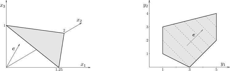
Figure 15.1:  Feasible domains of the LP problems from Examples 15.1.1 (left) and 15.1.2 (right).

Another common formulation of LP problems is in the inequality (named also dual) form

$\begin{array}{ll}\max \hfill & e^{T}y\hfill \\ \mathrm{s}.\mathrm{t}.\hfill & Dy\le f\hfill \\ \hfill & \hfill \end{array}$

(15.3)

The variable y ∈ ℝ^m is unrestricted and the constraints are only in inequality form, with all variables at the left of the “≤” sign and the free term at the right. Typically, the matrix D ∈ ℝ^n×m has more rows than columns. Again, one can bring any LP problem to form (15.3), if so desired. The inequality Dy ≥ f is transformed by reversing the sign into −Dy ≤ −f. Equality constraints are transformed by variable elimination. Consider a single equality g^Ty = α; the vector g has at least a non-zero component, say, g_k; it results that y_k = (α − ∑_i≠k g_iy_i) /g_k; this expression of y_k is substituted in all the other constraints of the optimization problem and hence the variable y_k is eliminated.

Example 15.1.2. The LP problem

$\begin{array}{rrrrrr}\hfill \max & \hfill y_1& \hfill +& \hfill y_2& \hfill & \hfill \\ \hfill \mathrm{s}.\mathrm{t}.& \hfill -y_1& \hfill & \hfill & \hfill \le & \hfill -1\\ \hfill & \hfill y_1& \hfill & \hfill & \hfill \le & \hfill 5\\ \hfill & \hfill -y_1& \hfill -& \hfill 2y_2& \hfill \le & \hfill -3\\ \hfill & \hfill y_1& \hfill -& \hfill y_2& \hfill \le & \hfill 3\\ \hfill & \hfill -y_1& \hfill +& \hfill 4y_2& \hfill \le & \hfill 11\end{array}$

(15.4)

is a particular case of (15.3). Its feasible domain is the gray polygon shown on the right of Figure 15.1; the reader is invited to identify the correspondence between the five edges of the polygon and the five inequality constraints. The level curves are lines for which y₁ + y₂ is constant and are drawn with dashed lines; they are orthogonal to the gradient e = [1 1]^T. The criterion increases along the direction of the gradient. The optimum is attained in y* = [5 4]^T, again a vertex of the feasible polygon. If the criterion were defined by e = [1 0]^T, then the solution would be the whole rightmost edge of the polygon, defined by y₁ =5 and 2 ≤ y₂ ≤ 4. Finally, if the last constraint would be removed, the upper edge of the polygon would disappear; the polygon would become unbounded and the value y₁ + y₂ would grow indefinitely since y₂ has no upper bound; the LP problem would be unbounded.

15.1.2    Transformations of the Standard Problem

The data of Problem (15.1), namely A, b and c, can be transformed such that an equivalent problem is obtained (in the sense that the transformed problem has the same solution as (15.1)), also in standard form. Here we denote the data of the transformed problem by Ã, b̃ and c̃, but in general the transformations are performed in place. The two important transformations are the following:

(i) Reordering the variables: x̃ = Px, where P ∈ ℝ^n×n is a permutation matrix. Since Ax = AP^TPx, this is equivalent to the transformation à = AP^T, c̃ = Pc, which amounts to rearrange the columns of A and the elements of c according to the permutation of the variable. The vector b is unchanged. We will often assume that the variables are conveniently ordered, since this does not change the values of the solution.

(ii) Multiplication with a nonsingular matrix M ∈ ℝ^m×m at the left: since MAx = Mb has the same solution as Ax = b, the transformation à = MA, b̃ = Mb is valid. The vector c is not affected. In particular, M can be a permutation matrix, in which case the transformation consists of permuting the equations of the system Ax = b.

An example of transformed problem is the canonical form, in which (we will describe all transformations as performed in place)

$\tilde{A}\to A=\left[\begin{array}{lllllll}1\hfill & 0\hfill & \dots \hfill & 0\hfill & a_{1,m+1}\hfill & \dots \hfill & a_{1,n}\hfill \\ 0\hfill & 1\hfill & \dots \hfill & 0\hfill & a_{2,m+1}\hfill & \dots \hfill & a_{2,n}\hfill \\ \hfill & \hfill & ⋮\hfill & \hfill & \hfill & ⋮\hfill & \hfill \\ 0\hfill & 0\hfill & \dots \hfill & 1\hfill & a_{m,m+1}\hfill & \dots \hfill & a_{m,n}\hfill \end{array}\right].$

(15.5)

We assume that the first columns of A are linearly independent; if this is not the case, permutation of columns can be used. The above form can be obtained via Gauss-Jordan elimination. The process has m steps and, in step i, column i of A is transformed into the i-th unit vector e_i (whose elements are zero, excepting the i-th, which is equal to 1). To this purpose, we first divide equation i of Ax = b by a_i,i, which means that the i-th row of A and b_i are divided by a_i,i. (If a_i,i = 0, then pivoting is necessary: equation i of Ax = b is permuted with equation k > i, for which a_k,i ≠ 0. A better numerical choice is to always pivot, using the largest |a_k,i|. Also, complete pivoting can be used, searching the largest |a_k,ℓ|, with k ≥ i, ℓ ≥ i; a column permutation, i.e., transformation of type (i) may be necessary.) Then, we apply of transformation of type (ii), with

$\begin{array}{cc}{M}_i=I-m_i{e}_i^T,& \mathrm{with}{m}_i\end{array}={\left[a_{1,i}\dots a_{i-1,i}0a_{i+1,i}\dots a_{i+m}\right]}^T.$

These operations amount to multiply equation i of Ax = b with a_k,i and subtract it from equation k, for each k ≠ i. Note that the first i − 1 columns of A are not affected, since the i-th row of A has zeros in its first i − 1 positions.

Complete pivoting has the advantage that it always finds m independent columns if rank (A) = m; if the rank is smaller, then the last m – rank (A) rows of the transformed matrix are zero and hence can be eliminated or, if the corresponding elements of b are non-zero, infeasibility is detected. However, orthogonal transformations are numerically better to detect rank deficiency.

The canonical form (15.5) is used in the implementation of the simplex method, discussed in Section 15.1.5.

15.1.3    Optimality Characterization

We look now at the LP standard form (15.1) and present some properties related to optimality. The next result is the most significant.

Theorem 15.1.3. If the LP problem (15.1) has finite value, then it has a solution x* with at most m non-zero elements.

Proof. If (15.1) has finite value, then the optimum is attained. Assume that x is a solution of (15.1) having the minimum number p > m of non-zero elements. Without loss of generality, we can assume that these are x₁, x₂, …, x_p. Since rank (A) < p, it results that the first p columns of A are linearly dependent and so there exists a vector u ≠ 0, with u_i = 0 for i > p, such that Au = 0. We can assume that c^Tu ≥ 0, otherwise we take − u instead of u.

Suppose first that c^Tu ≥ 0. Since x_i ≥ 0 for i = 1: p, it results that for some ε > 0 small enough, it is true that x_i − εu_i ≥ 0. Putting, x̃ = x − εu, it results that Ax̃ = b, x̃ ≥ 0 and c^Tx̃ < c^Tx. Hence, x is not optimal.

Suppose now that c^Tu = 0. Since u ≠ 0, we can vary ε (no longer constrained to be positive) until one of the first p components of x̃ = x − εu becomes zero, the others remaining positive. It results that x̃ is also a solution of (15.1), but has p − 1 non-zero elements.

Hence the assumption p > m leads to a contradiction, and so the theorem is proved.

■

Let $\mathcal{I}$ be a subset of 1 : n having m elements. If x satisfies the constraints of (15.1), the elements x_i are zero for i ∉ $\mathcal{I}$ and the matrix B formed by the columns of A with indices in $\mathcal{I}$ is nonsingular, then x is named a basic feasible point. If x_i > 0, ∀i ∈ $\mathcal{I}$, then the basic feasible point is called nondegenerate. The set of variables x_i with i ∈ $\mathcal{I}$ is called a base (equivalently, $ℐ$ may be called the base).

Theorem 15.1.4. A vector x is a basic feasible point if and only if it is a vertex of the feasible polytope of the LP problem (15.1).

Proof. Assume that x is a basic feasible point and that there exist feasible vectors v and w, both different from x, and λ ∈ (0, 1) such that x = λν +(1 − λ)w, i.e., x is not a vertex of the feasible polytope. Let v₁ = [υ_i]_i∈$ℐ$, v₂ = [v_i]_i∉$ℐ$; define similarly w₁, w₂, x₁, x₂ and note that x₂ = 0. Since λν₂ + (1 − λ)w₂ = x₂ =0, v₂ ≥ 0, w₂ ≥ 0 (v and w are feasible) and λ > 0, 1 − λ > 0, it results that v₂ = w₂ = 0. It follows that Av = Bv₁ = b, Aw = Bw₁ = b and so Bv₁ = Bw₁. Since B is nonsingular, we conclude that v₁ = w₁, which is impossible since it would imply that v = w = x, contrary to the initial assumptions. So, x must be a vertex.

Conversely, assume that x is a vertex and has p non-zero elements. Define $\mathcal{I}$ = {i ∈ 1 : n | x_i ≠ 0}. Let B = [a_i]_{i∈$\mathcal{I}$}, i.e., the submatrix of A made of the columns corresponding to the non-zero elements of x. Assume that rank(B) < p, i.e., the columns of B are not linearly independent. Then, as in the proof of Theorem 15.1.3, there exists u ≠ 0, with u_i = 0 for i ∉ $\mathcal{I}$, such that Au = 0. Then, for ε small enough, v = x + ℰu and w = x − ℰu are both feasible and x = (v + w) /2, hence x is not a vertex. This contradicts our hypothesis on the rank of B. It results then that rank(B) = p ≤ m (if p > m, the columns of B cannot be linearly independent). If p = m, then x is a basic feasible point. If p < m, since rank (A) = m, there are m − p columns of A that added to those of B make a nonsingular matrix, hence fulfilling the conditions for a basic feasible point.

■

Corollary 15.1.5. If the LP problem (15.1) has finite value, then it has a solution that is a basic feasible point.

Proof. Theorem 15.1.3 says that there exists a solution x with p ≤ m nonzero elements and its proof shows that the corresponding p columns of A have maximum rank (otherwise we can decrease p, like in the proof). The end of the proof of Theorem 15.1.4 shows that in this case x is a basic feasible point.

■

So, we have proved rigorously that, as suggested by simple geometric analysis, a vertex of the feasible polytope is always a solution of the LP problem (15.1) (this does not exclude the existence of other solutions that are not vertices). This property and the notion of basic feasible point are essential in the understanding of the simplex method.

15.1.4    Duality Aspects

The Lagrangian associated with the LP standard problem (15.1) is

$L\left(x,y,s\right)=c^{T}x+y^T\left(b-Ax\right)-s^{T}x,$

(15.6)

where y ∈ ℝ^m is the vector of Lagrange multipliers associated with the equality constraints and s ∈ ℝⁿ, s ≥ 0, the vector of multipliers associated with the inequality x ≥ 0. The Lagrange dual of the optimization problem (15.1) is

$\underset{y,s}{\max }\underset{x}{\hspace{0.17em}\inf }\hspace{0.17em}L\left(x,y,s\right).$

(15.7)

The Lagrangian L(x, y, s) = (c − A^Ty − s)^Tx + y^Tb is linear in x, so it is unbounded from below when the term multiplying x is non-zero, hence producing

$\underset{x}{\inf }L\left(x,y,s\right)=\{\begin{array}{ll}{b}^{T}y,\hfill & \text{if}{A}^{T}y+s=c\hfill \\ -\infty \hfill & \text{otherwise}\hfill \end{array}$

(15.8)

Taking into account that s ≥ 0, it results that the dual of (15.1) is

$\begin{array}{ll}\mathcal{V}=\max \hfill & b^{T}y\hfill \\ \mathrm{s}.\mathrm{t}.\hfill & A^{T}y\le c\hfill \end{array}$

(15.9)

This is an LP problem in inequality form (15.3), with D = A^T, e = b, f = c; this justifies the name dual associated with (15.3). Conversely, the dual of (15.3) is an LP problem in standard form (15.1), see Exercise 15.4.

Since LP is a convex optimization problem, strong duality holds, i.e., the primal and dual problems have the same optimal value. For LP, unlike for other convex problems, no special assumption (like the Slater condition) is required for strong duality: feasibility is enough.

Theorem 15.1.6. If one of the problems (15.1) and (15.9) is feasible, then their optimal values are equal, namely: (a) if one of the problems has finite value, then the other has the same value, i.e., μ = ν, c^Tx* = b^Ty*, where x* and y* are solutions of (15.1) and (15.9), respectively; (b) if one of the problems is unbounded, then the other is infeasible.

Proof. Since inf_x L(x, y, s) ≤ c^Tx*, the construction (15.7) of the dual problem implies that b^Ty ≤ c^Tx for any feasible x, y, i.e., ν ≤ μ. So, if the primal is unbounded (μ = − ∞), then the dual is infeasible; if the dual is unbounded (ν = ∞), then the primal is infeasible. We will prove that if the primal has finite value, then the dual has the same value; the reverse implication can be proved similarly. We present two proofs. The first is simple, but treats only the typical case when x^* is a nondegenerate basic feasible point; hence, the proof is incomplete. The second is general, but more technical; for brevity, we use Farkas’ lemma.

Proof 1. Corollary 15.1.5 says that x* is a basic feasible point. Assume, without loss of generality, that the first m variables form the base and A = [BN], with B ∈ ℝ^{m × m} nonsingular. Split $x^T=\left[x_1^T{x}_2^T\right]$, $c^T=\left[c_1^T{c}_2^T\right]$, where the first component has length m. Since $x_2^{\star }=0$, it results that $x_1^{\star }=B^{-1}b$ and $\mu =c^T{x}^{\star }=c_1^T{B}^{-1}b$. For any feasible x, it follows from Ax = b that

$B{x}_1+N{x}_2=b\Rightarrow x_1=B^{-1}\left(b-N{x}_2\right)=x_1^{\ast }-B^{-1}N{x}_2$

(15.10)

and so

${\mathrm{c}}^T\mathbf{x}+{\mathrm{c}}_1^T{\mathbf{x}}_1+{\mathrm{c}}_1^T{\mathbf{x}}_2={\mathrm{c}}_1^T{\mathrm{B}}^{-1}\mathrm{b}+\left({\mathrm{c}}_2^T-{\mathrm{c}}_1^T{\mathrm{B}}^{-1}\mathrm{N}\right){\mathbf{x}}_2=\mu +{\mathrm{r}}^T{\mathbf{x}}_2,$

(15.11)

where we have denoted r = c₂ − N^TB^−Tc₁. Assume now that x* is nondegenerate, i.e., $x_1^{\star }>0$ (remind that this assumption makes the proof incomplete). Suppose that the vector r has at least one negative element. Then, there exists x₂ ≥ 0 such that r^Tx₂ ≤ 0. Since ‖x₂‖ can be taken arbitrarily small, it results that x₁ given by (15.10) can stay into any neighborhood of $x_1^{\star }$, such that x₁ ≥ 0. Summing up, for such an x₂, we have obtained x ≥ 0 such that Ax = b and c^Tx < μ, which contradicts the optimality of x^*. So, the inequality r ≥ 0 must hold.

The constraint of the dual (15.9) has the form

$\left[\begin{array}{c}{\mathbf{B}}^T\\ {\mathbf{N}}^T\end{array}\right]y\le \left[\begin{array}{c}{\mathbf{c}}_1\\ {\mathbf{c}}_2\end{array}\right].$

We build y* by forcing the first m inequality constraints to be active, i.e., to become equalities, which implies that y* = B^Tc₁. It results that

${\mathbf{b}}^T{\mathbf{y}}^{\ast }={\mathbf{b}}^{\mathbf{T}}{\mathbf{B}}^{-T}{\mathrm{c}}_1={\mathrm{c}}_1^T{\mathbf{x}}_1^{\ast }=\mu$

and

$\mathrm{r}\ge 0\Rightarrow {\mathbf{N}}^T{\mathbf{B}}^{-T}{\mathrm{c}}_1\le {\mathrm{c}}_2\Rightarrow {\mathbf{N}}^T{\mathbf{y}}^{\ast }\le {\mathrm{c}}_2,$

so y* is feasible and optimal.

Proof 2. Given a matrix Φ ∈ ℝ^p×q and a vector f ∈ ℝ^p, the celebrated Farkas lemma says that exactly one of the following affirmations holds (this type of result is often named a “theorem of alternatives”).

 (i)  ∃u ∈ c such that Φu = f and u ≥ 0.

(ii)  ∃v ∈ ℝ^p such that Φ^Tv ≥ 0 and f^Tv ≤ 0.

The proof of Farkas’ lemma is based on the construction of a hyperplane that separates two convex sets and we omit it. However, a geometric interpretation is very intuitive. If (i) holds, then f lies in the cone formed by positive combinations of the columns of Φ. Then, a vector v cannot make simultaneously an acute angle with all columns of Φ (i.e., Φ^Tv ≥ 0) and an obtuse angle with f (i.e., f^Tv ≤ 0).

Given an arbitrary ε > 0, it results from the optimality of the primal that there is no x such that Ax = b, x ≥ 0, c^Tx = μ − ε − α, with α ≥ 0. So, there is no u = [x^T α]^T such that

$\begin{array}{cc}\left[\begin{array}{cc}A& 0\\ c^T& 1\end{array}\right]u=\left[\begin{array}{c}b\\ \mu -\epsilon \end{array}\right],& u\ge 0.\end{array}$

Hence the second alternative of Farkas’ lemma holds: there exists some v such that

$\begin{array}{cc}\left[\begin{array}{cc}{A}^T& c\\ 0& 1\end{array}\right]v\ge 0,& \left[b^T\mu -\epsilon \right]v<0.\end{array}$

Putting v = [—w^T β], it results from the above that

$-A^{T}w+\beta c\ge 0$

(15.12a)

$\beta \ge 0$

(15.12b)

$-{\mathbf{b}}^T\mathbf{w}+\beta \left(\mu -\epsilon \right)<0$

(15.12c)

If β = 0, then (15.12a) gives A^Tw ≤ 0; multiplying this inequality to the left with x^T, where x is a feasible variable, gives b^Tw ≤ 0; this contradicts (15.12c), which is b^Tw ≥ 0. Hence β ≥ 0. Putting y* = w/β, it results from (15.12a) that A^T y* ≤ c, hence y* is dual feasible, and from (15.12c) that b^Ty* > μ − ε. Since this is true for any ε − 0, it follows that b^Ty* ≥ μ. Since the dual value cannot be large than μ, we conclude that b^Ty* = μ and so the primal and dual LP problems have the same value.

■

Note that Theorem 15.1.6 does not exclude the possibility that both the primal (15.1) and dual (15.9) are infeasible; see Exercise 15.3 for an example.

The KKT optimality conditions associated with the primal (15.1) and the dual (15.9) have the form

$\mathbf{Ax}=\mathbf{b}$

(15.13a)

${\mathbf{A}}^T\mathbf{y}+\mathbf{s}=c$

(15.13b)

$\mathbf{x}\ge 0$

(15.13c)

$\mathbf{s}\ge 0$

(15.13d)

${\mathbf{s}}^T\mathbf{x}=0$

(15.13e)

The first four conditions are simply the constraints of the primal and dual problems, with the multiplier s considered. Condition (15.13e) is called complementarity slackness; since all the products s_ix_i are non-negative, this condition can be also expressed as: for all i = 1 : n, at least one of the equalities x_i =0, s_i = 0 holds. Otherwise said, an inequality constraint of (15.1) is active (x_i = 0) or the corresponding Lagrange multiplier is zero (s_i = 0), which means that the i-th inequality of the constraint A^Ty ≤ c is active in the dual (15.9). In the nondegenerate case, there are m non-zero elements in x*, see Theorem 15.1.3 and the subsequent discussion, so it results that (at least) m constraints of the dual problem must be active; typically, exactly one of $x_i^{\star }$ and $s_i^{\star }$ is zero. Note that Proof 1 of Theorem 15.1.6 actually enforces complementarity slackness.

Theorem 15.1.7. Conditions (15.13a)–(15.13e) hold if and only if both LP problems (15.1) and (15.9) are feasible and x and y are optimal.

Proof. Conditions (15.13a)–(15.13d) are equivalent to the feasibility of both the primal and the dual LP problems. By transposing (15.13a) and multiplying at the right with y, we obtain b^Ty = x^TA^Ty. By transposing (15.13b), multiplying at the right with x and making use of the previous equality, we end up with

$b^T\mathbf{y}+s^T\mathbf{x}={\mathbf{c}}^T\mathbf{x}.$

Since s^Tx ≥ 0 and b^Ty = c^Tx holds only at optimality, it results that (15.13e) is equivalent to optimality.

■

15.1.5    The Simplex Method

The simplex method, invented by Dantzig in 1947, is the first efficient algorithm for finding the solution of the LP primal problem (15.1). It is an iterative method that builds a path of vertices of the feasible polytope. At each step, it finds a vertex which shares an edge with the current vertex, such that the criterion becomes smaller. When this is no longer possible, the minimum has been attained. We present here only the main ideas of the algorithm. For a quick illustration, let us ignore that the polygon from Figure 15.1 (right) comes from a dual problem and assume that we start the search of the optimum from the point (1, 1), which is a vertex of the feasible domain. There are two paths to the optimum, hopping from a vertex to one of its better neighbors: (1, 1) → (1, 3) → (5, 4) and (1, 1) → (3, 0) → (5, 2) → (5, 4). In general, there are many such paths, one of them being followed by the simplex method.

Returning to the general case of the LP primal problem (15.1), assume that we have a basic feasible point x, which is a vertex of the feasible polytope, as affirmed by Theorem 15.1.4; finding such a point is not trivial and will be discussed later. We can transform the matrix A into the canonical form (15.5), permuting first the m variables defining the basic feasible point into the first m positions of x, then pursuing Gauss-Jordan elimination as described in Section 15.1.2. The Gauss-Jordan elimination process with row pivoting is guaranteed to succeed, i.e., to find non-zero diagonal elements, since the m columns of A defining the basic feasible point are linearly independent. We assume that all transformations have been done in place.

Note that, since x is a basic feasible point and so x_i = 0, i > m, due to the form (15.5) of the matrix A it results that x_i = b_i, i ≤ m, and hence the value of the criterion is

$z={\mathbf{c}}^T\mathbf{x}={\displaystyle \sum _{i=1}^m{b}_i{c}_i}.$

(15.14)

Since x is feasible, it necessarily results that b_i ≥ 0 at this stage.

We present now a step of the simplex method. Traveling along an edge of the feasible polytope to a neighbor vertex is equivalent to replacing a basic variable x_k, k ≤ m, with a non-basic variable x_ℓ, ℓ > m, such that a new basic feasible point is obtained and the criterion decreases; this operation is also called pivoting (not to be confused with pivoting in the elimination process described above). The set of first m variables is the base, x_k is named leaving variable, and x_ℓ entering variable. In what follows, the notations for the new basic feasible point are distinguished by a tilde. The new solution has x̃_k = 0, x̃_j = 0 for j > m, j ≠ ℓ, so equation i ≠ k of the system Ax̃ = b reads x̃_i + a_i,ℓx̃_ℓ = b_i, while equation k is simply a_k,ℓx̃_ℓ = b_k. Hence, the non-zero elements of the new solution can be found by substitution and are

$\begin{array}{l}{\tilde{x}}_{\mathit{\ell }}=\frac{b_k}{a_{k,l}},\\ \begin{array}{cc}{\tilde{x}}_i=b_i-a_{i,\mathit{\ell }}\frac{b_k}{a_{k,\mathit{\ell }}},& i=1:m.\end{array}\end{array}$

(15.15)

Note that we can obtain x̃_ℓ ≥ 0 only if a_k,ℓ > 0. Also, remark that for i = k the above formula gives the correct result x̃_k = 0.

Improvement. The entering variable x_ℓ is chosen first, such that the criterion is decreased. The value of the criterion for the new solution (15.15) is

$\tilde{z}={\mathbf{c}}^T\tilde{x}={\displaystyle \sum _{i=1}^m{c}_i}\left(b_i-a_{i,\mathit{\ell }}\frac{b_k}{a_{k,\mathit{\ell }}}\right)+c_{\mathit{\ell }}\frac{b_k}{a_{k,l}}=z+\left(c_{\mathit{\ell }}-{\displaystyle \sum _{i=1}^m{c}_i{a}_{i,\mathit{\ell }}}\right)\frac{b_k}{a_{k,\mathit{\ell }}}\underset{\_}{\underset{\_}{\mathrm{def}}}\hspace{0.17em}z+s_{\mathit{\ell }}\frac{b_k}{a_{k,\mathit{\ell }}}.$

(15.16)

The vector s whose ℓ-th element is defined in the rightmost equality is named reduced, cost and is

$\mathbf{s}=\mathbf{c}-{\mathbf{A}}^T{\left[c_1{c}_2\cdots c_m\right]}^T.$

(15.17)

Note that its first m elements are equal to zero, due to the form (15.5) of A. Moreover, once ℓ has been chosen, the vector s can be obtained in the Gauss-Jordan elimination process as if c would be appended to A as the m + 1-th row; this is how the simplex method is actually implemented.

It results from (15.16) that the criterion decreases if and only if there exists an index ℓ such that s_ℓ ≤ 0. We also conclude that, if s_i ≥ 0, for all i > m, then the optimum has been attained: no feasible direction of decrease exists. In the standard simplex method, the new variable is chosen such that s_ℓ = min{s_i | i = m +1 : n}; this is the greedy choice that hopes, but is not guaranteed, to maximize descent.

Feasibility. The leaving variable x_k is chosen such that the new solution (15.15) is feasible, namely x̃ ≥ 0. Since b_k ≥ 0 and a_k,ℓ > 0, we have to care about the sign of x̃_i only if a_i,ℓ is positive. By choosing k such that

$\frac{b_k}{a_{k,\mathit{\ell }}}=\underset{i}{min}\left\{\frac{b_i}{a_{i,\mathit{\ell }}}|a_{i,\mathit{\ell }}>0,i=1:m\right\},$

(15.18)

feasibility is ensured. Indeed, if x̃_i < 0 for some i with a_i,ℓ > 0, then

${\tilde{x}}_i\stackrel{\left(15.15\right)}{=}{b}_i-a_{i,\mathit{\ell }}\frac{b_k}{a_{k,\mathit{\ell }}}<0\Rightarrow \frac{b_i}{a_{i,\mathit{\ell }}}<\frac{b_k}{a_{k,\mathit{\ell }}},$

which contradicts the choice (15.18).

Unboundedness. A distinct possibility is that a_i,ℓ ≤ 0, for all i = 1 : m. In this case, by appending x_ℓ to the basis (hence allowing m +1 variables to be positive) and giving it an arbitrary positive value ξ, feasibility is preserved for the new solution x̃_i = b_i − a_i,ℓξ, i = 1 : m, no matter how large is ξ. Since the criterion is linear in ξ and decreases as ξ increases, the criterion goes to −∞ as ξ tends to ∞. So, in such a case, the problem is unbounded.

A sketch of the simplex method is presented in Table 15.1. Only step 3 needs further comments. After permuting columns k and ℓ of A (and c^T), only column k is not in canonical form. Since a_k,k (former a_k,ℓ) is non-zero, it can be used as a pivot to zero all the other elements of the column in a single Gauss-Jordan step, see again the paragraph after (15.5). The reduced cost is updated similarly, as if being the m + 1-th row of A.

Table 15.1:  Basic form of the simplex method.

Input data: A, b, c of the LP primal (15.1). Initialization. Find a basic feasible point. Transform A to the canonical form (15.5) by Gauss-Jordan elimination (and update b, c accordingly). Compute the reduced costs s as in (15.17). Step 1. Find entering variable index ℓ such that sℓ = min{si | i = m+1 : n}. If sℓ ≥ 0, then the optimum has been attained and the values of the base variables are xi = bi, i = 1 : m. Stop. Step 2. If ai,ℓ ≤ 0, ∀i = 1 : m, then the problem is unbounded; stop. Otherwise, find the leaving variable index k according to (15.18). Step 3. Interchange variables k and ℓ (i.e., the columns of A and the elements of c). Restore A to canonical form (15.5) and update the reduced costs. Go to step 1.

Initialization. Unless some a priori information is available, the initial basic feasible point can be found by solving, with the simplex method, the auxiliary problem

$\begin{array}{lll}\min \hfill & 1^{\mathbf{T}}\mathbf{w}\hfill & \hfill \\ \text{s}\mathrm{.t}.\hfill & \mathbf{Ax}+\mathbf{Dw}=\mathbf{b}\hfill & \hfill \\ \hfill & \mathbf{x}\ge 0,\mathbf{w}\ge 0\hfill & \hfill \end{array}$

(15.19)

where 1 = [11 … 1]^T and D = diag(b₁, b₂, …, b_m). A basic feasible point for this problem is x = 0, w = 1, so the simplex method for solving it can be initialized. Since 1^Tw ≥ 0, ∀w ≥ 0, if there exists a feasible x for the original problem (15.1), then the optimal value of problem (15.19) is zero, for w = 0, and the simplex method will find it. If the final base contains only variables from x, then it can be used as initialization for solving (15.1). However, it may happen that some variables from w are still in the base; in this case, some small alterations of the simplex method solve (15.1) with these extra variables added, but constrained to zero.

Termination. In principle, since the criterion decreases at each iteration, the path built by the simplex method does not contain loops—a vertex may appear only once. Since the number of vertices of the feasible polytope is finite, termination is guaranteed. This is actually true only if all basic feasible points are nondegenerate, i.e., they have exactly m non-zero elements, not less. A degenerate basic feasible point may cause the simplex method to advance along a zero-length “edge,” into another degenerate point, and possibly loop through such points. However, looping can be prevented by diverse modifications of the basic form of the simplex method from Table 15.1, not discussed here.

Complexity. Since the simplex method may go through all vertices of the feasible polytope—and an example [1] was produced that this can happen for a polytope with 2ⁿ vertices—the complexity is exponential in the worst case. Despite this, in practice, the simplex method has very good average behavior. Extensive empirical evidence suggests that most often only 2m to 3m iterations are sufficient [2]. However, there are LP problems for which the simplex method is slow and other (interior-point) methods are superior.

Variations. There are many variations of the simplex method. The entering variable can be chosen in several ways, besides using the most negative reduced cost coefficient; steepest descent (through the edge making the smallest angle with the negative gradient) or best-neighbor (neighbor vertex for which criterion is minimum) may give better advance towards the optimum, but their computational cost per iteration is higher; also, they still have exponential complexity in the worst case. Better numerical behavior (at the expense of extra operations) is obtained if an upper triangular matrix is kept and updated at the left of the canonical form (15.5), instead of the unit matrix. This modification, proposed by Bartels-Golub [3], is equivalent to computing an LU factorization of the current basic feasible matrix made by the basic columns of A, instead of the inverse.

15.1.6    Interior-Point Methods

While the simplex method deals only with LP problems, interior-point methods are based on ideas suited to many categories of convex optimization problems. We will present here only the basics of a single type of interior-point algorithm, using the central path. This algorithm is called primal-dual, because it solves simultaneously the primal LP problem (15.1) and the dual (15.9), written in the form

$\begin{array}{lll}\max \hfill & {\mathbf{b}}^T\mathbf{y}\hfill & \hfill \\ \mathrm{s.t}.\hfill & {\mathbf{A}}^T\mathbf{y}+\mathbf{s}=\mathbf{c}\hfill & \hfill \\ \hfill & \mathbf{s}\ge 0\hfill & \hfill \end{array}$

(15.20)

to stress the connection with the KKT conditions (15.13a)-(15.13e). For any feasible x, s ≥ 0 and y, the quantity (see the proof of Theorem 15.1.7)

${\mathbf{s}}^T\mathbf{x}={\mathbf{c}}^T\mathbf{x}-{\mathbf{b}}^T\mathbf{y}$

(15.21)

is non-negative and is called duality gap.

We start by associating with (15.1) a logarithmic barrier, to obtain the problem

$\begin{array}{lll}\min \hfill & {\mathbf{b}}^T\mathbf{x}-\text{λ}{\displaystyle {\sum }_{i=1}^n\ln x_i}\hfill & \hfill \\ \mathrm{s.t}.\hfill & \mathbf{Ax}=\mathbf{b}\hfill & \hfill \\ \hfill & \left(\mathbf{x}>0\right)\hfill & \hfill \end{array}$

(15.22)

where λ > 0 is a parameter. Since the logarithm is defined only for positive x_i, the feasible domain of (15.22) coincides with the feasible domain of the LP problem (15.1), with the exception of those points x with a zero coordinate; the constraint x > 0 needs not be posed explicitly. The value of the criterion grows indefinitely as some x_i approaches zero, hence the solution of (15.22) is an interior point of the feasible domain of (15.1); as the parameter λ approaches zero, the solution of (15.22) approaches from the interior the LP solution, which is on the border of the feasible domain.

For a given λ, we attempt to solve (15.22) together with its dual, using the corresponding KKT conditions. The Lagrangian associated with (15.22) is

$L\left(\mathbf{x},\mathbf{y}\right)={\mathbf{b}}^T\mathbf{x}+{\mathbf{y}}^T\left(\mathbf{b}-\mathbf{Ax}\right)-\text{λ}{\displaystyle \sum _{i=1}^n\ln x_i}$

(15.23)

and its gradient with respect to x is

${\nabla }_{\mathbf{x}}L\left(\mathbf{x},\mathbf{y}\right)=\mathbf{b}-{\mathbf{A}}^T\mathbf{y}-{\lambda \mathbf{X}}^{-1}1,$

(15.24)

where X = diag(x₁, …, x_n) and 1 is the vector with all elements equal to 1. Denoting

$s={\lambda \mathbf{X}}^{-1}1>0,$

(15.25)

forcing the gradient to zero and adding the explicit constraint of (15.22), the KKT conditions are

$\mathbf{Ax}=\mathbf{b}$

(15.26a)

${\mathbf{A}}^T\mathbf{y}+\mathbf{s}=\mathbf{c}$

(15.26b)

$\mathbf{Xs}=\lambda \mathbf{1}$

(15.26c)

together with the implicit constraints x, s > 0.

Note that (15.26c) is equivalent to x_is_i = λ, i = 1 : n. Since x, y and s are feasible for the LP problems (15.1) and (15.20), it results that the corresponding duality gap (15.21) is x^Ts = λn; hence, it depends exclusively on the parameter λ. The points x and (y, s), defined for all values of λ > 0, form the central path for the primal and dual LP problems, respectively. The central path lies inside the feasible domains of the problems; as λ approaches zero, the central path approaches the solution of the LP problems, since the duality gap tends to zero.

Most primal-dual interior-point methods try to follow the central path by solving the KKT system (15.26a)-(15.26c) for decreasing values of λ. Since equation (15.26c) is nonlinear, an iterative method is necessary. Newton’s method is the simplest for solving systems of equations and very successful in this case. At iteration k, given some approximate solution x^(k), y^(k), s^(k) of system (15.26a)-(15.26c), the next approximation is found using the search direction given by the solution of

$\left[\begin{array}{ccc}\mathbf{A}& 0& 0\\ 0& {\mathbf{A}}^T& \mathbf{I}\\ {\mathbf{S}}^{\left(k\right)}& 0& {\mathbf{X}}^{\left(k\right)}\end{array}\right]\left[\begin{array}{c}{\delta \mathbf{x}}^{\left(k\right)}\\ {\delta \mathbf{y}}^{\left(k\right)}\\ {\delta \mathbf{s}}^{\left(k\right)}\end{array}\right]=\left[\begin{array}{c}\mathbf{b}-{\mathbf{Ax}}^{\left(k\right)}\\ \mathbf{b}-{\mathbf{A}}^T{\mathbf{y}}^{\left(k\right)}-{\mathbf{s}}^{\left(k\right)}\\ {\text{λ}}^{\left(k\right)}\mathbf{1}-{\mathbf{X}}^{\left(k\right)}{\mathbf{s}}^{\left(k\right)}\end{array}\right],$

(15.27)

where the left matrix and the right vector are the Jacobian and the approximation error of (15.26a)-(15.26c), respectively; we have denoted S = diag(s₁, …, s_n); note that Xs = Sx, which explains the last block row of the Jacobian.

The overall algorithm is summarized in Table 15.2. The algorithm takes an aggressive approach in the choice of the parameter λ, by not attempting to solve exactly the KKT equations (15.26a)-(15.26c) for a given value λ. Instead, the parameter λ is modified at each iteration, with the aim of a faster convergence; hence, each Newton iteration is performed for another system. The typical choice of λ takes into account its relation with the duality gap and is

${\text{λ}}^{\left(k\right)}=\tau \frac{{\mathbf{x}}^{{\left(k\right)}^T}{\mathbf{s}}^{\left(k\right)}}{n},$

where 0 < τ < 1; the target gap is a fraction of the current gap (if x^(k) and s^(k) are feasible). The step length α is usually taken almost equal (e.g., 99%) to the value that zeroes an element of x^(k+1) or s^(k+1), while the other elements remain positive.

The algorithm shown in Table 15.2 belongs to the category of infeasible interior-point methods, because x^(k), y^(k), and s^(k) do not satisfy exactly the feasibility conditions (15.26a) and (15.26b) at each iteration. In practice, infeasible methods appear to work better than feasible ones, in which (15.26a) and (15.26b) are enforced by starting with a feasible point x⁽⁰⁾, y⁽⁰⁾, and s⁽⁰⁾ (which is not trivial); feasibility is maintained because the first two (vector) elements of the right side of (15.27) are zero at each iteration; the search direction always lies in the feasible domain.

The key feature of interior-point methods is that not only they converge, but they are guaranteed to approximate the LP solution to the desired accuracy in polynomial time; convergence analysis is outside the scope of this book. So, unlike the simplex method, the worst case behavior is manageable. In fact, interior-point methods are less sensitive to the data and solve the LP problems in an almost constant number of iterations, not depending on the size n of the problem. Of course, the complexity of an iteration depends on n; the most time consuming step consists of finding the solution of the linear system (15.27); its special structure is exploited by efficient algorithms.

Table 15.2:  Sketch of primal-dual interior-point algorithm for solving LP.

Input data: A, b, c defining the LP primal (15.1) and dual (15.20) problems. Initialization. Take x(0) > 0, s(0) > 0, y(0). Put k = 0. Step 1. Choose target duality gap λ(k). Step 2. Solve the linear system (15.27) to find direction of improvement. Step 3. Choose a step length α and compute the next values $\left[\begin{array}{c}{x}^{(k + 1)}\\ y^{(k + 1)}\\ s^{(k + 1)}\end{array}\right] = \left[\begin{array}{c}{x}^{(k)}\\ y^{(k)}\\ s^{(k)}\end{array}\right] + \alpha \left[\begin{array}{c}\delta x^{(k)}\\ \delta y^{(k)}\\ \delta s^{(k)}\end{array}\right].$ The step length α is chosen such that x(k+1) > 0, s(k+1) > 0. Step 4. If x(k+1), y(k+1), s(k+1) approximate satisfactorily the KKT optimality conditions (15.13a), (15.13b), and (15.13e), then stop. Otherwise, put k = k + 1 and go to step 1.

15.2    Modeling Problems via Linear Programming

This section shows, for a few typical problems, how the initial optimization criterion or constraints are transformed to linear form; since this was already discussed, we will not make special efforts to bring the resulting LP problems in a standard form; however, the reader is encouraged to do this exercise.

15.2.1    Optimization with 1-norm and ∞-norm

In many optimization problems, the aim is to collectively make as small as possible (in absolute value) the elements of a vector, typically an error vector, depending in a given way on some variables. This is realized by minimizing a norm of the vector, whose choice is dictated by the desired relative importance of the errors. If the chosen norm is the 1-norm or the ∞-norm, and the vector depends affinely on the variables, then an LP problem results. Let e ∈ ℝ^m be the error vector and x ∈ ℝⁿ the variable vector, their dependence being

$\begin{array}{ccc}\mathbf{e}=\mathbf{Ax}-\mathbf{b}& \iff & \begin{array}{cc}{e}_i={\mathbf{a}}_i^T\mathbf{x}-{\mathbf{b}}_i,& i=1:m,\end{array}\end{array}$

(15.28)

where $a_i^T$ denotes the i-th row of A. In this context, minimizing ‖e‖ is also called a linear regression problem. The 1-norm and ∞-norm of the error vector are

$\begin{array}{cc}{\Vert \mathbf{e}\Vert }_1={\displaystyle \sum _{i=1}^m\left|e_i\right|,}& {\Vert \mathbf{e}\Vert }_{\infty }=\underset{1\le i\le m}{\max }\end{array}\left|e_i\right|.$

(15.29)

The ∞-norm is minimized when the largest error element has to be as small as possible; as a result, the optimized error has often several elements equal in absolute value to the largest one and many elements having non-negligible values. On the contrary, 1-norm optimization tends to produce error vectors with few large elements and many others approaching zero. We consider optimization problems minimizing one of the norms (15.29), subject to (15.28) and possibly other linear constraints involving x, ignored in the presentation below but trivial to incorporate. So, the problem under scrutiny is

$\begin{array}{ll}{\mu }_{1}or\infty =\min \hfill & {\Vert \mathbf{e}\Vert }_1\mathrm{or}\infty \hfill \\ \hfill \mathrm{s.t}.& e_i={\mathbf{a}}_i^T\mathbf{x}-b_i,i=1:m\hfill \end{array}$

(15.30)

The ∞-norm optimization can be put in LP form by adding a variable representing a bound on the maximum value of an error element, thus obtaining

$\begin{array}{ll}{\mu }_{\infty }=\min \hfill & \xi \hfill \\ \hfill \mathrm{s.t}.& \left|{\mathbf{a}}_i^T\mathbf{x}-b_i\right|\le \xi ,i=1:m\hfill \end{array}$

(15.31)

It is clear that, at optimality, ξ* is equal to the largest $\left|e_i^{\star }\right|$ and so equal to μ_∞= ‖e*‖_∞. Each absolute value inequality from (15.31) can be transformed into two inequalities, obtaining the LP problem (in inequality form)

$\begin{array}{ll}{\mu }_{\infty }=\min \hfill & \xi \hfill \\ \hfill \mathrm{s.t}.& {\mathbf{a}}_i^T\mathbf{x}-\xi \le {\mathbf{b}}_i,\hspace{0.17em}i=1:m\hfill \\ \hfill & -{\mathbf{a}}_i^T\mathbf{x}-\xi \le -{\mathbf{b}}_i,\hspace{0.17em}i=1:m\hfill \end{array}$

(15.32)

The 1-norm minimization can be treated similarly, but now a variable is needed for each |e_i|. Problem (15.30) is equivalent to

$\begin{array}{ll}{\mu }_1=\min \hfill & {\displaystyle {\sum }_{i=1}^m{z}_i}\hfill \\ \hfill \mathrm{s.t}.& \left|{\mathbf{a}}_i^T\mathbf{x}-b_i\right|\le z_i,\hspace{0.17em}i=1:m\hfill \end{array}$

(15.33)

At optimality, all inequalities become in fact the equalities $z_i^{\star }=\left|e_i^{\star }\right|$, i = 1 : m. The corresponding LP problem is

$\begin{array}{ll}{\mu }_1=\min \hfill & {\displaystyle {\sum }_{i=1}^m{z}_i}\hfill \\ \hfill \mathrm{s.t}.& {\mathbf{a}}_i^T\mathbf{x}-z_i\le b_i,\hspace{0.17em}i=1:m\hfill \\ \hfill & -{\mathbf{a}}_i^T\mathbf{x}-z_i\le -b_i,\hspace{0.17em}i=1:m\hfill \end{array}$

(15.34)

Since z_i is forced to be non-negative by the nature of the constraints, it is not needed to impose explicitly the constraint z ≥ 0. Note that, having n+m variables, the 1-norm LP problem (15.34) has a higher complexity than the ∞-norm problem (15.32), which has only n +1 variables.

Example 15.2.1. Let us study first a linear model identification problem. Assume that some physical process is supposed to be described by the linear relation $v={\displaystyle {\sum }_{k=1}^n{\mathbf{b}}_k{u}_k}$, where u ∈ ℝⁿ is the input vector and v ∈ ℝ is the output. Making m measurements of the input and output, v_i and u_ik (respectively), i = 1 : m, we want estimate the values of the coefficients c_k (which are unknown) such that the errors

Figure 15.2:  Sorted absolute values of the residuals of an overdetermined linear system, obtained by minimizing their 1-norm (left), 2-norm (center), and ∞-norm (right); see Example 15.2.1.

$\begin{array}{cc}{e}_i={\displaystyle \sum _{k=1}^n{u}_{ik}{c}_k}-v_i,& i=1:m,\end{array}$

are as small as possible. We have thus a problem (15.28), with a_ik = u_ik, b_i = v_i and x_k = c_k. The number of measurements is larger than the number of unknowns, otherwise in general we obtain e = 0. We can interpret the problem a finding a pseudo-solution to the overdetermined linear system Ax = b by minimizing the residuals of this system. If the true process is indeed linear and the measurement noise is Gaussian, then the best solution is the least-squares one, i.e., that resulting from the minimization of ‖e‖₂. In other conditions, other norms may be better.

Let us illustrate the results obtained for different norms, for randomly generated data A and b, with m = 20, n = 12. Figure 15.2 shows the sorted values of the actual residuals |e_i|, when the estimation problem is solved using the 1-, 2-, and ∞-norms. Since the LP problem (15.34) is in inequality form (15.9), the complementary slackness condition (15.13e) and Theorem 15.1.3 imply that, typically, n + m of the 2m constraints are active at optimality. Since we cannot have simultaneously $a_i^T{\mathbf{x}}^{\star }-z_i^{\star }={\mathbf{b}}_i$ and $-a_i^T{\mathbf{x}}^{\star }-z_i^{\star }=-{\mathbf{b}}_i$, unless when $a_i^T{\mathbf{x}}^{\star }={\mathbf{b}}_i$, it results that usually only 2m − (n + m) = m − n residuals $\left|e_i^{\star }\right|=z_i^{\star }$ are non-zero when the 1-norm is minimized. Note that in Figure 15.2 (left) there are indeed 8 non-zero residuals. Similarly, in the ∞-norm minimization problem (15.32), there are usually n +1 active constraints at optimality. Since ξ* > 0 (unless in the unlikely situation when all measurements are perfect, i.e., Ax* = b), it follows that the equality $\left|a_i^T{\mathbf{x}}^{\star }-{\mathbf{b}}_i\right|={\xi }^{\star }$ holds for n + 1 indices i; this means that n +1 residuals are equal to their maximum value, which is ‖e*‖_∞. This is illustrated by Figure 15.2 (right), where 13 residuals are equal to their maximum value. The least-squares residuals are in between these extreme behaviors.

Figure 15.3:  Residuals of an overdetermined linear system, obtained by minimizing their 1-norm (left), 2-norm, (center), and ∞-norm (right); see Example 15.2.2.

Example 15.2.2. Keeping the same setup as in the previous example, let us assume that only a few measurements are affected by sufficiently large errors, while the others are perfect. Our purpose is to detect those measurements and to eliminate them in order to get the correct solution using the remaining measurements. Otherwise put, we want to find the outliers. The 1-norm optimization can be used to this purpose; we give here a simplified discussion; the interested reader should consult [4] for details.

Assume that there are p outliers and p ≪ m, p < n; the number of outliers is unknown. We want to find x such that e = Ax − b has the smallest number of non-zeros, which is p. The number of non-zeros of a vector is usually called its 0-norm and denoted ‖e‖₀, despite not being a norm. In other words, we want the sparsest residual. This is not a convex optimization problem—in fact it is a hard one. However, if the number of non-zeros is sufficiently small, the 1-norm minimization problem (15.34) has the same solution as the 0-norm minimization; this is an example of degenerate optimum, since usually p < m − n. Even for a larger number of non-zeros, the 1-norm minimization may give valuable information, by producing a residual with large values for the outliers and small or zero values elsewhere. The case where the other measurements are affected by (a smaller) noise can be also accommodated.

Figure 15.3 shows the residuals resulting from 1-, 2-, and ∞-norm minimization for a linear system with m = 20, n =12 and p =3. The outliers are the first p measurements. It is visible that the 1-norm minimization produces an x for which the first three residuals are non-zero; so, not only that the outliers are found, but also this is practically the true solution, since all the other equations are satisfied (almost) exactly. The 2-norm minimization results are more difficult to interpret; the figure may suggest that the first and third residuals belong to outliers. The ∞-norm minimization result is shown only for completing the picture; we should not expect any relevant information about the outliers—on the contrary.

15.2.2    Chebyshev Center of a Polytope

Given the polytope $\mathcal{P}$ = {x ∈ ℝ^m | A^Tx ≤ b}, with A ∈ ℝ^m×n, b ∈ ℝⁿ, its Chebyshev center z is its innermost point, that for which the distance r to the exterior of $\mathcal{P}$ is maximum. Geometrically, z is the center of the largest hypersphere inscribed in the polytope and r is the radius of the hypersphere. Figure 15.4 illustrates such a construction in 2D (m = 2), for the polygon which is the feasible domain of (15.4); the hypersphere (circle in 2D) is tangent to several faces (edges in 2D).

For a polytope, the distance from an inner point to the exterior is the distance from that point to the nearest face. Let $a_i^T\mathbf{x}={\mathbf{b}}_i$ be the hyperplane defining a face of the polytope, where a_i is the i-th column of A. The distance from z ∈ $\mathcal{P}$ to this hyperplane is

$d_i=\left(b_i-{\mathbf{a}}_i^T\mathbf{z}\right)/{\Vert {\mathbf{a}}_i\Vert }_2.$

(15.35)

To prove this relation, let x_i be the point on the hyperplane which is nearest to z. Then z − x_i is orthogonal to the hyperplane, i.e., parallel to a_i, hence the absolute value of the scalar product of these vectors is equal to the product of their norms:

$\left|{\mathbf{a}}_i^T\left(z-x_i\right)\right|={\Vert {\mathbf{a}}_i\Vert }_2{\Vert z-x_i\Vert }_2.$

Since d_i = ‖z − x_i‖₂, $a_i^T{\mathbf{x}}_i=b_i$ and $\left|a_i^{T}z-b_i\right|=b_i-a_i^{T}z$, relation (15.35) follows.

The Chebyshev center is the z maximizing min d_i from (15.35) and so it can be found by solving the LP problem

$\begin{array}{ll}r=\max \hfill & \Delta \hfill \\ \hfill \mathrm{s.t}.& b_i-{\mathbf{a}}_i^T\mathbf{z}\ge \Delta {\Vert {\mathbf{a}}_i\Vert }_2,i=1:n\hfill \end{array}$

(15.36)

Indeed, this amounts to maximize Δ, with Δ ≤ d_i, thus maximizing the distance to the nearest face. The problem has m + 1 variables (z ∈ ℝ^m and Δ) and has only inequality constraints, so the complementarity slackness condition (15.13e) says that typically there are at least m +1 active constraints at optimality, which means that the hypersphere centered in z and with radius r is tangent to at least m +1 faces of the polytope. This is actually the geometrical intuition: in 2D, a circle inscribed in a triangle is tangent to the edges, while in general one cannot draw a circle tangent to all edges of a quadrangle. (There are, also, polytopes for which the Chebyshev center is not unique, for example the rectangle. Solving (15.36) may lead to a circle that is tangent to less than m + 1 faces.)

15.2.3    Classification with Separating Hyperplanes

A basic classification problem is the following: given two sets $\mathcal{X}$, $\mathcal{Y}$ ⊂ ℝⁿ, find a function f such that f (x) < 0 for x ∈ $\mathcal{X}$, and f (y) > 0 for y ∈ $\mathcal{Y}$. Typically, $\mathcal{X}$ and $\mathcal{Y}$ are finite sets containing observations x_i, i = 1 : N_x, and y_i, i = 1 : N_y, respectively, of a phenomenon; the decision to assign an observation to a set is made by an expert. The discriminating function f is sought for automatically classifying future observation and sometimes for gaining some insight of the phenomenon.

Figure 15.4:  Chebyshev center z for the polygon defined by (15.4).

The simplest discriminating function is affine: f (x) = a^Tx + b, with a ∈ ℝⁿ, b ∈ ℝ. So, the two sets are separated by the hyperplane a^Tx + b = 0. If it exists, the separating hyperplane is generally not unique, so in a first instance we can simply solve the following feasibility problem for finding one:

$\begin{array}{ll}\text{find}\hfill & a,b\hfill \\ \text{s}\text{.t}.\hfill & a^T{x}_i + b<0,i = 1:N_x\hfill \\ \hfill & a^T{y}_i + b>0,i = 1:N_y\hfill \end{array}$

(15.37)

Because of the strict inequalities, this is not an LP problem, but it can be transformed immediately into one by noticing that a and b can be multiplied with the same positive constant without changing the classification or the hyperplane. So, instead of (15.37), we solve

$\begin{array}{ll}\text{find}\hfill & a,b\hfill \\ \text{s}\text{.t}\text{.}\hfill & a^T{x}_i + b\le - 1,i = 1:N_x\hfill \\ \hfill & a^T{y}_i + b\ge 1,i = 1:N_y\hfill \end{array}$

(15.38)

Of course, any positive number can replace 1 in the above problem. If the two sets can be separated by a hyperplane, then solving (15.38) provides one; if not, the LP problem has no solution.

Example 15.2.3. We have generated two separable sets of N_x = N_y = 50 points in ℝ². A separating line has been found by solving (15.38). The result is illustrated on the left of Figure 15.5. Since the feasibility problem finds just one of the many separating lines, it may not find the best one. In this case, we might not like that the line is too close to the points in the “circles” set.

An optimality criterion can result if we impose the minimal distance from a point in $\mathcal{X}$ or $\mathcal{Y}$ to the separating hyperplane to be as large as possible. Adapting the formula (15.35) of the distance from a point to a hyperplane to the case at hand, this results in

$\begin{array}{ll}\max \hfill & \Delta \hfill \\ \hfill \mathrm{s.t}.& {\mathbf{a}}^T{\mathbf{x}}_i+b\le -\Delta {\Vert a\Vert }_2,\hspace{0.17em}i=1:N_x\hfill \\ \hfill & {\mathbf{a}}^T{\mathbf{y}}_i+b\ge \Delta {\Vert a\Vert }_2,\hspace{0.17em}i=1:N_y\hfill \end{array}$

(15.39)

Besides not belonging to LP, this formulation is again plagued by the indetermination in the size of a and b. In order to bound the size, we simply bound the norm of a, obtaining

$\begin{array}{ll}\max \hfill & \Delta \hfill \\ \hfill \mathrm{s.t}.& {\mathbf{a}}^T{\mathbf{x}}_i+b\le -\Delta ,\hspace{0.17em}i=1:N_x\hfill \\ \hfill & {\mathbf{a}}^T{\mathbf{y}}_i+b\ge \Delta ,\hspace{0.17em}i=1:N_y\hfill \\ \hfill & {\Vert a\Vert }_2\le 1\hfill \end{array}$

(15.40)

At optimality, the equality ‖a‖₂ = 1 always holds; if it would not be so, by dividing each constraint with ‖a‖₂ we will get a larger value for Δ. So, the optimal Δ is exactly the distance from the line to the nearest points of the sets $\mathcal{X}$ and $\mathcal{Y}$. The optimization problem (15.40) is not LP, but convex (linear-quadratic, to be precise) and can be solved with algorithms discussed in the previous chapter. Aiming for a lower complexity, it was proposed in [5] to replace ‖a‖₂ with ‖a‖∞, thus obtaining the LP problem (remind the definition (15.29) of the ∞-norm)

$\begin{array}{ll}\max \hfill & \Delta \hfill \\ \hfill \mathrm{s.t}.& {\mathbf{a}}^T{\mathbf{x}}_i+b\le -\Delta ,\hspace{0.17em}i=1:N_x\hfill \\ \hfill & {\mathbf{a}}^T{\mathbf{y}}_i+b\ge \Delta ,\hspace{0.17em}i=1:N_y\hfill \\ \hfill & -1\le a_k\le 1,k=1:n\hfill \end{array}$

(15.41)

Although only an approximation of (15.40), this LP problem was shown to give good results in practice.

Example 15.2.4. We solved (15.40) and (15.41) for the data from Example 15.2.3. The results are virtually the same, in the sense that the separating line is the same (the optimal a and b are different, but can be scaled to virtually the same values). The separating line is shown on the right of Figure 15.5. We have also drawn, with dashed lines, parallels to the separating line through the nearest points of $\mathcal{X}$ and $\mathcal{Y}$. The distances from these lines to the separating line are equal.

15.2.4    Linear Fractional Programming

Linear fractional programming (LFP) is an example of non-convex (quasi-convex, actually) optimization problem that can be transformed into an LP one. An LFP problem has the form

$\begin{array}{ll}{\mu }_0=\max \hfill & \frac{b^T\mathbf{x}+d}{{\mathbf{e}}^T\mathbf{x}+f}\hfill \\ \hfill \mathrm{s.t}.& {\mathbf{A}}_e\mathbf{x}={\mathbf{b}}_e\hfill \\ \hfill & {\mathbf{A}}_i\mathbf{x}\le {\mathbf{b}}_i\hfill \\ \hfill & \hfill \end{array}$

(15.42)

Figure 15.5:  Separating lines obtained by solving the feasibility problem (15.38) (left) and the optimization problems (15.40) and (15.41) (right).

So, it has linear constraints, but the criterion function is linear fractional. It is assumed that the feasible set is such that the denominator is always positive: e^Tx + f > 0 for any feasible x. Since the multiplication of both the denominator and numerator of the criterion with a positive number does not change its value (and keeps the denominator positive), the denominator could be eliminated by multiplying with a new variable t, such that (e^Tx + f)t = 1, which means that t = 1/(e^Tx + f). In order to preserve linearity, we replace x by

$\mathbf{y}=t\mathbf{x}=\mathbf{x}/\left({\mathbf{e}}^T\mathbf{x}+f\right).$

So, the criterion of (15.42) becomes c^Ty + dt and is linear. The new variables are obviously not independent, since e^Ty + ft = 1; so this constraint, also linear, should be imposed explicitly. Transforming also the constraints of (15.42) by multiplication with t, we end up with the LP problem

$\begin{array}{ll}{\mu }_1=\min \hfill & {\mathbf{b}}^T\mathbf{y}+dt\hfill \\ \hfill \mathrm{s.t}.& {\mathbf{A}}_e\mathbf{y}-{\mathbf{b}}_{e}t=0\hfill \\ \hfill & {\mathbf{A}}_{i}y-{\mathbf{b}}_{i}t\le 0\hfill \\ \hfill & {\mathbf{e}}^T\mathbf{y}+f\mathbf{t}=1\hfill \\ \hfill & t\ge 0\hfill \end{array}$

(15.43)

The constraint t ≥ 0 is added since strict inequalities like t > 0 are not permitted in LP. We show now that the LP formulation (15.43) is indeed equivalent to the initial LFP problem (15.42).

If some x is feasible for (15.42), then t = 1/(e^Tx + f) and y = x/(e^Tx + f) are feasible for (15.43) and

$\frac{{\mathbf{c}}^T\mathbf{x}+d}{{\mathbf{e}}^T\mathbf{x}+f}={\mathbf{c}}^T\mathbf{y}+dt,$

i.e., the criteria of (15.42) and (15.43) are equal, so μ₁ ≤ μ₀.

Conversely, if t > 0 and y are feasible, then x = y/t is also feasible and the criteria of (15.42) and (15.43) are equal. The only difficulty may come from a feasible t = 0. Assume that some feasible x₀ exists for (15.42). Then, since a feasible y satisfies A_ey = 0, A_iy ≤ 0, it results that x = x₀ + αy is feasible for any non-negative α. Moreover, since e^Ty = 1, it results that

$\frac{{\mathbf{c}}^T\mathbf{x}+d}{{\mathbf{e}}^T\mathbf{x}+f}=\frac{{\mathbf{c}}^T{x}_0+\alpha {\mathbf{c}}^T\mathbf{y}+d}{{\mathbf{e}}^T{\mathbf{x}}_0+\alpha +f}\stackrel{\alpha \to \infty }{\to }{\mathbf{c}}^T\mathbf{y},$

i.e., the criterion of (15.42) has values arbitrarily close to those of the criterion of (15.43). We can thus conclude that μ₀ ≤ μ₁.

15.2.5    Continuous Constraints and Discretization

Continuous constraints produce infinite dimensional optimization problems, unlike all the LP problems previously discussed in this chapter, which have a finite number of constraints. Consider the constraint f (ω) ≤ 0, ∀ω ∈ Ω, where Ω is an uncountable set, for example an interval [α, β]; for the sake of simplicity, we consider a scalar function, depending on a single parameter, ω in our case. Assume that the function has the form

$f\left(\omega \right)={\varphi }_0\left(\omega \right)+{\displaystyle \sum _{k=1}^N{x}_k{\varphi }_k}\left(\omega \right),$

(15.44)

where x_k, k = 1 : N, are the variables of an optimization problem and ϕ_k(ω) some elementary functions. (Note that we reverse the terminology and name x_k variables and ω parameter, adopting the viewpoint of optimization and not that of, say, function theory.) For example, f (ω) could be a polynomial whose coefficients have to be optimized; in this case, the functions ϕ_k(ω) could be monomials or members of a non-canonic polynomial basis. Essential for the LP treatment is the linearity of f (ω) in the variables x_k, although the function is nonlinear in ω. The optimization problem studied here is

$\begin{array}{ll}\mu =\min \hfill & {\mathbf{c}}^T\mathbf{x}\hfill \\ \hfill \mathrm{s.t}.& \begin{array}{cc}f\left(\text{ω}\right)\le 0,\forall \omega \in \Omega ,& f\hspace{0.17em}\mathrm{as}\hspace{0.17em}\mathrm{in}\hspace{0.17em}\left(15.44\right)\end{array}\hfill \\ \hfill & \mathrm{possibly}\hspace{0.17em}\mathrm{other}\hspace{0.17em}\mathrm{linear}\hspace{0.17em}\mathrm{constraints}\hfill \end{array}\hspace{0.17em}$

(15.45)

Such a problem belongs to the class of semi-infinite LP. The number of constraints is infinite, but the number of variables is finite, hence the name “semi-infinite;” the variables appear linearly, hence LP.

In a few cases, e.g., that of polynomials or trigonometric polynomials, the constraint f (ω) ≤ 0, ∀ω ∈ Ω, has an equivalent finite form if Ω is an interval; such polynomial constraints are equivalent with linear matrix inequalities [6]. This is not true in general, hence the need of algorithms for the whole class of semi-infinite LP. These algorithms are generalized simplex methods or interior-point algorithms and their presentation is beyond the purpose of this chapter; the interested reader can consult [7, 8].

We discuss here only the poor man’s approach to semi-infinite LP, which is discretization. Despite only approximating (15.45), discretization is used in many engineering applications, due to its sheer simplicity. Discretization consists of replacing the continuous constraint of (15.45) by the finite version

$\begin{array}{cc}f\left({\omega }_{\mathit{\ell }}\right)\le ,& \mathit{\ell }=1:L,\end{array}$

(15.46)

where ω_ℓ are L points from Ω, named the discretization set or grid. If Ω = [α, β], then ω_ℓ could belong to an equidistant grid covering the interval, i.e. ω_ℓ = α + (ℓ − 1)Δ, with Δ = (β − α)/(L − 1) being the distance between two successive points. Due to the form (15.44) of the function, the discretized form (15.46) can be written as

$\mathbf{Ax}\le b,\hspace{0.17em}\mathrm{with}\hspace{0.17em}\mathbf{A}\in {ℝ}^{L\times N},\hspace{0.17em}{a}_{\mathit{\ell },k}={\varphi }_k\left({\omega }_{\mathit{\ell }}\right),\hspace{0.17em}\mathbf{b}\in {ℝ}^L,\hspace{0.17em}{b}_{\mathit{\ell }}=-{\varphi }_0\left({\omega }_{\mathit{\ell }}\right).$

(15.47)

This is a linear constraint and so the semi-infinite problem (15.45) is approximated with the LP problem

$\begin{array}{ll}\mu =\min \hfill & {\mathbf{c}}^T\mathbf{x}\hfill \\ \mathrm{s.t}.\hfill & \begin{array}{cc}\mathbf{Ax}\le \mathbf{b}& \end{array}\hfill \\ \hfill & \mathrm{possibly}\hspace{0.17em}\mathrm{other}\hspace{0.17em}\mathrm{linear}\hspace{0.17em}\mathrm{constraints}\hfill \end{array}\hspace{0.17em}$

(15.48)

The discretized problem (15.48) can be equivalent to (15.45) only if the discretization set contains the points ω that are active in the inequality constraint of (15.45) at optimality (the number of active points is finite—this property is intensely used in semi-infinite programming). However, it is impossible to know these points in advance. So, no matter how large is L, it is always possible to have f(ω) > 0 for some ω ∈ Ω outside the discretization grid; see Figure 15.7 (explanations in Example 15.2.5 below).

To cope with this problem, it is advisable to take a dense enough grid, typically with at least L = 10N points if an equidistant grid is used, and to impose f(ω_ℓ) ≤ −ε instead of (15.46), where ε is a small positive constant, introduced with the purpose of ensuring (15.46) between the discretization points. Once (15.48) is solved, the constraint (15.46) can be checked on a finer grid and, if no significant violation occurs, the solution is deemed acceptable. Of course, the solution is only near-optimal, even if the constraint is satisfied ∀ω ∈ Ω.

Example 15.2.5. We illustrate here discretization as used for designing FIR linear-phase filters; it is not the best approach for the problem posed below, but we aim to show its advantages and drawbacks. A linear-phase filter with even degree 2n has the transfer function

$\begin{array}{l}H\left(z\right)=h_0+h_1{z}^{-1}+\dots +h_{n-1}{z}^{-\left(n-1\right)}+h_n{z}^{-n}+h_{n-1}{z}^{-\left(n+1\right)}\\ \hspace{0.17em}\hspace{0.17em}\hspace{0.17em}\hspace{0.17em}\hspace{0.17em}\hspace{0.17em}\hspace{0.17em}\hspace{0.17em}\hspace{0.17em}\hspace{0.17em}\hspace{0.17em}\hspace{0.17em}\hspace{0.17em}\hspace{0.17em}\hspace{0.17em}\hspace{0.17em}\hspace{0.17em}\hspace{0.17em}+\dots +h_1{z}^{-\left(2n-1\right)}+h_0{z}^{-2n}.\end{array}$

(15_49)

On the unit circle (z = e^jω), the transfer function is (called now frequency response)

$H\left(e^{j\omega }\right)e^{-j\omega n}\left(h_n+2h_{n-1}\cos \omega +\dots +2h_0\cos \left(n\omega \right)\right)=e{}^{-j\omega n}\mathbf{a}{\left(\omega \right)}^T\mathbf{h},$

where h ∈ ℝⁿ⁺¹ contains the coefficients of the filter and

$\mathbf{a}\left(\omega \right)={\left[2\cos \left(n\omega \right)2\cos \left(n-1\right)\omega \dots 2\cos \omega 1\right]}^T.$

Note that the magnitude of the frequency response is |H(e^jω)| = |a(ω)^Th|. The value |H(e^jω)| shows how much a sinusoidal signal with frequency ω is amplified by the filter, hence it determines the behavior of the filter. We consider the simplest design problem, that of a lowpass filter, whose frequency response ideally has magnitude 1 in the passband [0, ω_p] and 0 in the stopband [ω_s, π], where ω_p and ω_s are given. Since this is not possible, we allow a tolerance γ_p in the passband and γ_s in the stopband. Let us assume that γ_p is given and we want to minimize γ_s:: the resulting filter is called Chebyshev or minimax filter. The exact optimization problem is

$\begin{array}{ll}\min \hfill & {\gamma }_s\hfill \\ \hfill \mathrm{s.t}.& \begin{array}{cc}1-{\gamma }_p\le \left|\mathbf{a}{\left(\omega \right)}^T\mathbf{h}\right|\le 1+{\gamma }_p,& \forall \omega \in \left[0,{\omega }_p\right],\end{array}\hfill \\ \hfill & \begin{array}{cc}\left|a{\left(\omega \right)}^T\mathbf{h}\right|\le {\gamma }_s,& \forall \omega \in \left[{\omega }_s,\pi \right]\end{array}\hfill \end{array}$

(15.50)

We assume that a(ω)T h is positive in the passband (if it were negative, we would replace h with −h) and attempt to solve (15.50) by discretization, obtaining the LP problem

$\begin{array}{ll}\min \hfill & {\gamma }_s\hfill \\ \mathrm{s.t}.\hfill & \begin{array}{cc}1-{\gamma }_p\le a{\left({\omega }_{\mathit{\ell }}\right)}^T\mathbf{h}\le 1+{\gamma }_p,& \mathit{\ell }=1:L_p,\end{array}\hfill \\ \hfill & \begin{array}{cc}{\mathrm{-\gamma }}_s\le a{\left({\omega }_{\mathit{\ell }}\right)}^T\mathbf{h}\le {\gamma }_s,& \mathit{\ell }=L_p\end{array}+1:L_p+L_s\hfill \end{array}$

(15.51)

The discretization grid has L_p points in the passband and L_s points in the stopband.

We solve this problem for n = 15, ω_p = 0.33π, ω_s = 0.4π, γ_p = 0.05, using equidistant grids in the passband and stopband. With L_p = 101, L_s = 201, the optimal value of (15.50) is γ_s = 0.0517 and the magnitude of the frequency response is shown on the left of Figure 15.6; the dashed lines mark the magnitude bounds for the response: 1 + γ_p and 1 − γ_s in the passband, γ_s in the passband. The grid is fine enough for the violation of the continuous constraints not be noticeable. If a sparse grid is used, with L_p = 11, L_s = 21 (we take, on purpose, very few points), the value of (15.50) becomes γ_s = 0.0469, i.e., smaller than for the finer grid. This gain is obtained on the expense of larger violations of the constraints between the discretization points, that can be noticed on the frequency response from Figure 15.6 (right), detailed in Figure 15.7. The × signs mark the position of the discretization points; obviously, in these points the constraints are satisfied and some are active, as it should be expected at optimality. However, the continuous constraints are violated between the points. This happens regardless of the density of the grid. To conclude, discretization is a simple to implement method that can give quickly approximate designs. Moreover, the linear constraints from (15.51) can be easily combined with other constraints on the filter to form new optimization problems.

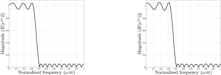
Figure 15.6:  Magnitude of frequency responses of linear-phase FIR filters design via discretization and LP, using a fine grid (left) and a sparse grid (right).

15.3    Mixed Integer Programming

Mixed integer linear programming, also named mixed integer programming (MIP), consists of LP problems like (15.1) or (15.3) in which some or all the variables have integer values. Although typically each integer variable can take only a finite number of values—particularly when the variable is binary and hence takes only the values 0 or 1—MIP problems are more difficult to solve, since they are nonconvex. Moreover, they are NP-hard, which basically means that, in the worst case, only exhaustive search over all the values of the integer variables can guarantee the optimality of the computed solution. Using heuristics based on the branch and bound technique presented in this section, optimal or nearly-optimal solutions can be found quite often.

15.3.1    Problem Statement and LP Relaxation

For the purpose of presentation and without losing generality from an algorithmic viewpoint, as it will be clear later, we assume that all variables are integer, i.e., the MIP problems have one of the standard forms

$\begin{array}{cc}\begin{array}{ll}\min \hfill & {\mathbf{c}}^T\mathbf{x}\hfill \\ \hfill \mathrm{s.t}.& \mathbf{Ax}=b\hfill \\ \hfill & \begin{array}{cc}\mathbf{x}\ge 0,& x\in {\mathbb{Z}}^n\end{array}\hfill \end{array}& \begin{array}{ll}\max \hfill & {\mathbf{e}}^T\mathbf{y}\hfill \\ \hfill \mathrm{s.t}.& \mathbf{Dy}\le \mathbf{f}\hfill \\ \hfill & y\in {\mathbb{Z}}^m\hfill \end{array}\end{array}$

(15.52)

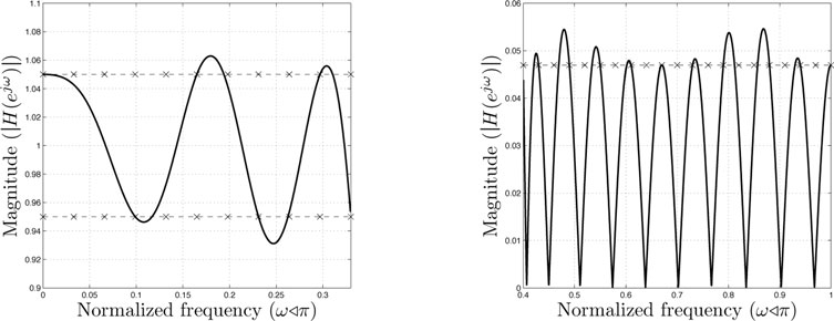
Figure 15.7:  Details of the frequency response obtained via discretization on a sparse grid: passband (left), stopband (right).

Such problems appear when the variables have naturally discrete numerical values or when they represent logical conditions. We start with a simple example; some sources of such problems are discussed in Section 15.3.3.

Example 15.3.1. Let us consider the following MIP problem:

$\begin{array}{llllll}\max \hfill & -\mathit{ϵ}{y}_1\hfill & +\hfill & y_2\hfill & \hfill & \hfill \\ \hfill \mathrm{s.t}.& -y_1\hfill & \hfill & \hfill & \le \hfill & -1\hfill \\ \hfill & \hfill y_1\hfill & +\hfill & y_2\hfill & \le \hfill & 8.2\hfill \\ \hfill & -y_1\hfill & -\hfill & 2y_2\hfill & \le \hfill & -3\hfill \\ \hfill & \hfill y_1\hfill & -\hfill & y_2\hfill & \le \hfill & 3\hfill \\ \hfill & -y_2\hfill & +\hfill & 5y_2\hfill & \le \hfill & 14\hfill \\ \hfill & \hfill y_1,\hfill & y_2\hfill & \in \hfill & \mathbb{Z}\hfill & \hfill \end{array}$

(15.53)

with ϵ a positive constant that is smaller than 0.2. Figure 15.8 illustrates the feasible domain, the gradient, and the level curves, for ϵ = 0.1. The gray area is the polygon defined by the inequality constraints of (15.53); the small circles represent the points with integer coordinates inside the polygon, hence they are the feasibility domain of the MIP problem; infeasible points with integer coordinates are marked with ×. We see from the level curves that the largest value of the criterion is obtained for y₁ = 1, y₂ = 3; so, this is the solution of (15.53).

For a problem of such small size, the solution can be found quickly by simple enumeration; for example, by realizing that 1 ≤ y₁ ≤ 5.5 and 0 ≤ y₂ ≤ 3, i.e., by covering the feasible set with a rectangle, we would have to check the 5 · 4 = 20 points with integer coordinates in this rectangle (some of which are infeasible). For problems with n variables, this exhaustive approach would need checking at least 2ⁿ points, in the favorable case where the variables are all binary. Obviously, this is computationally prohibitive in general.

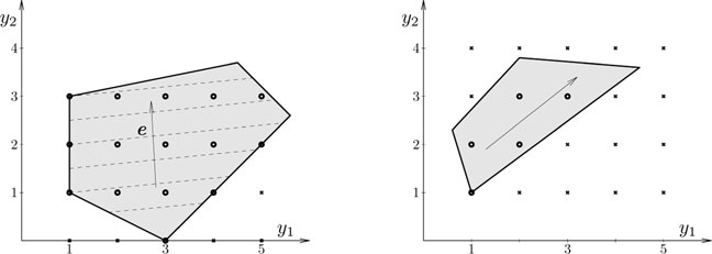
Figure 15.8:  Left: feasible points of the MIP problem from Example 15.3.1. Right: any rounding of the LP solution may produce an infeasible point.

Another naive approach would be to remove the integrality constraints, solve the relaxed resulting LP instead of the MIP, and then round the solution to integer values. In Example 15.3.1, the solution of the LP problem is y₁ = 4.5, y₂ = 3.7. Rounding to the nearest integer gives y = (4, 4) or y = (5, 4), which are not feasible points. Truncating gives y = (4, 3), which is feasible, but not optimal. In general, a y ∈ ℝⁿ is in a box with 2ⁿ vertices with integer coordinates (either $\lfloor y_i\rfloor$ or $\lceil y_i\rceil$, for each i = 1 : n), so the search of a feasible vertex is by itself difficult. Moreover, it is possible that none of the vertices is a feasible point, as suggested on the right of Figure 15.8; the solution of the LP problem is the rightmost vertex of the corresponding feasible polygon; none of the neighboring points with integer coordinates is a feasible point for the MIP problem. However, the idea of solving the LP problem is not at all worthless, as we will see next.

For some problems, it can be told by simple inspection of the problem that the LP solution is optimal for the MIP problem. Consider the assignment problem, in which ℓ agents have to execute simultaneously ℓ different tasks; so, an agent executes a single task and a task is executed by a single agent. The cost of executing task i by agent j is c_i,j. The purpose is to find the assignment with minimum cost. The problem can be modeled by introducing binary variables x_i,j, i, j = 1 : ℓ, with the meaning that x_i,j = 1 if task i is executed by agent j and x_i,j = 0 otherwise. The resulting MIP optimization problem is

$\begin{array}{ll}\min \hfill & {\displaystyle {\sum }_{i=1}^{\mathit{\ell }}{\displaystyle {\sum }_{j=1}^{\mathit{\ell }}{c}_{i,j}{x}_{i,j}}}\hfill \\ \hfill \mathrm{s.t}.& \begin{array}{cc}{\displaystyle {\sum }_{j=1}^{\mathit{\ell }}{x}_{i,j}=1,}& j=1:\mathit{\ell }\end{array}\hfill \\ \hfill & \begin{array}{cc}{\displaystyle {\sum }_{j=1}^{\mathit{\ell }}{x}_{i,j}=1,}& i=1:\mathit{\ell }\end{array}\hfill \\ \hfill & \begin{array}{cc}{x}_{i,j}\in \left\{0,1\right\},& i,j=1:\mathit{\ell }\end{array}\hfill \end{array}$

(15.54)

The first constraint ensures that agent j executes exactly one task; the second constraint ensures that task i is executed by a single agent. The problem (15.54) can be relaxed to LP by replacing the binary constraints with 0 ≤ x_i,j ≤ 1. Hence, instead of searching the solution among the vertices of a hypercube in ℝⁿ (n = ℓ²), whose coordinates are either 0 or 1, the search is performed on the whole hypercube. Since the solution of the LP problem is a vertex of its feasible domain and all vertices have binary coordinates, the solution is also in the feasible domain of the MIP problem.

In degenerate cases, a numerical solver may return non-binary results; for example, if for some i₁, i₂, j₁, j₂ it happens that $c_{i_1,j_1}=c_{i_1,j_2}$ and $c_{i_2,j_1}=c_{i_2,j_2}$, then there is no preference in assigning tasks i₁ and i₂ to agents j₁ and j₂. Real results could be obtained from an LP solver for the corresponding variables $x_{i_1,j_1}$, $x_{i_1,j_2}$, but any rounding to {0, 1} that satisfies the constraints of (15.54) gives an optimal solution to the MIP problem.

In general, the LP relaxation gives the optimal MIP solution only if all vertices of its feasible polytope have integer coordinates. This happens quite seldom. For instance, assume that, in the assignment problem, agent j needs some resources r_ij to execute task i; bounding the total resources by a constraint ${\displaystyle {\sum }_{i=1}^{\mathit{\ell }}{\displaystyle {\sum }_{i=1}^{\mathit{\ell }}{r}_{i,j}{x}_{i,j}\le \rho }}$ will destroy the nice properties of problem (15.54), since the new constraint will probably “cut” a part of the hypercube and introduce new vertices with non-integer coordinates to the feasible polytope of the LP problem.

Still, the LP relaxation is at the core of the branch and bound method and hence is extremely useful.

15.3.2    Branch and Bound

Branch and bound is a general algorithmic idea based on a divide and conquer strategy. It is the background algorithm for the most successful MIP solvers. In this section, we will describe its basics and point out refinement directions whose details can be found in the specialized literature. Also, we do not discuss other algorithmic approaches to MIP, such as the cutting plane technique.

In MIP, branch and bound consists of solving LP problems with more and more constraints that restrain the feasibility domain, with the ultimate aim of providing integer solutions. The LP problems are seen as the nodes of a tree, as suggested in Figure 15.9. Once a problem is solved, two complementary constraints are added to it, producing two subproblems; this is called branching. Whenever possible, the information available from the LP solutions is used for deciding that further branching on a node cannot give the optimum, and hence stopping the search in the node without exploring its subtree; this is called bounding in general, but in MIP the common expression is that the node was fathomed.

We will describe the algorithm for the maximization (inequality) problem on the right of (15.52) and illustrate it for the problem (15.53), with ϵ = 0.1. By removing the integrality constraints from these problems we obtain an LP problem, denoted (P), whose solution and optimal value are y* and z, respectively; for (15.53), these are y* = (4.5, 3.7) and z = 3.25. Since the MIP problem is more constrained, it results that its optimal value cannot be larger than z. The branch and bound algorithm updates an upper bound z_max and a lower bound z_min to the MIP value; after solving (P), we can set z_max = z. However, there is no information on the lower bound, so we can only say that z_min = −∞, i.e., the value for an infeasible MIP problem.

Figure 15.9:  Branch and bound tree.

Typically, the solution of (P) is not integer, and this is indeed the case in our example, so further exploration is needed. Branching is performed by selecting one variable, say y₁, and adding to (P) the constraints $y_1\le \lfloor y_1^{\star }\rfloor$ and $y_1\ge \lceil y_1^{\star }\rceil$ to obtain two subproblems, denoted (P₀) and (P₁), respectively. Formally, we will write $\left(P_0\right)=\left(P,y_1\le \lfloor y_1^{\star }\rfloor \right)$ and $\left(P_1\right)=\left(P,y_1\ge \lceil y_1^{\star }\rceil \right)$. This choice is guided not only by the purpose of getting subproblems with smaller feasible domains, but also by the hope to obtain an integer optimal value for y₁ when solving the subproblems, although as we have seen above this will not necessarily happen. In our example, the subproblems are (P₀) = (P,y₁ ≤ 4) and (P₁) = (P,y₁ ≥ 5); their feasible domains are shown on the left of Figure 15.10; since it is no longer possible to have 4 < y₁ < 5, a part of the initial feasible domain has been eliminated. Since no feasible points with integer coordinates have been eliminated, the solution of the initial MIP problem is the solution of the MIP version of one of (P₀) or (P₁).

We go on by solving the subproblems. The solution of (P₀) is $y_0^{\star }=\left(4,3.6\right)$, and the optimal value z₀ = 3.2. Although z₀ < z_max, we cannot yet lower the upper bound of the MIP value to z₀, because it is possible that (P₁) gives a value larger than z₀. The solution is still noninteger, so we continue the branching, this time using the variable y₂ (however, in general one can branch several times on the same variable). The corresponding subproblems are $\left(P_{00}\right)=\left(P_0,y_2\le \lfloor {\left(y_0^{\star }\right)}_2\rfloor \right)$ and $\left(P_{01}\right)=\left(P_0,y_2\ge \lceil {\left(y_0^{\star }\right)}_2\rceil \right)$. For our example, they are $\left(P_{00}\right)=\left(P,y_1\le 4,y_2\le 3\right)$ (see right of Figure 15.10) and (P₀₁) = (P, y₁ ≤ 4, y₂ ≥ 4).

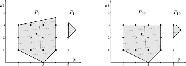
Figure 15.10:  Branch and bound subproblems. Left: after first branching, on y₁. Right: feasible problems after second branching, on y₂.

We have now three active (not solved) subproblems: (P₁), (P₀₀), (P₀₁). Any of them can be solved now, following diverse strategies of exploring the branch and bound tree. If (P₁) is solved first, the solution is $y_1^{\star }=\left(5,3.2\right)$ and the optimal value z₁ = 2.7. Branching continues with $\left(P_{10}\right)=\left(P_1,y_2\le \lfloor {\left(y_1^{\star }\right)}_2\rfloor \right)$ and $\left(P_{11}\right)=\left(P_1,y_2\ge \lceil {\left(y_1^{\star }\right)}_2\rceil \right)$. For our example, the subproblems are (P₁₀) = (P, y₁ ≥ 5, y₂ ≤ 3) and (P₁₁) = (P, y₁ ≥ 5, y₂ ≥ 4). We can set z_max = max(z₀, z₁) = 3.2, since none of the subproblems of (P₀) and (P₁) can have a value larger than that of their parents.

The LP problem (P₀₀) has the integer solution $y_{00}^{\star }=\left(1,3\right)$, with value z₀₀ = 2.9. Since we have found a feasible point for the initial MIP problem, we can set z_min = z₀₀. For the same reason, further branching on P₀₀ is not necessary. Although we actually have found the optimum, we cannot yet decide that this is indeed the case without examining the remaining active subproblems. The problem P₀₁ is infeasible, hence again there is no reason to branch. At this point we can update the upper bound as z_max = max(z₀₀, z₀₁, z₁) = 2.9. Since z_min = z_max, it results that $y_{00}^{\star }$ is the solution of the initial MIP problem. It is no longer necessary to explore (P₁₀) and (P₁₁).

If (P₀₀) and (P₀₁) are solved before (P₁), i.e., the search is organized depth-first, then, when solving (P₁), we notice that z₁ < z_min = z₀₀. Since the (noninteger) solution of (P₁) is worse than a currently available integer solution, nothing better can come from branching (P₁); so, the search on that subtree is stopped.

From the discussion above, we conclude that there are three situations when a node is considered fathomed:

•  the solution of the corresponding LP problem is integer (if the value of the LP problem is larger than z_min, then z_min is set to this value);

•  the LP problem is infeasible;

•  the value of the LP problem is smaller than the best value (stored in z_min) of an already found integer solution.

Based on the above discussion, a general form of the branch and bound algorithm for solving MIP problems is given in Table 15.3. The LP problem corresponding to a node of the branch and bound tree is solved in step 1. Fathomed nodes are discovered in steps 2 and 3. Branching is performed in step 4. In step 5, the value of z_max is updated using the following remark: if both LP subproblems of a node are solved, their values are less than or equal to the value of the LP problem corresponding to the node; the latter becomes an obsolete upper bound and can be ignored from now on. Finally, step 6 contains the conclusions; if the lower and upper bounds are equal, then the optimum has been found and the other active subproblems can remain unsolved; if there are no more active subproblems, then the only possibility is that z_min = −∞, i.e., no feasible integer point has been found for the MIP problem, which is hence infeasible.

Table 15.3:  Basic form of the branch and bound algorithm for solving MIP problems.

Input data: A, b, c of the MIP problem (15.52) in inequality form. Initialization. Create list $\mathcal{L}$ of active LP subproblems and initialize it with (P), the initial MIP problem without integrality constraints. Initialize lower and upper bounds to the optimal value: zmax = ∞, zmin = −∞. Create empty list ℳ of solved subproblems whose value may be zmax. Step 1. Choose a subproblem (S) from $\mathcal{L}$ and find its solution y* and value z. Remove (S) from $\mathcal{L}$. Append (S) to $\mathcal{M}$. Step 2. If z ≤ zmin, then either (S) is infeasible (z = −∞) or its value is too small for branching to produce good candidates to the optimum. Go to step 5. Step 3. If y* ∈ ℤm, then (since z > zmin), set zmin = z and y*MIP = y*. Go to step 5. Step 4. If y* ∉ ℤm, then choose a variable yi on which to branch. Create subproblems $\left(S_0\right)=\left(S,y_i\le \lfloor y_i^{\star }\rfloor \right)$, $\left(S_1\right)=\left(S,y_i\ge \lceil y_i^{\star }\rceil \right)$ and add them to $\mathcal{L}$. Step 5. Let (Sup) be the parent of (S). If both subproblems of (Sup) are in $\mathcal{M}$ (i.e., are both solved), remove (Sup) from $\mathcal{M}$. Update zmax as the maximum value of a problem from $\mathcal{M}$. Step 6. If zmin = zmax, then the MIP optimum has been found, stop. If the list $\mathcal{L}$ is empty, then the MIP problem is infeasible, stop. Otherwise, go back to step 1. Output: the MIP solution y*MIP and the corresponding optimal value zmin.

The fine details that make the difference between the branch and bound methods are in the choice of the next LP problem to be solved (step 1) and in the choice of the variable on which to branch (step 4). Both are guided by heuristics and can never guarantee a certain complexity of the algorithm. However, there are classes of problems that are favored by some algorithms. So, although MIP is a hard problem in general, branch and bound can give solutions in reasonable time if the number of variables m is relatively small. If m is larger than, say, 100, the complexity can easily explode, although current programs can solve even problems with thousands of variables. Anyway, the branch and bound algorithm can be stopped with a suboptimal solution, if z_min is deemed sufficiently close to z_max and hence can give useful information.

To give a taste of the different choices in step 1, let us first note that any order of exploration of the tree from Figure 15.9 is valid, as long as a node is examined before its subnodes. A depth-first search has the advantage of finding earlier terminal nodes with feasible integer solutions; they can give valuable information on the lower bound, hence z_min can grow rapidly. Another advantage is that the LP subproblems of a node are very similar with the problem in the node, since only one constraint is added to it; the simplex algorithm can be started with a good initial guess and it will have a very low complexity. A breadth-first search, that first explores all nodes at the same level in the tree, has the advantage of updating the upper bound z_max. Since these search strategies have complementary advantages, practical algorithms combine them, with the purpose of quickly narrowing the gap between z_min and z_max.

If the variables are binary, the branch and bound algorithm can be further refined, and its complexity is lower than that of a general MIP with the same number of variables and the same constraints. That is, the a priori information that the variables are binary can be used algorithmically.

Finally, note that if only some of the variables of the MIP problem have integer values, then the branch and bound algorithm works only on these variables. If optimality is detected with respect to integer variables, then the real variables also have optimal values.

15.3.3    Examples of Mixed Integer Problems

We describe here some problems whose modeling leads to MIP.

Logical conditions on LP constraints. The constraints of an optimization problem are implicitly connected by a logical AND. All of them must be satisfied by the solution. A natural question is how to model other logical operations. Consider first the case of an exclusive OR operation: an LP problem has some mandatory constraints Ax ≤ b and either one of the constraints

$\begin{array}{l}{\mathbf{A}}_1\mathbf{x}\le {\mathbf{b}}_1,\\ {\mathbf{A}}_2\mathbf{x}\le {\mathbf{b}}_2.\end{array}$

(15.55)

If these are the only alternatives, then one can impose them separately in two LP problems; the solution giving the best criterion is the desired one; however, if several pairs of alternatives like (15.55) are present, it is no longer efficient to solve an LP problem for each combination of constraints (one from each pair). A general way of dealing with (15.55) is to introduce two binary decision variables ξ₁, ξ₂ and to impose simultaneously the constraints

$\begin{array}{l}{\mathbf{A}}_1\mathbf{x}\le {\mathbf{b}}_1+{\xi }_1{\mathbf{u}}_1,\\ {\mathbf{A}}_2\mathbf{x}\le {\mathbf{b}}_2+{\xi }_2{\mathbf{u}}_2,\\ \begin{array}{cc}{\xi }_1+{\xi }_2=1,& {\xi }_1,{\xi }_2\in \left\{0,1\right\},\end{array}\end{array}$

(15.56)

where u₁, u₂ are vectors with positive elements, chosen big enough such that the constraints A₁x ≤ b₁ + u₁, A₂x ≤ b₂ + u₂ are satisfied for all desirable values of x; typically, all elements of u₁, u₂ are taken equal to a large constant M, and building (15.56) is called the “big-M” technique. The constraint ξ₁ + ξ₂ = 1 of the resulting MIP problem forces only one of the variables ξ₁ or x₂ to be zero, hence imposing only one of the constraints (15.55). In this case, since ξ₂ = 1 − ξ₁, one can use a single binary variable; for a generalization, see Exercise 15.10.

Other logical conditions make little sense. Imposing that at most one of the conditions (15.55) is satisfied can be modeled by ξ₁ + ξ₂ ≥ 1, but the optimal solution of the MIP problem will likely give ξ₁ = ξ₂ = 1, i.e., the solution of the LP problem without any of the constraints (15.55). Imposing that at least one of the conditions (15.55) is satisfied can be modeled by ξ₁ + ξ₂ ≤ 1, but the solution should be the same as that obtained with (15.56), since the optimization criterion should be improved by giving up one of the constraints. Note also that, in practice, it is recommended to take M as small as possible, since very large values, although theoretically desirable, can affect the numerical accuracy of the solution.

Sparse solutions to LP feasibility problems. Assume that we seek a vector x ∈ ℝⁿ satisfying some linear constraints Ax ≤ b (the exact form of these constraints is not important), such that its number of non-zero elements (namely ‖x‖₀) is minimum. For example, we want to design an FIR filter like in Example 15.2.5, satisfying the constraints of (15.51), but, instead of optimizing the stopband error bound γ_s, we keep it fixed to a preset value and minimize the number of non-zero elements. Such an optimization makes sense for hardware devices where the filter implementation cost depends on the number of coefficients, while the performance requirements are known. There are many heuristics for finding suboptimal solutions, like minimizing |x|₁ instead of ‖x‖₀ (see a similar idea in Example 15.2.2) or using greedy approaches that find the non-zero elements one by one [9]. Using the big-M technique, the minimization of ‖x‖₀, subject to Ax ≤ b, can be transformed into the equivalent MIP problem with binary variables

$\begin{array}{ll}\min \hfill & {\displaystyle {\sum }_{i=1}^n{\xi }_i}\hfill \\ \hfill \mathrm{s.t}.& \mathbf{Ax}\le \mathbf{b}\hfill \\ \hfill & \begin{array}{cc}-{\xi }_{i}M\le x_i\le {\xi }_{i}M,& i=1:n\end{array}\hfill \\ \hfill & \begin{array}{cc}{\xi }_i\in \left\{0,1\right\},& i=1:n\end{array}\hfill \end{array}$

(15.57)

Taking M big enough, if the binary variable ξ_i is zero, then x_i is also zero. If ξ_i = 1, then x_i, is practically unrestricted. Hence, the optimization criterion is the number of non-zero elements of x.

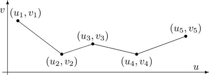
Figure 15.11:  Piecewise linear function.

Piecewise linear constraint. Consider two scalar variables, u and v, linked by a piecewise linear relation like in Figure 15.11, with given points (u_i, v_i), i = 1 : p. To model such a nonconvex constraint in MIP style, we start by noticing that a segment is made by all convex combinations of its end points. If u and v belong to the segment i connecting (u_i, v_i) and (u_i+1, v_i+1), then they satisfy the relations

$\begin{array}{l}u=\xi u_i+\zeta u_{i+1},\\ v=\xi v_i+\zeta v_{i+1},\end{array}$

(15.58)

with ξ + ζ =1 and ξ, ζ ≥ 0. Since the variable point (u, v) can be on an arbitrary segment, we have to introduce real variables ξ_i, ζ_i for each segment i = 1 : p − 1 and model the piecewise linear relation through

$\begin{array}{l}u={\displaystyle {\sum }_{i=1}^{p-1}\left[{\xi }_i{u}_i+{\zeta }_i{u}_{i+1}\right]},\\ v={\displaystyle {\sum }_{i=1}^{p-1}\left[{\xi }_i{v}_i+{\zeta }_i{v}_{i+1}\right]},\end{array}$

(15.59)

where all pairs ξ_i, ζ_i are zero, except one, since (u, v) may belong to only one segment. This constraint can be modeled with binary variables η_i, i = 1 : p − 1, by imposing

$\begin{array}{l}{\xi }_i+{\zeta }_i={\eta }_i,\\ \begin{array}{ccc}{\xi }_i\ge 0,& {\zeta }_i\ge 0,& i=1:p-1\end{array}\\ {\displaystyle {\sum }_{i=1}^{p-1}{\eta }_i=1,}\\ \begin{array}{cc}{\eta }_i\in \left\{0,1\right\},& i=1:p-1.\end{array}\end{array}$

(15.60)

So, only one of the binary variables η_i can be one, the others being zero; then, only one pair of variables ξ_i, ζ_i is non-zero and obeys to ξ_i+ζ_i = 1, the others being zero. The constraints (15.59) and (15.60) are linear and depend on the real variables u, v and ξ_i, ζ_i, i = 1 : p − 1, and the binary variables η_i, i = 1 : p − 1, so they can be indeed inserted in a MIP problem. This model is not the most economic: the number of real variables can be reduced to almost a half, as described in [10] and suggested in Exercise 15.11; however, the complexity of solving the MIP problem is dictated mostly by the number of integer variables.

Design of FIR filters with signed power-of-two coefficients. We consider here the FIR filter design problem in Example 15.2.5 from a new angle, that of minimizing its hardware implementation complexity, which is very useful when designing specialized circuits. An important part of the implementation cost is dictated by the physical realization of the coefficients of the filter (15.49), which are implemented with finite precision. We have seen above that one can minimize the number of non-zero coefficients, but here we consider a more detailed description of the coefficients. In fixed point arithmetic, a coefficient h_k can be represented as

$h_k={\displaystyle \sum _{i=-\alpha }^{\beta }{h}_{ik}{2}^i},$

(15.61)

where h_ik ∈ {−1, 0, 1} are signed digits in a binary representation with p = α+β +1 digits, that covers β + 1 digits in the integer part and α digits in the fractional part. The value of β dictates the maximum magnitude and can have small values like 1 or 2 and the value of α sets the precision of the implementations and can be 8–10 or even larger. The relation (15.61) is called signed power-of-two (SPT) representation. Note that, unlike the canonical representation that admits only the digits 0 and 1 and has a separate representation of the sign, the SPT representation is not unique; for example, the decimal number 0.375 can be represented as 2⁻² + 2⁻³ or 2⁻¹ − 2⁻³.

Using the notations from Example 15.2.5, the frequency response of the filter is essentially given by

$\mathbf{a}{\left(\omega \right)}^T\mathbf{h}={\displaystyle \sum _{k=0}^n{h}_k{a}_k\left(\omega \right)}={\displaystyle \sum _{k=0}^n{\displaystyle \sum _{i=-\alpha }^{\beta }{h}_{ik}{2}^i{a}_k\left(\omega \right)=\mathbf{b}{\left(\omega \right)}^T\mathbf{y}}}$

where a_k(ω) = 2 cos(n − k)ω, k = 0 : n − 1, α_n(ω) = 1, and

$\begin{array}{cccccc}{\mathbf{y}}^T=[h_{-\alpha ,0}& \dots & h_{\beta ,0}& h_{-\alpha ,1}& \dots & h_{\beta ,n}],\\ \mathbf{b}{\left(\omega \right)}^T=\left[2^{-\alpha }{a}_0\left(\omega \right)\right]& \dots & 2^{\beta }{a}_0\left(\omega \right)& 2^{-\alpha }{a}_1\left(\omega \right)& \dots & 2^{\beta }{a}_n\left(\omega \right)].\end{array}$

So, the frequency response depends linearly on the unknown vector y ∈ ℝ^p(n+1). Hence, by imposing tolerances γ_ρ and γ_s and minimizing the number of nonzero bits of the SPT representation of the filter coefficients, the discretized LP design problem (15.51) can be transformed into the MIP problem

$\begin{array}{ll}\min \hfill & {\Vert \mathbf{y}\Vert }_1\hfill \\ \hfill \mathrm{s.t}.& \begin{array}{cc}1-{\gamma }_p\le \mathbf{b}{\left({\omega }_{\mathit{\ell }}\right)}^T\mathbf{y}\le 1+{\gamma }_p,& \mathit{\ell }=1:L_p,\end{array}\hfill \\ \hfill & \begin{array}{cc}-{\gamma }_s\le \mathbf{b}{\left({\omega }_{\mathit{\ell }}\right)}^T\mathbf{y}\le {\gamma }_s,& \mathit{\ell }=L_p+1:L_p+L_s\end{array}\hfill \\ \hfill & \mathbf{y}\in {\left\{-1,0,1\right\}}^p{}^{\left(n+1\right)}\hfill \end{array}$

(15.62)

Other linear constraints can be added to this problem. For example, if the number of non-zero bits per coefficient has to be bounded to p̃, the constraint is

$\begin{array}{cc}{\displaystyle \sum _{i=-\alpha }^{\beta }\left|h_{ik}\right|}\le \tilde{p},& k=0:n.\end{array}$

The redundancy of the SPT representation is eliminated if two non-zero bits are never consecutive, which can be written as

$\begin{array}{ccc}\left|h_{ik}\right|+\left|h_{i+1,k}\right|\le 1,& i=-\alpha :\beta -1,& k=0:n.\end{array}$

Although this increases the number of constraints, it actually reduces the execution time in many cases. The above condition also slightly reduces the range of the coefficients: the larger value is no longer 2^β + 2^β−1 + … + 2^−α = 2^β+1 − 2^−α, but 2^β + 2^β−2 + 2^β−4 + …; however, inside the new range, all values multiple of 2^−α are attainable.

Alternatively to the SPT representation, one could replace (15.61) with the standard fixed point representation

$\begin{array}{cc}{h}_k=x_k\cdot 2^{-\alpha },& x_k\in \mathbb{Z},\left|x_k\right|\le 2^p-1.\end{array}$

(15.63)

Although the result of the corresponding MIP optimization problem can be easily converted to SPT representation, some constraints cannot be posed on the representation (15.63), for example those regarding the number of non-zero bits. However, (15.63) is useful when the coefficients are optimized for a software implementation of the filter in fixed point arithmetic, where the only constraints regard the range and precision of the coefficients, not the particular values of their bits.

15.4    Historical Notes and Further Reading

Although there are earlier descriptions, the first treatment of linear programming as a distinct optimization problem belonged to L.V. Kantorovich in 1939, in relation with production planning. In 1947, G.B. Dantzig invented the simplex method, the first efficient tool for solving LP problems on a computer. The next 30 years brought different improvements to the simplex method, without changing its basic principles, together with the understanding of its exponential complexity. In 1979, L.G. Khachiyan [11] presented the ellipsoid method, which was the first polynomial time algorithm, with a O(n⁴) complexity; however, in practice the algorithm was always worse than the simplex, as its average complexity was near the worst case one. The first efficient interior-point algorithm, with a theoretical complexity of O(n^3.5), but usually much better, was given by N. Karmarkar [12] in 1984, giving a huge impulse on the research of interior-point algorithms with general use in several classes of convex optimization. Currently, the simplex and interior-point methods are considered of practically equal importance, each being possibly better for LP problems with different characteristics and provenance.

More historical information, with emphasis on interior-point methods can be found in [13], [2], and [14]. An early simple presentation of the interior-point method and comparisons with the simplex method can be found in [15]. The reader interested in more detailed presentations of linear programming can consult textbooks like [10] and [16]. LP belongs to the more general category of convex optimization, treated extensively in [17].

Mixed integer programming belongs essentially to combinatorial optimization, where branch and bound is the preferred algorithmic tool. As such, solving MIP problems via branch and bound was not especially innovative in principle; however, there are many methods that cleverly take advantage of the particular connection with LP. For a broader view on the field, see for example [18].

There are many software packages for solving LP and MIP problems. The reader is encouraged to try noncommercial software like LP_SOLVE, GPLK or MINTO. Semidefinite programming solvers can be easily used for LP problems; packages like SeDuMi, SDPT3, CVX, Yalmip are all free and the latter has also a MIP module.

15.5    Exercises

Exercise 15.1. Consider the problem of minimizing Re (c^Tx), with the constraint Ax = b, where the variable x and the data A, b, c are complex. Assuming that the real and imaginary parts of x are non-negative, transform it into the standard form (15.1).

Exercise 15.2. Is there a value of c such that all feasible points of problem (15.2) are also solutions? In general, show that if c ∈ $\mathcal{I}$m (A^T), then all feasible points are optimal, i.e., have the same value c^Tx. Hint: express the solutions of the linear system Ax = b as x = x₀ + u, with x₀ a particular solution and u ∈ $\mathcal{K}$er (A).

Exercise 15.3. Consider the LP primal problem (15.1) with A = [−1 0], b = 1, c = [0 − 1]^T. Show that both the primal and its dual (15.9) are infeasible.

Exercise 15.4. Show that the dual of the optimization problem (15.3) is

$\begin{array}{ll}\min \hfill & {\mathbf{f}}^T\mathbf{x}\hfill \\ \hfill \mathrm{s.t}.& {\mathbf{D}}^T\mathbf{x}=\mathbf{e}\hfill \\ \hfill & \mathbf{x}\ge 0\hfill \end{array}$

which means that the dual of the dual of the primal LP problem (15.1) is the primal itself.

Exercise 15.5. An LP problem in the form

$\begin{array}{ll}\max \hfill & {\mathbf{c}}^T\mathbf{x}\hfill \\ \hfill \mathrm{s.t}.& \mathbf{Ax}\le \mathbf{b}\hfill \\ \hfill & \mathbf{x}\ge 0\hfill \end{array}$

is also called standard. Show that its dual is

$\begin{array}{ll}\min \hfill & {\mathbf{b}}^T\mathbf{y}\hfill \\ \hfill \mathrm{s.t}.& {\mathbf{A}}^T\mathbf{y}\ge \mathbf{c}\hfill \\ \hfill & \mathbf{y}\ge 0\hfill \end{array}$

If b > 0, after introducing slack variables to transform the problem into the form (15.1), find a basic feasible point.

Exercise 15.6. Strong duality of LP is basically equivalent to Farkas’ lemma (see page 526 for its statement) used in the proof of Theorem 15.1.6. Prove Farkas’ lemma by applying Theorem 15.1.6 to the LP program:

(i) Primal (feasibility problem): min 0, subject to Φu = f, u ≥ 0.

Hint: show that its dual is

(ii) max f^Tv, subject to Φ^Tv ≤ 0 (note that the inequality is opposite to that on page 526).

Use the facts that: (a) if the primal is feasible, then the value of (ii) is zero; (b) if there is a feasible v such that f^Tv > 0, then the dual is unbounded, hence the primal is infeasible.

Exercise 15.7. Express as LP in standard equality form the problem of minimizing ‖x‖₁ or ‖x‖_∞ subject to the equality constraint Ax = b. If A ∈ ℝ^m×n, then the matrix of the standard LP problem (15.1) should have size m × 2n for the 1-norm minimization and (m + n) × (2n + 1) for the ∞-norm minimization. (Hint: for the 1-norm, use the substitution x = x₊ − x₋ and show that, at optimality, x₊ and x₋ cannot have non-zero elements in the same position.)

Exercise 15.8. Assume that the positions (x_i, y_i) of N points in ℝ² are given. Express as LP the problem of finding a polynomial $f\left(x\right)={\displaystyle {\sum }_{k=0}^n{a}_k{x}^k}$ such that the maximum error |y_i − f(x_i)|, i = 1: N, is minimum.

Exercise 15.9. Consider an LP problem which, together with some mandatory constraints, is also constrained to exactly one of the equalities A₁x = b₁, A₂x = b₂. Model this problem as MIP. (Hint: transform each equality into inequalities, then apply the big-M technique.)

Exercise 15.10. Consider an LP problem in which exactly L of the N conditions A_ix ≤ b_i, i = 1 : N, should be satisfied, with A_i, b_i given matrices and vectors of appropriate sizes. How can it be modeled as a MIP problem?

Exercise 15.11. Alternatively to (15.59), the piecewise linear function from Figure 15.11 can be modeled via only p variables θ_i through the relations

$\begin{array}{l}u={\displaystyle {\sum }_{i=1}^p{\theta }_i{u}_i},\\ v={\displaystyle {\sum }_{i=1}^p{\theta }_i{v}_i},\end{array}$

where θ_i ≥ 0, ${\displaystyle {\sum }_{i=1}^p{\theta }_i=1}$; each variable θ_i is associated with a point (u_i, v_i); since the variables (u, v) belong to a single segment i, then only the variables θ_i and θ_i+1 must be non-zero (their sum being equal to one) and the others must be zero.

Prove that, together with the above, the conditions

$\begin{array}{l}{\theta }_1\le {\eta }_1\\ \begin{array}{cc}{\theta }_i\le {\eta }_{i-1}+{\eta }_i,& i=2:p-1\end{array}\\ {\theta }_p\le {\eta }_{p-1}\\ {\displaystyle {\sum }_{i=1}^{p-1}{\eta }_i=1}\\ \begin{array}{cc}{\eta }_i\in \left\{0,1\right\},& i=1:p-1\end{array}\end{array}$

describe correctly the piecewise linear dependence. (Hint: note that variable η_i corresponds to segment i and η_i + η_i = 1 only for two consecutive values i.)

Exercise 15.12. We want to place N objects on the floor of a rectangular room. Each object has a rectangular basis, so we can model the problem in 2D; the length ℓ_i and width w_i of object i are given; the height is not relevant, since the objects cannot be superposed. The position of object i is given by the coordinates (x_i, y_i) of one of its corners, the same for all objects.

What is the condition that objects i and j occupy distinct positions in space (their basis rectangles do not superpose)?

How can this condition be modeled in the constraints of an optimization problem (the criterion is not relevant now)?

References

[1]   V. Klee and G. Minty, “How good is the simplex method,” in Inequalities III, O. Shisha, Ed. Academic Press, 1972, pp. 159–175.

[2]   M. Todd, “The many facets of linear programming,” Math. Program. Ser. B, vol. 91, no. 3, pp. 417–436, Feb. 2002.

[3]   R. Bartels and G. Golub, “The simplex method of linear progamming using LU decomposition,” Comm. ACM, vol. 12, no. 5, pp. 266–268, May 1969.

[4]   J. Picard and A. Weiss, “Bounds on the Number of Identifiable Outliers in Source Localization by Linear Programming,” IEEE Trans. Signal Proc., vol. 58, no. 5, pp. 2884–2895, May 2010.

[5]   W. Zhou, L. Zhang, and L. Jiao, “Linear programming support vector machines,” Pattern Recognition, vol. 35, pp. 2927–2936, 2002.

[6]   B. Dumitrescu, Positive Trigonometric Polynomials and Signal Processing Applications. Springer, Dordrecht, The Netherlands, 2007.

[7]   R. Reemtsen and J.-J. Rückman, Eds., Semi-Infinite Programming. Kluwer Academic Publishers, Dordrecht, The Netherlands, 1998.

[8]   M. Goberna and M. Lopez, “Semi-infinite programming theory: an updated survey,” Eur. J. Operational Research, vol. 143, pp. 390–405, 2002.

[9]   T. Baran, D. Wei, and A. Oppenheim, “Linear programming algorithms for sparse filter design,” IEEE Trans. Signal Proc., vol. 58, no. 3, pp. 1605–1617, March 2010.

[10]   D. Bertsimas and J. Tsitsiklis, Introduction to Linear Optimization. Athena Scientific, Nashua, NH, USA, 1997.

[11]   L. Khachiyan, “A polynomial algorithm in linear programming,” Soviet Math. Dokl., vol. 20, pp. 191–194, 1979.

[12]   N. Karmarkar, “A new polynomial-time algorithm for linear programming,” Combinatorica, vol. 4, no. 4, pp. 373–395, 1984.

[13]   R. Freund and S. Mizuno, “Interior point methods: current status and future directions,” in High Performance Optimization, H. F. et al., Ed. Kluwer Academics, pp. 441–466, 2000.

[14]   M. Wright, “The interior-point revolution in optimization: history, recent developments, and lasting consequences,” Bull. Amer. Math. Soc., vol. 42, no. 1, pp. 39–56, 2005.

[15]   G. Astfalk, I. Lustig, R. Marsten, and D. Shanno, “The interior-point method for linear programming,” IEEE Software, vol. 9, no. 4, pp. 61–68, July 1992.

[16]   R. Vanderbei, Linear Programming: Foundations and Extensions, 2nd ed. Springer, New York, NY, USA, 2001.

[17]   S. Boyd and L. Vandenberghe, Convex Optimization. Cambridge University Press, Cambridge, UK, 2004.

[18]   L. Wolsey and G. Nemhauser, Integer and Combinatorial Optimization. Wiley-Interscience, New York, NY, USA, 1999.