Chapter 11  Fundamentals of Detection Theory

Venugopal V. Veeravalli^‡

^‡ University of Illinois at Urbana-Champaign, USA

11.1    Introduction

Detection problems arise in a number of engineering applications such as radar, communications, surveillance, and image analysis. In the basic setting of the problem, the goal is to detect the presence or absence of a signal in noise. This chapter will provide the mathematical and statistical foundations for solving such problems.

11.1.1    Statistical Decision Theory Framework

Detection problems fall under the umbrella of statistical decision theory [1], where the goal is to make a right (optimal) choice from a set of alternatives in a noisy environment. There are five basic ingredients in a typical decision theory problem.

•  $\mathcal{S}$: The set of states (of nature). For detection problems, the number of states is finite, i.e., ∣$\mathcal{S}$∣ = M < ∞. For binary detection problems, which are prevalent in applications, $\mathcal{S}$ = {0, 1}. We denote a typical state for detection problems by the variable j, i.e., j ∈ $\mathcal{S}$.

•  $\mathcal{D}$: The set of decisions or actions. This set is the set of decisions about the state. Elements in $\mathcal{D}$ would typically correspond to elements in $\mathcal{S}$. In some applications such as communications with erasure, the set $\mathcal{D}$ could have larger cardinality than the set $\mathcal{S}$. We denote a typical decision by the variable i, i.e., i ∈ $\mathcal{D}$.

•  C(i, j) or C_i,j: The cost function between decisions and states, C : $\mathcal{D}$ × $\mathcal{S}$ → ℝ⁺. In order to be able to talk about optimizing the decision, we need to quantify the cost incurred from each decision. The cost function C serves this purpose. An example of cost function, which is relevant in many applications, is the uniform cost function for which

$C_{i,j}=\{\begin{array}{cc}0& \mathrm{if}i=j\\ 1& \mathrm{if}i\ne j\end{array}.$

(11.1)

•  $\mathcal{Y}$: The set of observations. The decision about the state is not made blindly but based on some random observation¹ Y taking values in $\mathcal{Y}$.

•  Δ: The set of decision rules or tests. Since the decisions are based on the observations, we need to have mappings from the observation set to the decision set. These are the decision rules, i.e., δ ∈ Δ, δ : $\mathcal{Y}$ ↦ $\mathcal{D}$.

Detection problems are also referred to as hypothesis testing problems, with the understanding that each element of $\mathcal{S}$ corresponds to a hypothesis about the nature of the observations. The hypothesis corresponding to state j is denoted by H_j.

11.1.2    Probabilistic Structure for Observation Space

We associate with $\mathcal{Y}$, a sigma algebra $\mathcal{G}$ of subsets of $\mathcal{Y}$ to which we assign probabilities. The pair ($\mathcal{Y}$, $\mathcal{G}$) is the observation space. In the applications of interest in this chapter, we will almost exclusively have $\mathcal{Y}$ = $\mathbb{R}$ⁿ, or $\mathcal{Y}$ = {γ₁, γ₂, …}, a countable set. In the case that $\mathcal{Y}$ = ℝⁿ, we take $\mathcal{G}$ to be the smallest sigma-algebra containing all the n-dimensional rectangles in ℝⁿ, i.e., the Borel sigma-algebra $\mathcal{B}$ⁿ. In the case when $\mathcal{Y}$ = {γ₁, γ₂, …}, we take $\mathcal{G}$ to be the power set of $\mathcal{Y}$, i.e., 2^{$\mathcal{Y}$}.

For $\mathcal{Y}$ = Rⁿ, we assume that probabilities can be assigned using an n-dimensional PDF. For $\mathcal{Y}$ = {γ₁, γ₂, …}, probabilities can be assigned using a PMF. We will use the term density for both PDFs and PMFs. We denote this density function by p, and use a common notation for the probability measure as in [2]:

For A ∈ $\mathcal{G}$,

$P\left(A\right)={\displaystyle {\int }_{y\in A}p\left(y\right)\mu \left(dy\right)}=\{\begin{array}{cc}{\displaystyle {\int }_{y\in A}p\left(y\right)dy}& \mathrm{for}\mathcal{Y}={ℝ}^n\\ {\displaystyle {\sum }_{{\gamma }_i\in A}p\left({\gamma }_i\right)}& \mathrm{for}\mathcal{Y}=\left\{{\gamma }_1,{\gamma }_2,\dots \right\}\end{array}$

(11.2)

Let g be a function on $\mathcal{Y}$. Then the expected value of the random variable g(Y) is given by

$\mathrm{E}\left[g\left(Y\right)\right]={\displaystyle {\int }_{\mathcal{Y}}p\left(y\right)g\left(y\right)\mu \left(dy\right)}=\{\begin{array}{cc}{\displaystyle {\int }_{\mathcal{Y}}p\left(y\right)g\left(y\right)dy}& \mathrm{for}\mathcal{Y}={ℝ}^n\\ {\displaystyle {\sum }_{\mathcal{Y}}p\left({\gamma }_i\right)g\left({\gamma }_i\right)}& \mathrm{for}\mathcal{Y}=\left\{{\gamma }_1,{\gamma }_2,\dots \right\}\end{array}$

(11.3)

11.1.3    Conditional Density and Conditional Risk

In order to make a decision about the state j based on the observation Y, we need to know how Y depends on j statistically. Typically, we assume that the conditional density (PDF/PMF) of Y conditioned on the state being j (which we denote by p_j(y)) is available for each j ∈ $\mathcal{S}$. In case the state is modeled as random variable J (see below), p_j(y) is the usual conditional density p_Y∣J(y∣j), but otherwise we can think of the set {p_j(y), j ∈ $\mathcal{S}$} as simply an indexed set of densities, with p_j being the density for Y that corresponds to the state being j.

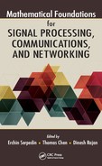
Table 11.1:  Decision rules and conditional risks for Example 11.1.1.

The cost associated with a decision rule δ ∈ Δ is a random quantity (because Y is random) given by C(δ(Y), j). Therefore, to order decision rules according to their “merit” we use the quantity

$R_j\left(\delta \right)=E_j\left[C\left(\delta \left(Y\right),j\right)\right]={\displaystyle \int C\left(\delta \left(y\right),j\right)p_j\left(y\right)\mu \left(dy\right)}.$

which we call the conditional risk associated with δ when the state is j.

The conditional risk function can be used to obtain a (partial) ordering of the decision rules in Δ, in the following sense.

Definition 11.1.1. A decision rule δ is better than decision rule δ′ if

$R_j\left(\delta \right)\le R_j\left({\delta }^{\prime }\right),\forall j\in \mathcal{S}$

and

$R_j\left(\delta \right)<R_j\left({\delta }^{\prime }\right),\mathrm{for}\mathrm{at}\mathrm{least}\mathrm{one}j\in \mathcal{S}$

Sometimes it may be possible to find a decision rule δ* ∈ Δ which is better than any other δ ∈ Δ. In this case, the statistical decision problem is solved. Unfortunately, this usually happens only for trivial cases as in the following example.

Example 11.1.1. Suppose $\mathcal{S}$ = $\mathcal{D}$ = {0, 1} with the uniform cost function as in (11.1). Furthermore suppose the observation Y takes values in the set $\mathcal{Y}$ = {a, b, c} and the conditional p.m.f.’s of Y are:

$p_0\left(a\right)=1,p_0\left(b\right)=p_0\left(c\right)=0,p_1\left(a\right)=0,p_1\left(b\right)=p_1\left(c\right)=\mathrm{0.5.}$

Then it is easy to see that we have the conditional risks for the eight possible decision rules depicted in Table 11.1. Clearly, δ₄ is the best rule according to Definition 11.1.1, but this happens only because the conditional PMFs p₀ and p₁ have disjoint supports (see Exercise 2).

□

Since conditional risks cannot be used directly in finding optimal solutions to statistical decision making problems except in trivial cases, there are two general approaches for finding optimal decision rules: Bayesian and minimax.

11.1.4    Bayesian Approach

Here we assume that we are given an a priori probability distribution on the set of states $\mathcal{S}$. The state is then denoted by a random variable J with PMF {π_j , j ∈ $\mathcal{S}$} (since, for detection problems, the state space is finite). Now we introduce the average risk or Bayes risk associated with a decision rule δ, which is given by

$r\left(\delta \right)=E\left[R_J\left(\delta \right)\right]={\displaystyle \sum _{j\in \mathcal{S}}{\pi }_j{R}_j}\left(\delta \right)$

(11.4)

We can then obtain an ordering on the δ’s by using this Bayes risk. In particular, we choose the decision rule δ_B that has minimum Bayes risk, i.e.,

${\delta }_{\text{B}} =\arg \underset{\delta \in \Delta }{\min }r(\delta ).$

The decision rule δ_B is called Bayes rule.

11.1.5    Minimax Approach

What if we are not given a prior distribution on the set $\mathcal{S}$? We could postulate a distribution on $\mathcal{S}$ (for example, a uniform distribution) and use the Bayesian approach. On the other hand, one may want to guarantee a certain level of performance for all choices of state. In this case, we use a minimax approach. The goal of the minimax approach is to find the decision rule δ_m that has the best worst case cost:

${\delta }_{\mathrm{m}}=\arg \underset{\delta \in \text{Δ}}{\min }\underset{j\in \mathcal{S}}{\max }{R}_j\left(\delta \right).$

The decision rule δ_m is called the minimax rule.

In addition to Bayes and minimax approaches there are other criteria and techniques that are specific to special classes of decision-making problems. For example, in binary hypothesis testing, a third approach called the Neyman-Pearson approach (see Section 11.4) is often used in practice.

11.1.6    Randomized Decision Rules

Even though this might seem counter-intuitive at first, it is sometimes possible to get a better decision rule by randomly choosing between a set of deterministic decision rules.

Definition 11.1.2. A randomized decision rule δ̃ is described by

$\tilde{\delta }\left(y\right)={\delta }_{\mathcal{l}}\left(y\right)\mathrm{with}\mathrm{probability}{\beta }_{\mathcal{l}},\mathcal{l}=1,\dots ,L$

for some L and some {β_ℓ}, with β_ℓ > 0 and ∑_ℓ ß_ℓ = 1.

Table 11.2:  Decision rules, and Bayes and minimax risks for Example 11.1.2.

The set Δ̃ of randomized decision rules obviously contains the set Δ, and thus optimizing over Δ̃ will necessarily result in at least as good a decision rule as that obtained by optimizing over Δ.

Theorem 11.1.1. Randomization does not improve Bayes rules:

$\underset{\delta \in \text{Δ}}{\min }r\left(\delta \right)=\underset{\tilde{\delta }\in \widetilde{\text{Δ}}}{\min }r\left(\tilde{\delta }\right).$

Proof: Since Δ ⊂ Δ̃, it is clear that the right-hand side (RHS) is less than or equal to the left-hand side (LHS). To prove the reverse inequality, suppose δ̃ chooses δ_ℓ with probability β_ℓ, ℓ = 1, …, L. Then

$r\left(\tilde{\delta }\right)={\displaystyle \sum _{\mathcal{l}=1}^L{\beta }_{\mathcal{l}}r\left({\delta }_{\mathcal{l}}\right)}\ge {\displaystyle \sum _{\mathcal{l}=1}^L{\beta }_{\mathcal{l}}}\underset{\delta \in \text{Δ}}{\min }r\left(\delta \right)=\underset{\delta \in \text{Δ}}{\min }r\left(\delta \right).$

Taking the minimum over δ̃ ∈ Δ̃ on the LHS gives us the desired inequality.

■

However, as we see in the following example, randomization could result in a better minimax rule. We will also see later in Section 11.4 that randomization can yield better Neyman-Pearson rules for binary detection problems.

Example 11.1.2. Consider the same setup as in Example 11.1.1 with the following conditional PMF’s.

$p_0\left(a\right)=p_0\left(b\right)=0.5,p_0\left(c\right)=0,p_1\left(a\right)=0,p_1\left(b\right)=p_1\left(c\right)=\mathrm{0.5.}$

We can compute the conditional risks for the eight possible decision rules as shown in Table 11.2. Clearly there is no “best” rule based on conditional risks alone in this case. Now consider finding a Bayes rule for priors π₀ = π₁ = 0.5. It is clear from the table that δ₂ and δ₄ are both Bayes rules. Also, δ₂, δ₃, δ₄ and δ₆ are all minimax rules with minimax risk equal to 0.5. Finally, randomizing between δ₂ and δ₄ with equal probability results in a rule with minimax risk equal to 0.25. Thus, we see that randomization can improve minimax rules.

□

11.1.7    General Method for Finding Bayes Rules

In the Bayesian framework, we can define the a posteriori probability π(j∣y) of the state j, given observation y. By Bayes probability law:

$\pi \left(j|y\right)=\frac{p_j\left(y\right){\pi }_j}{p\left(y\right)}.$

(11.5)

We can write the Bayes risk of (11.4) in terms of π(j∣y) as:

$r\left(\delta \right)=\text{E}\left[\mathrm{E}\left[C\left(\delta \left(Y\right),J\right)|Y\right]\right]={\displaystyle {\int }_{y\in \mathcal{Y}}\left[{\displaystyle \sum _{j\in \mathcal{S}}\pi \left(j|y\right)C\left(\delta \left(y\right),j\right)}\right]}p\left(y\right)\mu \left(dy\right).$

(11.6)

Define the a posteriori cost of decision i ∈ $\mathcal{D}$, given observation y, by

$C\left(i|y\right)\triangleq {\displaystyle \sum _{j\in \mathcal{S}}\pi \left(j|y\right)}C\left(i,j\right).$

(11.7)

Then it is easy to see that minimizing r(δ) in (11.6) is equivalent to minimizing C(δ(y)∣y) for each y. Thus

${\delta }_{\mathrm{B}}\left(y\right)=\arg \underset{i\in \mathcal{D}}{\min }C\left(i|y\right).$

(11.8)

11.2    Bayesian Binary Detection

We now study the special case of binary detection (hypothesis testing) in more detail. Here $\mathcal{S}$ = $\mathcal{D}$ = {0, 1}, and hence any deterministic decision rule δ partitions the observation space into disjoint sets ${\mathcal{Y}}_0$ and ${\mathcal{Y}}_1$, corresponding to decision δ(y) = 0 and δ(y) = 1, respectively. The conditional risks for a decision rule δ can be written as:

$R_j\left(\delta \right)=C_{0,j}{\mathrm{P}}_j\left({\mathcal{Y}}_0\right)+C_{1,j}{\mathrm{P}}_j\left({\mathcal{Y}}_1\right),j=0,1.$

Assumption 11.2.1. The cost of a correct decision about the state is strictly smaller than that of a wrong decision:

$C_{0,0}<C_{1,0},C_{1,1}<C_{0,1}.$

Using (11.8), we can find a Bayes decision rule for binary detection as:

${\delta }_{\mathrm{B}}\left(y\right)=\arg \underset{i\in \left\{0,1\right\}}{\min }C\left(i|y\right)=\{\begin{array}{lll}1\hfill & \mathrm{if}\hfill & C\left(1|y\right)\le C\left(0|y\right)\hfill \\ 0\hfill & \mathrm{if}\hfill & C\left(1|y\right)>C\left(0|y\right)\hfill \end{array}.$

Clearly, the Bayes solution need not be unique since the average risk is the same whether we assign the decision of “0” or “1” to observations for which C(1∣y) = C(0∣y). Using (11.7) and (11.5), we obtain:

${\delta }_{\mathrm{B}}\left(y\right)=\{\begin{array}{cc}1& \mathrm{if}\pi \left(1|y\right)\left[C_{0,1}-C_{1,1}\right]\ge \pi \left(0|y\right)\left[C_{1,0}-C_{0,0}\right]\\ 0& \mathrm{otherwise}\end{array}$

(11.9)

$=\{\begin{array}{cc}1& \mathrm{if}\frac{p_1\left(y\right)}{p_0\left(y\right)}\ge \frac{C_{1,0}-C_{0,0}}{C_{0,1}-C_{1,1}}\\ 0& \mathrm{otherwise}\end{array}.$

(11.10)

11.2.1    Likelihood Ratio Test

Definition 11.2.1. The likelihood ratio is given by

$L\left(y\right)=\frac{p_1\left(y\right)}{p_0\left(y\right)},y\in \mathcal{Y}$

with the understanding that $\frac{0}{0}=0$, and $\frac{\mathbf{x}}{0}=\infty$, for x > 0.

If we further define the threshold τ by:

$\tau =\frac{{\pi }_0}{{\pi }_1}\frac{C_{1,0}-C_{0,0}}{C_{0,1}-C_{1,1}}$

(11.11)

then we can write

${\delta }_{\mathrm{B}}\left(y\right)=\{\begin{array}{cc}1& \mathrm{if}L\left(y\right)\ge \tau \\ 0& \mathrm{otherwise}\end{array}.$

Thus Bayes rule is a “LRT.”

11.2.2    Uniform Costs

For uniform costs (see (11.1)), C_0,0 = C_1,1 = 0, and C_0,1 = C_1,0 = 1. Therefore, the threshold for the LRT simplifies to $\tau =\frac{{\pi }_0}{{\pi }_1}$ in this case. We can also see from (11.9) that

${\delta }_{\mathrm{B}}\left(y\right)=\{\begin{array}{cc}1& \mathrm{if}\pi \left(1|y\right)\ge \pi \left(0|y\right)\\ 0& \mathrm{otherwise}\end{array}.$

Thus, for uniform costs, Bayes rule is a MAP rule. Furthermore, for uniform costs, the Bayes risk of a decision rule δ is given by

$r\left(\delta \right)={\pi }_0{\mathrm{P}}_0\left({\mathcal{Y}}_1\right)+{\pi }_1{\mathrm{P}}_1\left({\mathcal{Y}}_0\right).$

The RHS is the average probability of error, denoted by P_e. Thus, for uniform costs, Bayes rule is also a minimum probability of error (MPE) rule.

Finally if we have uniform costs and equal priors (i.e., π₀ = π₁ = 0.5), then

${\delta }_{\mathrm{B}}\left(y\right)=\{\begin{array}{cc}1& \mathrm{if}{p}_1\left(y\right)\ge p_0\left(y\right)\\ 0& \mathrm{otherwise}\end{array}$

and Bayes rule is a maximum likelihood (ML) decision rule.

11.2.3    Examples

Example 11.2.1. Signal Detection in Gaussian Noise. This detection problem arises in a number of engineering applications, including radar and digital communications, and can be described by the hypotheses test:

$H_0:Y={\mu }_0+Z\mathrm{versus}{H}_1:Y={\mu }_1+Z$

where the constants µ₀ and µ₁ represent deterministic signals, and Z is a zero mean Gaussian random variable with variance σ², denoted by Z ~ $\mathcal{N}$(0, σ²). Without loss of generality, we may assume that µ₁ > µ₀.

The conditional PDFs are given by:

$p_j\left(y\right)=\frac{1}{\sqrt{2\pi {\sigma }^2}}\exp \left[-\frac{{\left(y-{\mu }_j\right)}^2}{2{\sigma }^2}\right],j=0,1$

and the likelihood ratio is given by:

$L\left(y\right)=\frac{p_1\left(y\right)}{p_0\left(y\right)}=\exp \left[\frac{{\mu }_1-{\mu }_0}{{\sigma }^2}\left(y-\frac{{\mu }_1+{\mu }_0}{2}\right)\right].$

It is easy to show that comparing L(y) to τ of (11.11) is equivalent to comparing y with τ′, where

${\tau }^{\prime }=\frac{{\sigma }^2}{{\mu }_1-{\mu }_0}\log \tau +\frac{{\mu }_1+{\mu }_0}{2}.$

Thus Bayes rule is equivalent to a threshold test on the observation y:

${\delta }_{\mathrm{B}}=\{\begin{array}{lll}1\hfill & \mathrm{if}\hfill & y\ge {\tau }^{\prime }\hfill \\ 0\hfill & \mathrm{if}\hfill & y<{\tau }^{\prime }\hfill \end{array}.$

(11.12)

For uniform costs and equal priors, τ = 1 and ${\tau }^{\prime }=\frac{{\mu }_1+{\mu }_0}{2}$. Furthermore,

$r\left({\delta }_{\mathrm{B}}\right)={\mathrm{P}}_{\mathrm{e}}\left({\delta }_{\mathrm{B}}\right)=0.5{\mathrm{P}}_0\left({\mathcal{Y}}_1\right)+0.5{\mathrm{P}}_1\left({\mathcal{Y}}_0\right)$

where

${\mathrm{P}}_0\left({\mathcal{Y}}_1\right)={\mathrm{P}}_0\left\{Y\ge {\tau }^{\prime }\right\}=1-\text{Φ}\left(\frac{{\tau }^{\prime }-{\mu }_0}{\sigma }\right)=1-\text{Φ}\left(\frac{{\mu }_1-{\mu }_0}{2\sigma }\right)=Q\left(\frac{{\mu }_1-{\mu }_0}{2\sigma }\right)$

and

${\mathrm{P}}_1\left({\mathcal{Y}}_0\right)={\mathrm{P}}_1\left\{Y<{\tau }^{\prime }\right\}=\text{Φ}\left(\frac{{\tau }^{\prime }-{\mu }_1}{\sigma }\right)=\text{Φ}\left(\frac{{\mu }_0-{\mu }_1}{2\sigma }\right)=Q\left(\frac{{\mu }_1-{\mu }_0}{2\sigma }\right)$

where Φ is CDF of a $\mathcal{N}$(0, 1) random variable

$\text{Φ}\left(x\right)={\displaystyle {\int }_{-\infty }^x\frac{1}{\sqrt{2\pi }}}{e}^{-t^2/2}dt$

(11.13)

and Q is the complement of Φ, i.e., Q(x) = 1 − Φ(x) = Φ(− x), for x ∈ ℝ. Thus

$r\left({\delta }_{\mathrm{B}}\right)={\mathrm{P}}_{\mathrm{e}}\left({\delta }_{\mathrm{B}}\right)=Q\left(\frac{{\mu }_1-{\mu }_0}{2\sigma }\right).$

□

Example 11.2.2. Discrete Observations. Consider the detection problem of Example 11.1.2 with uniform costs, equal priors and

$p_0\left(a\right)=p_0\left(b\right)=0.5,p_0\left(c\right)=0,p_1\left(a\right)=0,p_1\left(b\right)=p_1\left(c\right)=\mathrm{0.5.}$

The likelihood ratio is given by

$L\left(y\right)=\{\begin{array}{lll}0\hfill & \mathrm{if}\hfill & y=a\hfill \\ 1\hfill & \mathrm{if}\hfill & y=b\hfill \\ \infty \hfill & \mathrm{if}\hfill & y=c\hfill \end{array}.$

With uniform costs and equal priors, the threshold τ = 1. Therefore

${\delta }_{\mathrm{B}}=\{\begin{array}{lll}1\hfill & \mathrm{if}\hfill & L\left(y\right)\ge 1\hfill \\ 0\hfill & \mathrm{if}\hfill & L\left(y\right)<1\hfill \end{array}=\{\begin{array}{lll}1\hfill & \mathrm{if}\hfill & y=b,c\hfill \\ 0\hfill & \mathrm{if}\hfill & y=a\hfill \end{array}.$

This rule is nothing but δ₄ of Example 11.1.2. Note that if we had chosen 0 when L(y) = τ, then we would have obtained δ₂, which is also a Bayes rule.

□

11.3    Binary Minimax Detection

Recall from Section 11.1.5 that the minimax decision rule δ_m minimizes the worst case risk:

${\delta }_{\mathrm{m}}=\arg \underset{\delta \in \text{Δ}}{\min }{R}_{\max }\left(\delta \right).$

where R_max(δ) = max{R₀(δ), R₁(δ)}.

11.3.1    Bayes Risk Line and Minimum Risk Curve

We find δ_m indirectly by using the solution to Bayesian detection problem as follows. Since the prior on the states is not specified in the minimax setting, we allow the prior π₀ (= 1 − π₁) to be a variable over which we can optimize. We begin with the following definitions.

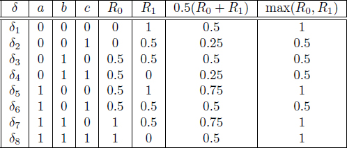
Definition 11.3.1. Bayes Risk Line. For any δ ∈ Δ,

$r\left({\pi }_0;\delta \right)={\pi }_0{R}_0\left(\delta \right)+\left(1-{\pi }_0\right)R_1\left(\delta \right).$

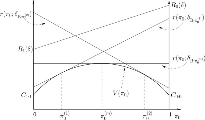
Figure 11.1:  Bayes risk lines and minimum risk curve.

Definition 11.3.2. Bayes Minimum Risk Curve.

$V\left({\pi }_0\right)=\underset{\delta \in \text{Δ}}{\min }r\left({\pi }_0;\delta \right)=r\left({\pi }_0;{\delta }_{\mathrm{B},{\pi }_0}\right),{\pi }_0\in \left[0,1\right]$

where ${\delta }_{\mathrm{B},{\pi }_0}$ is a Bayes rule for prior π₀.

Bayes risk lines and the minimum risk curve are illustrated in Figure 11.1. The following result states some useful properties of V(π₀).

Lemma 11.3.1. V is a concave (continuous) function on [0, 1] with V(0) = C_1,1 and V(1) = C_0,0.

Proof: The minimum of concave functions is concave; therefore, the concavity of V follows from the fact that each of the risk lines r(π₀; δ) is linear (and hence concave) in π₀. As for the end point properties,

$V\left(0\right)=\underset{\delta \in \text{Δ}}{\min }{R}_1\left(\delta \right)=\underset{\delta \in \text{Δ}}{\min }{C}_{0,1}{\mathrm{P}}_1\left({\mathcal{Y}}_0\right)+C_{1,1}{\mathrm{P}}_1\left({\mathcal{Y}}_1\right)=C_{1,1}$

where the minimizing rule is δ*(y) = 1, for all y ∈ $\mathcal{Y}$. Similarly V(1) = C_0,0.

■

We can write V(π₀) in terms of the likelihood ratio L(y) and threshold τ as:

$\begin{array}{l}V\left({\pi }_0\right)={\pi }_0\left[C_{1,0}{\mathrm{P}}_0\left\{L\left(Y\right)\ge \tau \right\}+C_{0,0}{\mathrm{P}}_0\left\{L\left(Y\right)<\tau \right\}\right]\\ +\left(1-{\pi }_0\right)\left[C_{1,1}{\mathrm{P}}_1\left\{L\left(Y\right)\ge \tau \right\}+C_{0,1}{\mathrm{P}}_1\left\{L\left(Y\right)<\tau \right\}\right].\end{array}$

If L(y) has no point masses² under P₀ or P₁, then V is differentiable in π₀ (since τ is differentiable in π₀).

Figure 11.2:  Minimax (equalizer) rule when V is differentiable at ${\pi }_0^{\left(m\right)}$.

11.3.2    Equalizer Rule

Let us first consider the case where V is indeed differentiable for all π₀. Then V(π₀) achieves its maximum value at either the end points π₀ = 0 or π₀ = 1 or within the interior π₀ ∈ (0, 1). If we assume uniform costs, then V(0) = V(1) = 0, and the maximum cannot be attained at the end points. Therefore, we further restrict our analysis to the case of uniform costs (the more general setting is considered in [2]).

Theorem 11.3.1. If C_0,0 = C_1,1 = 0 and V is differentiable on [0, 1], then

${\delta }_m={\delta }_{B,{\pi }_0^m}$

where ${\pi }_0^m=\arg {\max }_{{\pi }_0}V\left({\pi }_0\right)$, obtained by solving dV (π₀)/dπ₀ = 0, i.e., δ_m is a Bayes rule for the worst case prior. Furthermore, δ_m is a Bayes equalizer rule, i.e., R₀(δ_m) = R₁(δ_m). Note that randomization cannot improve the minimax rule in this case.

Proof: The proof follows from Figure 11.2 using the following steps:

1.  For any δ ∈ Δ, the risk line r(π₀; δ) cannot intersect with V(π₀).

2.  For fixed ${\pi }_0^{\left(1\right)}$, the risk line $r\left({\pi }_0;{\delta }_{\mathrm{B},{\pi }_0^{\left(1\right)}}\right)$ is tangent to V at $\pi ={\pi }_0^{\left(1\right)}$.

3.  Any rule with risk line that is not tangential to V cannot be minimax because one can always find a rule with risk line that has the same slope and is tangential to V with smaller R_max.

4.  Among all Bayes rules, the one that has R₀ = R₁ is minimax.

Figure 11.3:  Minimax rule when V is not differentiable at ${\pi }_0^{\left(m\right)}$.

Since the tangent to V at any fixed prior π₀ is unique and corresponds to a deterministic Bayes rule for that prior, randomization cannot yield a better minimax rule.

■

If V is not differentiable for all π₀, then the arguments given in the proof of Theorem 11.3.1 can still be used as long as V is differentiable at its maximum, and the minimax rule is still the unique Bayes rule for the worst case prior. If V is not differential at its maximum, then we have the scenario depicted in Figure 11.3. Note that δ⁻ and δ⁺ are deterministic Bayes rules with same Bayes risk $V\left({\pi }_0^{\mathrm{m}}\right)$, and since they are likelihood ratio tests with δ⁻ having a larger risk under P₀,

${\delta }^{-}=\{\begin{array}{lll}1\hfill & \mathrm{if}\hfill & L\left(y\right)\ge \tau \left({\pi }_0^{\mathrm{m}}\right)\hfill \\ 0\hfill & \mathrm{if}\hfill & L\left(y\right)<\tau \left({\pi }_0^{\mathrm{m}}\right)\hfill \end{array},{\delta }^{+}=\{\begin{array}{lll}1\hfill & \mathrm{if}\hfill & L\left(y\right)>\tau \left({\pi }_0^{\mathrm{m}}\right)\hfill \\ 0\hfill & \mathrm{if}\hfill & L\left(y\right)\le \tau \left({\pi }_0^{\mathrm{m}}\right)\hfill \end{array}$

where $\tau \left({\pi }_0^{\mathrm{m}}\right)={\pi }_0^{\mathrm{m}}/\left(1-{\pi }_0^{\mathrm{m}}\right)$. For δ⁻ and δ⁺ to be different, L(Y) must have a point mass at $\tau \left({\pi }_0^{\mathrm{m}}\right)$, i.e., ${\mathrm{P}}_j\left\{L\left(Y\right)=\tau \left({\pi }_0^{\mathrm{m}}\right)\right\}\ne 0$, for j = 0, 1. This also implies that V is not differentiable at ${\pi }_0^{\mathrm{m}}$. Also, if δ⁻ and δ⁺ are different, then neither of them can be an equalizer rule.

Finding the minimax rule within the set of deterministic rules Δ is challenging in this case, since step 2 in the proof of Theorem 11.3.1 does not hold, and it is possible for a rule that has risk line that is not tangential to V to be minimax within Δ. We may need to resort to brute force enumeration to find minimax rules within Δ as we did in Example 11.1.2. Fortunately we can circumvent this problem by allowing for randomized decision rules.

It should be clear from Figure 11.3 that if an equalizer rule exists in Δ̃, which is tangential to V at ${\pi }_0^{\mathrm{m}}$, then it must be minimax within the class Δ̃. Now, consider

${\tilde{\delta }}_{\mathrm{B},{\pi }_0^{\mathrm{m}}}=\{\begin{array}{ll}{\delta }^{-}\hfill & \mathrm{with}\mathrm{probability}q\hfill \\ {\delta }^{+}\hfill & \mathrm{with}\mathrm{probability}\left(1-q\right)\hfill \end{array}$

The conditional risks of this randomized decision rule are given by

$\begin{array}{l}{R}_0\left({\tilde{\delta }}_{\mathrm{B},{\pi }_0^{\mathrm{m}}}\right)=q{R}_0\left({\delta }^{-}\right)+\left(1-q\right)R_0\left({\delta }^{+}\right)\\ R_1\left({\tilde{\delta }}_{\mathrm{B},{\pi }_0^{\mathrm{m}}}\right)=q{R}_1\left({\delta }^{-}\right)+\left(1-q\right)R_1\left({\delta }^{+}\right)\end{array}$

Thus, setting

$q=\frac{R_1\left({\delta }^{+}\right)-R_0\left({\delta }^{+}\right)}{\left(R_1\left({\delta }^{+}\right)-R_0\left({\delta }^{+}\right)\right)+\left(R_0\left({\delta }^{-}\right)-R_1\left({\delta }^{-}\right)\right)}\triangleq q_m$

(11.14)

produces an equalizer rule.

Theorem 11.3.2. If C_0,0 = C_1,1 = 0 and V is not differentiable at its maximum, then the minimax solution within the set of randomized decision rules Δ̃ is given by the equalizer rule:

${\tilde{\delta }}_m={\tilde{\delta }}_{B,{\pi }_0^m}=\{\begin{array}{lll}1\hfill & if\hfill & L\left(y\right)>\tau \left({\pi }_0^m\right)\hfill \\ 1\mathrm{w}.\mathrm{p}.q_m\hfill & if\hfill & L\left(y\right)=\tau \left({\pi }_0^m\right)\hfill \\ 0\hfill & if\hfill & L\left(y\right)<\tau \left({\pi }_0^m\right)\hfill \end{array}$

where ${\pi }_0^m=\arg {\max }_{{\pi }_0}V\left({\pi }_0\right)$ and q_m is given in (11.14).

11.3.3    Examples

Example 11.3.1. Signal Detection in Gaussian Noise (continued). In this example we study the minimax solution to the detection problem described in Example 11.2.1. We assume uniform costs. We can compute the minimum Bayes risk curve as:

$\begin{array}{l}V\left({\pi }_0\right)={\pi }_0{\mathrm{P}}_0\left\{Y\ge {\tau }^{\prime }\right\}+\left(1-{\pi }_0\right){\mathrm{P}}_1\left\{Y<{\tau }^{\prime }\right\}\\ ={\pi }_{0}Q\left(\frac{{\tau }^{\prime }-{\mu }_0}{\sigma }\right)+\left(1-{\pi }_0\right)\text{Φ}\left(\frac{{\tau }^{\prime }-{\mu }_1}{\sigma }\right)\end{array}$

with

${\tau }^{\prime }=\frac{{\sigma }^2}{{\mu }_1-{\mu }_0}\log \left(\frac{{\pi }_0}{1-{\pi }_0}\right)+\frac{{\mu }_1+{\mu }_0}{2}.$

Clearly V is a differentiable function, and therefore the deterministic equalizer rule is minimax. We can solve for the equalizer rule without explicitly maximizing V. In particular, if we denote the LRT with threshold τ′ (see (11.12)) by δ_τ′, then

$R_0\left({\delta }_{{\tau }^{\prime }}\right)=Q\left(\frac{{\tau }^{\prime }-{\mu }_0}{\sigma }\right),R_1\left({\delta }_{{\tau }^{\prime }}\right)=\text{Φ}\left(\frac{{\tau }^{\prime }-{\mu }_1}{\sigma }\right)=Q\left(\frac{{\mu }_1-{\tau }^{\prime }}{\sigma }\right).$

Setting R₀(δ_τ′) = R₁(δ_τ′) yields

${{\tau }^{\prime }}_{\mathrm{m}}=\frac{{\mu }_1+{\mu }_0}{2}$

from which we can conclude that τ_m = 1 and ${\pi }_0^{\mathrm{m}}=0.5$.

Thus the minimax decision rule is given by

${\delta }_{\mathrm{m}}={\delta }_{\mathrm{B},0.5}=\{\begin{array}{cc}1& \mathrm{if}y\ge \frac{{\mu }_1+{\mu }_0}{2}\\ 0& \mathrm{otherwise}\end{array}$

and the minimax risk is given by

$r\left({\delta }_{\mathrm{m}}\right)=V\left(0.5\right)=Q\left(\frac{{\mu }_1-{\mu }_0}{2\sigma }\right).$

□

Example 11.3.2. Discrete Observations (continued). In this example, we study the minimax solution to the detection problem described in Example 11.2.2. Recall that L(a) = 0, L(b) = 1, and L(c) = ∞. Assuming uniform costs, Bayes rules for prior π₀ (randomized and deterministic) are given by:

${\tilde{\delta }}_{\mathrm{B},{\pi }_0}\left(y\right)=\{\begin{array}{lll}1\hfill & \mathrm{if}\hfill & L\left(y\right)>\tau \left({\pi }_0\right)\hfill \\ 1\mathrm{w}.\mathrm{p}.q\hfill & \mathrm{if}\hfill & L\left(y\right)=\tau \left({\pi }_0\right)\hfill \\ 0\hfill & \mathrm{if}\hfill & L\left(y\right)<\tau \left({\pi }_0\right)\hfill \end{array}$

(11.15)

where τ(π₀) = π₀/(1 − π₀) and q ∈ [0, 1].

For π₀ ∈ (0, 0.5), τ(π₀) ∈ (0, 1), and thus all the Bayes rules in (11.15) collapse to the single deterministic rule:

${\delta }^{-}\left(y\right)=\{\begin{array}{lll}1\hfill & \mathrm{if}\hfill & y=b,c\hfill \\ 0\hfill & \mathrm{if}\hfill & y=a\hfill \end{array}.$

Similarly, for π₀ ∈ (0.5, 1), τ(π₀) ∈ (1, ∞), and thus all the Bayes rules in (11.15) collapse to the single deterministic rule:

${\delta }^{+}\left(y\right)=\{\begin{array}{lll}1\hfill & \mathrm{if}\hfill & y=c\hfill \\ 0\hfill & \mathrm{if}\hfill & y=a,b\hfill \end{array}.$

For π₀ = 0.5, the following set of randomized decision rules are all Bayes rules:

${\tilde{\delta }}_{\mathrm{B},0.5}\left(y\right)=\{\begin{array}{lll}1\hfill & \mathrm{if}\hfill & y=c\hfill \\ 1\mathrm{w}.\mathrm{p}.q\hfill & \mathrm{if}\hfill & y=b\hfill \\ 0\hfill & \mathrm{if}\hfill & y=a\hfill \end{array}$

Figure 11.4:  Minimax rule for Example 11.3.2.

and these rules can be obtained by randomizing between δ⁺ and δ⁻. From the above discussion it is clear that the minimum Bayes risk curve V is as shown in Figure 11.4, with the worst case prior ${\pi }_0^{\mathrm{m}}=0.5$. Furthermore, it is easy to check that R₁(δ⁻) = R₀(δ⁺) = 0, and R₀(δ⁻) = R₁(δ⁺) = 0.5. Therefore, from (11.14), q_m = 0.5, and the minimax decision rule is given by:

${\tilde{\delta }}_{\mathrm{m}}=\{\begin{array}{lll}1\hfill & \mathrm{if}\hfill & y=c\hfill \\ 1\mathrm{w}.\mathrm{p}.0.5\hfill & \mathrm{if}\hfill & y=b\hfill \\ 0\hfill & \mathrm{if}\hfill & y=a\hfill \end{array}$

with minimax risk r(δ̃_m) = V(0.5) = 0.25.

It is interesting to note that δ₂ and δ₄ in Example 11.1.2 are the same as δ⁺ and δ⁻, respectively, and that randomizing between these rules with equal probability is indeed the minimax solution within Δ̃.

□

11.4    Binary Neyman-Pearson Detection

For binary detection problems without a prior on the state, a commonly used alternative to minimax formulation is the Neyman-Pearson formulation, which is based on trading off the following two types of error probabilities:

$\begin{array}{l}\mathrm{P}\mathrm{robability}\mathrm{of}\mathrm{False}\mathrm{Alarm}\triangleq {\mathrm{P}}_{\mathrm{F}}\left(\tilde{\delta }\right)={\mathrm{P}}_0\left\{\tilde{\delta }\left(Y\right)=1\right\}\\ \mathrm{P}\mathrm{robability}\mathrm{of}\mathrm{Miss}\triangleq {\mathrm{P}}_{\mathrm{M}}\left(\tilde{\delta }\right)={\mathrm{P}}_1\left\{\tilde{\delta }\left(Y\right)=0\right\}\end{array}$

(11.16)

The goal is to minimize P_M subject to the constraint P_F ≤ α, for α ∈ (0, 1).

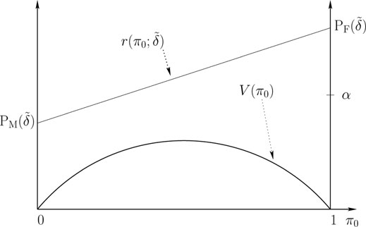
Figure 11.5:  Risk line and Bayesian minimum risk curve for uniform costs.

An alternative measure of performance that is commonly used in radar and surveillance applications is:

$\mathrm{P}\mathrm{robability}\mathrm{of}\mathrm{Detection}\triangleq {\mathrm{P}}_{\mathrm{D}}\left(\tilde{\delta }\right)={\mathrm{P}}_1\left\{\tilde{\delta }\left(Y\right)=1\right\}=1-{\mathrm{P}}_{\mathrm{M}}\left(\tilde{\delta }\right).$

P_D(δ̃) is also called the power of the decision rule δ̃. The Neyman-Pearson (N-P) problem is generally stated in terms P_D and P_F as:

${\tilde{\delta }}_{\text{NP}} = \arg \underset{\begin{array}{l}\tilde{\delta }\in \tilde{\Delta }:\\ {\text{P}}_{\text{F}}(\tilde{\delta })\le \alpha \end{array}}{\max }{\text{P}}_{\text{D}}(\tilde{\delta })\text{for}\alpha \in (0,1).$

(11.17)

Note that unlike the Bayesian and minimax optimization problems, which are formulated in terms of conditional risks, the N-P optimization problem is stated in terms of conditional error probabilities. In particular, we are implicitly assuming uniform costs, which means P_D(δ̃) = 1 ‒ R₁(δ̃) and P_F(δ̃) = R₀(δ̃), and the N-P optimization is to minimize R₁(δ̃) subject to R₀(δ̃) ≤ α.

11.4.1    Solution to the N-P Optimization Problem

To solve the N-P optimization problem, we once again resort to Bayesian risk lines and the minimum risk curve V(π₀) with uniform costs. As depicted in Figure 11.5, the risk line r(π₀; δ̃) for any rule δ̃ ∈ Δ̃ lies above the concave function V(π₀), and intersects the π₀ = 0 line at level P_M(δ̃) and the π₀ = 1 line at level P_F(δ̃). Among all decision rules with risk lines that have intersection with the π₀ = 1 line at a level less than or equal to α, we are interested in the one which has the smallest intersection with the π₀ = 0 line. As in the solution to the minimax problem, let us first consider the case where V is differentiable for all π₀. Then it is clear that the decision rule that solves the N-P problem has a risk line that is tangential to V and intersects the π₀ = 1 line at a level exactly equal to α. Such a rule is deterministic Bayes rule (LRT) that compares the likelihood ratio L(y) to a threshold η that satisfies the P_F constraint.

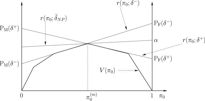
Figure 11.6:  N-P optimization when V is not differentiable for all π₀ ∈ [0, 1].

Theorem 11.4.1. if V is differentiable on [0, 1], then

${\tilde{\delta }}_{NP}\left(y\right)={\delta }_{\eta }=\{\begin{array}{cc}1& ifL\left(y\right)\ge \eta \\ 0& otherwise\end{array}$

where η is chosen so that P₀{L(Y) ≥ η} = α.

Now consider the case where V is not differentiable, and we have the scenario depicted in Figure 11.6. The decision rule δ⁺ is the deterministic LRT that has the largest value of P_F satisfying the constraint P_F ≤ α, and the decision rule δ⁻ is the other deterministic LRT for the same prior. By randomizing between δ⁺ and δ⁻ we can produce a decision rule that has P_F = α, and is hence a solution to (11.17).

Theorem 11.4.2. If V is not differentiable for all π₀ ∈ [0, 1], then

${\tilde{\delta }}_{NP}\left(y\right)={\tilde{\delta }}_{\eta ,\gamma }=\{\begin{array}{lll}1\hfill & if\hfill & L\left(y\right)>\eta \hfill \\ 1\mathrm{w}.\mathrm{p}.\gamma \hfill & if\hfill & L\left(y\right)=\eta \hfill \\ 0\hfill & if\hfill & L\left(y\right)<\eta \hfill \end{array}$

where η and γ are chosen so that P₀{L(Y) > η} + γP₀{L(Y) = η} = α.

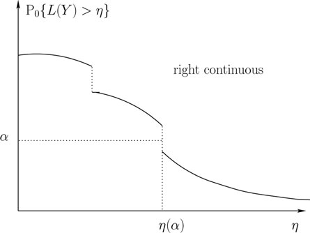
Figure 11.7:  Complementary CDF of the likelihood ratio L(Y).

11.4.2    N-P Rule and Receiver Operating Characteristic

The procedure for finding the parameters η and γ of the Neyman-Pearson solution is illustrated in Figure 11.7, where we plot P₀{L(y) > η} as a function of η. As seen in Figure 11.7, P₀{L(y) > η} is a right continuous function of η. Given P_F constraint α, we first choose η(α) as:

$\eta \left(\alpha \right)=\min \left\{\eta \ge 0:{\mathrm{P}}_0\left\{L\left(y\right)>\eta \right\}\le \alpha \right\}.$

If P₀{L(y) > η(α)} = α, then we do not need to randomize and we can set γ(α) = 0. If P₀{L(y) > η(α)} < α, then we pick γ(α) so that

$\alpha ={\mathrm{P}}_0\left\{L\left(y\right)>\eta \left(\alpha \right)\right\}+\gamma \left(\alpha \right){\mathrm{P}}_0\left\{L\left(y\right)=\eta \left(\alpha \right)\right\}$

which implies that

$\gamma \left(\alpha \right)=\frac{\alpha -{\mathrm{P}}_0\left\{L\left(y\right)>\eta \left(\alpha \right)\right\}}{{\mathrm{P}}_0\left\{L\left(y\right)=\eta \left(\alpha \right)\right\}}$

The probability of detection (power) of δ̃_NP for P_F level α can be computed as:

${\mathrm{P}}_{\mathrm{D}}\left({\tilde{\delta }}_{\mathrm{NP}}\right)={\mathrm{P}}_1\left\{L\left(y\right)>\eta \left(\alpha \right)\right\}+\gamma \left(\alpha \right){\mathrm{P}}_1\left\{L\left(y\right)=\eta \left(\alpha \right)\right\}.$

A plot of P_D(δ̃_NP) versus P_F(δ̃_NP) = α is called the receiver operating characteristics (ROC) of the Neyman-Pearson decision rule (see Figure 11.8). Some properties of the ROC are discussed in Exercise 11. In particular, the ROC is a concave function that lies above the 45° line, i.e., P_D(δ̃_NP) ≥ P_F(δ̃_NP).

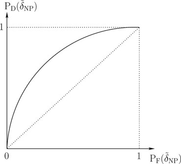
Figure 11.8:  Receiver operating characteristic (ROC).

11.4.3    Examples

Example 11.4.1. Signal Detection in Gaussian Noise (continued). In this example we study the N-P solution to the detection problem described in Example 11.2.1. As in the Bayesian setting of this problem, we can simplify the form of the LRT by noting that

$L\left(y\right)\eta \iff y>{\eta }^{\prime }=\frac{{\sigma }^2}{{\mu }_1-{\mu }_0}\log \eta +\frac{{\mu }_1+{\mu }_0}{2}$

Thus

${\tilde{\delta }}_{\mathrm{NP}}\left(y\right)=\{\begin{array}{lll}1\hfill & \mathrm{if}\hfill & y>{\eta }^{\prime }\hfill \\ 1\mathrm{w}.\mathrm{p}.\gamma \hfill & \mathrm{if}\hfill & y={\eta }^{\prime }\hfill \\ 0\hfill & \mathrm{if}\hfill & y<{\eta }^{\prime }\hfill \end{array}.$

Randomization is not needed since P₀{Y = η′} = P₁{Y = η′} = 0 for all η′ ∈ ℝ, and therefore

${\tilde{\delta }}_{\mathrm{NP}}\left(y\right)={\delta }_{{\eta }^{\prime }}\left(y\right)\{\begin{array}{lll}1\hfill & \mathrm{if}\hfill & y\ge {\eta }^{\prime }\hfill \\ 0\hfill & \mathrm{if}\hfill & y<{\eta }^{\prime }\hfill \end{array}.$

Now

${\mathrm{P}}_{\mathrm{F}}\left({\delta }_{{\eta }^{\prime }}\right)={\mathrm{P}}_0\left\{Y\ge {\eta }^{\prime }\right\}=Q\left(\frac{{\eta }^{\prime }-{\mu }_0}{\sigma }\right).$

Therefore, we can meet a P_F constraint of α by setting

${\eta }^{\prime }\left(\alpha \right)=\sigma Q^{-1}\left(\alpha \right)+{\mu }_0.$

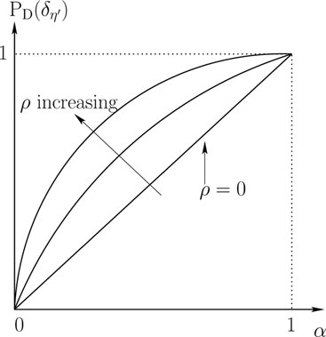
Figure 11.9:  ROC for Example 11.4.1.

The power of δ_η′ is given by:

${\mathrm{P}}_{\mathrm{D}}\left({\delta }_{{\eta }^{\prime }}\right)={\mathrm{P}}_1\left\{Y\ge {\eta }^{\prime }\right\}=Q\left(\frac{{\eta }^{\prime }\left(\alpha \right)-{\mu }_1}{\sigma }\right)=Q\left(Q^{-1}\left(\alpha \right)-\rho \right)$

where ρ = (μ₁ − μ₀)/σ is a measure of the signal–to–noise ratio (SNR). The ROC is plotted in Figure 11.9. As ρ increases, the P_D increases for a given level of P_F.

□

Example 11.4.2. Discrete Observations (continued). In this example we study the N-P solution to the detection problem described in Example 11.2.2. Due to the fact that L(a) = 0, L(b) = 1, and L(c) = ∞, we have that

${\mathrm{P}}_0\left\{L(Y>\eta \right\}=\{\begin{array}{lll}0.5\hfill & \mathrm{if}\hfill & \eta \in [0,1)\hfill \\ 0\hfill & \mathrm{if}\hfill & \eta \in [1,\infty )\hfill \end{array}.$

Thus, for α ∈ (0, 0.5), η(α) = 1 and $\gamma \left(\alpha \right)=\frac{\alpha -0}{0.5}=2\alpha$, which yields

${\tilde{\delta }}_{\mathrm{NP}}\left(y\right)=\{\begin{array}{lll}1\hfill & \mathrm{if}\hfill & y=c\hfill \\ 1\mathrm{w}.\mathrm{p}.2\alpha \hfill & \mathrm{if}\hfill & y=b\hfill \\ 0\hfill & \mathrm{if}\hfill & y=a\hfill \end{array}$

and

${\mathrm{P}}_{\mathrm{D}}\left({\tilde{\delta }}_{\mathrm{NP}}\right)=p_1\left(c\right)+2\alpha p_1\left(b\right)=0.5+\alpha .$

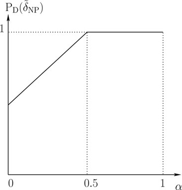
Figure 11.10:  ROC for Example 11.4.2.

For α ∈ [0.5, 1), η(α) = 0 and $\gamma \left(\alpha \right)=\frac{\alpha -0.5}{0.5}=2\alpha -1$, which yields

${\tilde{\delta }}_{\mathrm{NP}}\left(y\right)=\{\begin{array}{cc}1& \mathrm{if}y=c,b\\ 1\mathrm{w}.\mathrm{p}.2\alpha -1& \mathrm{if}y=a\end{array}$

and P_D(δ̃_NP) = 1. The ROC is plotted in Figure 11.10.

□

11.5    Bayesian Composite Detection

So far we have assumed that conditional densities p₀ and p₁ are specified completely. Under this assumption, we saw that all three formulations of the binary detection problem (Bayes, minimax, Neyman-Pearson) led to the same solution structure, LRT, which is a comparison of the likelihood ratio L(y) to an appropriately chosen threshold. We now study the situation where p₀ and p₁ are not specified explicitly, but we are told that they come from a parametrized family of densities {p_θ, θ ∈ Λ}, with Λ being a discrete set or a subset of a Euclidean space. The hypothesis H_j corresponds to θ ∈ Λ_j, j = 0, 1, and Λ₀ ∪ Λ₁ = Λ, Λ₀ ∩ Λ₁ = $\cancel{0}$.

We can consider composite binary detection (hypothesis testing) as a statistical decision theory problem where the set of states $\mathcal{S}$ = Λ is nonbinary, but the set of decisions $\mathcal{D}$ = {0, 1} is still binary, and the cost function relating the decisions and states is of the form:

$C\left(i,\theta \right)=C_{i,j}\mathrm{for}all\theta \in {\text{Λ}}_j,i,j=0,1.$

(11.18)

In this section we consider a Bayesian formulation of the problem, where we assume that the state θ is a realization of a random variable Θ with prior PDF (PMF) given by π(θ). From (11.8), we immediately have that Bayes rule for composite hypothesis testing is given by:

${\delta }_{\mathrm{B}}\left(y\right)\arg \underset{i\in \mathcal{D}}{\min }C\left(i|y\right)$

where, using the notation introduced in (11.2),

$C\left(i|y\right)={\displaystyle {\int }_{\theta \in \text{Λ}}C\left(i,\theta \right)p\left(\theta |y\right)}\mu \left(d\theta \right),\mathrm{with}p\left(\theta |y\right)=\frac{p_{\theta }\left(y\right)\pi \left(\theta \right)}{p\left(y\right)}.$

Using (11.18), we can expand C(i∣y) as:

$C\left(i|y\right)=C_{i,0}{\displaystyle {\int }_{\theta \in {\text{Λ}}_0}p\left(\theta |y\right)}\mu \left(d\theta \right)+C_{i,1}{\displaystyle {\int }_{\theta \in {\text{Λ}}_1}p\left(\theta |y\right)}\mu \left(d\theta \right)$

from which we can easily conclude that:

$C\left(1|y\right)\le C\left(0|y\right)\iff \frac{{\displaystyle {\int }_{\theta \in {\text{Λ}}_1}{p}_{\theta }\left(y\right)\pi \left(\theta \right)}\mu \left(d\theta \right)}{{\displaystyle {\int }_{\theta \in {\text{Λ}}_0}{p}_{\theta }\left(y\right)\pi \left(\theta \right)}\mu \left(d\theta \right)}\ge \frac{C_{1,0}-C_{0,0}}{C_{0,1}-C_{1,1}}.$

(11.19)

Now, if we define the priors on the hypotheses as

${\pi }_j\triangleq {\displaystyle {\int }_{\theta \in {\text{Λ}}_j}\pi \left(\theta \right)\mu \left(d\theta \right),j=0,1.}$

(11.20)

and the conditional densities for the hypotheses as

$p\left(y|{\text{Λ}}_j\right)\triangleq \frac{1}{{\pi }_j}{\displaystyle {\int }_{\theta \in {\text{Λ}}_j}{p}_{\theta }\left(y\right)\pi \left(\theta \right)\mu \left(d\theta \right)}$

then we can see that

$C\left(1|y\right)\le C\left(0|y\right)\iff L\left(y\right)\ge \tau$

with τ as defined in (11.11) and L(y) = p(y∣Λ₁)/p(y∣Λ₀).

Therefore, we can conclude that Bayes rule for composite detection is nothing but a LRT for the (simple) binary detection problem:

$H_0:Y~p\left(y|{\text{Λ}}_0\right)\mathrm{versus}{H}_1:Y~p\left(y|{\text{Λ}}_1\right)$

with priors π₀ and π₁ as defined in (11.20).

Example 11.5.1. Consider the composite detection problem in which Λ = [0, ∞), Λ₀ = [0, 1), and Λ₁ = [1, ∞), with uniform costs, and

$p_{\theta }\left(y\right)=\theta e^{-\theta y}{\mathbb{I}}_{\left\{y\ge 0\right\},}\pi \left(\theta \right)=e^{-\theta }{\mathbb{I}}_{\left\{\theta \ge 0\right\}}$

where $\mathbb{I}$ is the indicator function. To compute the Bayes rule for this problem, we first compute

${\displaystyle {\int }_{\theta \in {\text{Λ}}_1}{p}_{\theta }\left(y\right)\pi \left(\theta \right)\mu \left(d\theta \right)}={\displaystyle {\int }_1^{\infty }\theta e^{-\theta \left(y+1\right)}}d\theta =\frac{\left(y+2\right)e^{-\left(y+1\right)}}{{\left(y+1\right)}^2}$

and

${\displaystyle {\int }_{\theta \in {\text{Λ}}_0}{p}_{\theta }\left(y\right)\pi \left(\theta \right)\mu \left(d\theta \right)}={\displaystyle {\int }_0^1\theta e^{-\theta \left(y+1\right)}}d\theta =\frac{1-\left(y+2\right)e^{-\left(y+1\right)}}{{\left(y+1\right)}^2}.$

Then, from (11.19), we get that

${\delta }_{\mathrm{B}}=\{\begin{array}{ll}1\hfill & \mathrm{if}\left(y+2\right)\ge 0.5e^{\left(y+1\right)}\hfill \\ 0\hfill & \text{otherwise}\hfill \end{array}$

which can be simplified to

${\delta }_{\mathrm{B}}=\{\begin{array}{ll}1\hfill & \mathrm{if}0\le y\le {\tau }^{\prime }\hfill \\ 0\hfill & \mathrm{if}y>{\tau }^{\prime }\hfill \end{array}$

where τ′ is a solution to the transcendental equation (y + 2) = 0.5e^(y+1).

□

11.6    Neyman-Pearson Composite Detection

We now consider the more interesting setting for the composite detection problem where there is no prior on the state. A common way to pose the optimization problem in this setting is a generalization of the Neyman-Pearson formulation (see (11.16)). We define the probabilities of false alarm and detection of a test δ̃ ∈ Δ̃ by:

$\begin{array}{l}{\mathrm{P}}_{\mathrm{F}}\left(\tilde{\delta };\theta \right)={\mathrm{P}}_{\theta }\left\{\tilde{\delta }\left(Y\right)=1\right\},\theta \in {\text{Λ}}_0\\ {\mathrm{P}}_{\mathrm{D}}\left(\tilde{\delta };\theta \right)={\mathrm{P}}_1\left\{\tilde{\delta }\left(Y\right)=1\right\},\theta \in {\text{Λ}}_1\end{array}$

The goal in UMP detection is to constrain P_F(δ̃; θ) ≤ α, for all θ ∈ Λ₀, and to simultaneously maximize P_D(δ̃; θ), for all θ ∈ Λ₁. If such a test exists, it is called UMP.

11.6.1    UMP Detection with One Composite Hypothesis

We begin by studying the special case where only H₁ is composite, i.e., Λ₀ is the singleton set equal to {θ₀}. The UMP optimization problem can be stated as:

$\mathrm{Maximize}{\mathrm{P}}_{\mathrm{D}}\left(\tilde{\delta };\theta \right),\mathrm{for}\mathrm{all}\theta \in {\text{Λ}}_1,\mathrm{subject}\mathrm{to}{\mathrm{P}}_{\mathrm{F}}\left(\tilde{\delta };{\theta }_0\right)\le \alpha .$

For fixed θ₁ ∈ Λ₁, we can compute the likelihood ratio as

$L_{{\theta }_1}\left(y\right)=\frac{p_{{\theta }_1}\left(y\right)}{p_{{\theta }_0}\left(y\right)}$

and the corresponding Neyman-Pearson test is given by (see Theorem 11.4.2)

${\tilde{\delta }}_{\mathrm{NP}}\left(y;{\theta }_1\right)=\{\begin{array}{lll}1\hfill & \mathrm{if}\hfill & L_{{\theta }_1}\left(y\right)>{\eta }_{\alpha }\left({\theta }_1\right)\hfill \\ 1\mathrm{w}.\mathrm{p}.{\gamma }_{\alpha }\left({\theta }_1\right)\hfill & \mathrm{if}\hfill & L_{{\theta }_1}\left(y\right)={\eta }_{\alpha }\left({\theta }_1\right)\hfill \\ 0\hfill & \mathrm{if}\hfill & L_{{\theta }_1}\left(y\right)<{\eta }_{\alpha }\left({\theta }_1\right)\hfill \end{array}$

with γ_α(θ₁) and γ_α(θ₁) satisfying

${\mathrm{P}}_{{\theta }_0}\left\{L\left(Y\right)>{\eta }_{\alpha }\left({\theta }_1\right)\right\}+{\gamma }_{\alpha }\left({\theta }_1\right){\mathrm{P}}_{{\theta }_0}\left\{L\left(Y\right)={\eta }_{\alpha }\left({\theta }_1\right)\right\}=\alpha .$

Now, if it turns out that δ̃_NP(y; θ₁) is independent of θ₁, then that test is UMP since it is the N-P solution for all θ₁ ∈ Λ₁. Otherwise, no UMP solution exists. In the following, we provide some illustrative examples.

Example 11.6.1. Detection of One-Sided Composite Signal in Gaussian Noise. This detection problem arises in communications and radar applications where the signal amplitude is unknown but the phase is known. The two hypotheses are described by:

$H_0:Y=Z\mathrm{versus}{H}_1:Y=\theta +Z$

where θ > 0 is an unknown parameter (signal amplitude), and Z ~ $\mathcal{N}$(0, σ²). This is a composite detection problem with θ₀ = 0, and Λ₁ = (0, ∞).

For fixed θ > 0, L_θ(y) = p_θ(y)/p₀(y) has no point masses under P₀ or P_θ, and therefore δ̃_NP(y; θ) is deterministic LRT:

${\delta }_{\mathrm{NP}}\left(y;\theta \right)=\{\begin{array}{lll}1\hfill & \mathrm{if}\hfill & L_{\theta }\left(y\right)\ge \eta \left(\theta \right)\hfill \\ 0\hfill & \mathrm{if}\hfill & L_{\theta }\left(y\right)<\eta \left(\theta \right)\hfill \end{array}=\{\begin{array}{lll}1\hfill & \mathrm{if}\hfill & y\ge {\eta }^{\prime }\left(\theta \right)\hfill \\ 0\hfill & \mathrm{if}\hfill & y<{\eta }^{\prime }\left(\theta \right)\hfill \end{array}$

where (see Example 11.4.1) η′(θ) is given by

${\eta }^{\prime }\left(\theta \right)=\frac{{\sigma }^2\log \eta \left(\theta \right)}{\theta }+\frac{\theta }{2}.$

For an α-level test we need to find η′_α(θ) such that P₀{Y ≥ η′_α(θ)} = α. Exploiting the fact that Y ~ $\mathcal{N}$(0, σ²) under P₀, we get

$Q\left(\frac{{{\eta }^{\prime }}_{\alpha }\left(\theta \right)}{\sigma }\right)=\alpha \Rightarrow {{\eta }^{\prime }}_{\alpha }\left(\theta \right)=\sigma Q^{-1}\left(\alpha \right).$

Note that η′_α(θ) is independent of θ, and therefore the UMP solution is given by:

${\delta }_{\mathrm{UMP}}=\{\begin{array}{lll}1\hfill & \mathrm{if}\hfill & y\ge \sigma Q^{-1}\left(\alpha \right)\hfill \\ 0\hfill & \mathrm{if}\hfill & y<\sigma Q^{-1}\left(\alpha \right)\hfill \end{array}.$

Note that while the test δ_UMP is independent of the θ, the performance of the test in terms of the P_D depends strongly on θ. In particular,

${\mathrm{P}}_{\mathrm{D}}\left({\delta }_{\mathrm{UMP}};\theta \right)={\mathrm{P}}_{\theta }\left\{Y\ge \sigma Q^{-1}\left(\alpha \right)\right\}=Q\left(Q^{-1}\left(\alpha \right)-\theta /\sigma \right).$

□

Example 11.6.2. Detection of Two-Sided Composite Signal in Gaussian Noise. This detection problem arises in communications and radar applications where the signal amplitude and phase are both unknown. The two hypotheses are as described in Example 11.6.1, except that θ ∈ ℝ, i.e., θ can be both positive and negative. There is no UMP test for this problem. This can be seen as follows.

First consider θ = 1. Then following the same steps as in Example 11.6.1, we can show that the α-level N-P test is given by:

${\delta }_{\mathrm{NP}}\left(y;1\right)=\{\begin{array}{lll}1\hfill & \mathrm{if}\hfill & y\ge \sigma Q^{-1}\left(\alpha \right)\hfill \\ 0\hfill & \mathrm{if}\hfill & y<\sigma Q^{-1}\left(\alpha \right)\hfill \end{array}.$

Now, consider θ = −1. Then, it is not difficult to see that L₋₁(y) ≥ η iff y ≤ η′ in this case. Therefore the α-level N-P test is given by:

${\delta }_{\mathrm{NP}}\left(y;-1\right)=\{\begin{array}{lll}1\hfill & \mathrm{if}\hfill & y\le \sigma {\text{Φ}}^{-1}\left(\alpha \right)\hfill \\ 0\hfill & \mathrm{if}\hfill & y<\sigma {\text{Φ}}^{-1}\left(\alpha \right)\hfill \end{array}.$

Since the most powerful tests for θ = −1 and θ = 1 are not the same, there is no uniformly most powerful test.

Example 11.6.3. Detection of One-Sided Composite Signal in Cauchy Noise. From Examples 11.6.1 and 11.6.2, we may be tempted to conclude that for problems involving signal detection in noise, UMP tests exist as long as H₁ is one-sided. To see that this is not true in general, we consider the example where the noise has a Cauchy distribution, i.e.,

$p_{\theta }\left(y\right)=\frac{1}{\pi \left[1+{\left(y-\theta \right)}^2\right]}$

and we are testing H₀ : θ = 0 against the one-sided composite hypothesis H₁ : θ > 0. Then

$L_{\theta }\left(y\right)=\frac{1+y^2}{1+{\left(y-\theta \right)}^2}.$

It is easy to check that the α-level N-P tests for θ = 1 and θ = 2 are different, and hence there is no UMP solution.

□