7.1 INTRODUCTION
In this chapter we investigate how the liquidity buffer (LB from now on) comes about in the running of the business of a financial institution. In greater detail, we will study:
- when the need to set up a LB arises;
- how the LB is financed;
- how LB costs are charged to banking products.
Hopefully we will clarify some concepts that eventually will assist in the liquidity management and the assignment of costs and/or benefits to the different departments within a financial institution.
7.2 LIQUIDITY BUFFER AND COUNTERBALANCING CAPACITY
It is worth defining the LB and its relationship with counterbalancing capacity (CBC), which is a concept normally used in liquidity management practice, although we have not yet introduced it in our analysis. We should stress the fact that there is not a single definition for both and banks often adopt different criteria to define them.
In general, it is possible to define CBC such as to embed it in the LB as well, hence making it a part of the LB.
Definition 7.2.1 (counterbalancing capacity). CBC is a set of strategies by which a bank can cope with liquidity needs by assuming the maximum possible liquidity generation capacity (LGC).
CBC identifies all the possible strategies to generate positive cash flows to make cumulated cash flows, up to given future date, always greater than or at least equal to zero. Positive cash flows can be generated by contractual redemptions and/or interest payments to the bank: these cash flows are not considered by CBC. In our analysis we link CBC to the concept of LGC we saw in Chapter 6 in the sense that it is the most effective configuration the latter can assume in terms of liquidity potential. In practice and in most of literature the concept of CBC clashes with our LGC: the distinction we made could prove useful but it is not essential and as long as there is agreement on the terms adopted, we can safely interchange them.
We give the description of CBC provided by the EBA in the Guidelines on Liquidity Buffers & Survival Periods [6] since it may help in bringing about a common definition:
…the counterbalancing capacity should be a plan to hold, or have access to, excess liquidity over and above a business-as-usual scenario over the short, medium and long-term time horizons in response to stress scenarios, as well as a plan for further liquidity generation capabilities, whether through tapping additional funding sources, making adjustments to the business, or through other more fundamental measures. The latter element should be addressed through the establishment of contingency funding plans. Counterbalancing capacity, therefore, includes but is much broader than the liquidity buffer.
The liquidity buffer has no precise definition and banks use different notions for it (sometimes the LB is often assimilated into the BSL, but actually the latter mainly coincides with the former as made clear from our definitions in Chapter 6). Since no unique definition exists in practice, we can resort to the definitions contained in the above-mentioned Guidelines on Liquidity Buffers & Survival Periods [6], and define the LB as given in Definition 7.2.2.
Definition 7.2.2 (liquidity buffer). The available liquidity covering the additional need for liquidity that may arise over a defined short period of time under stress conditions.
Moreover, again according to the EBA, the LB should be the short end of CBC, and excess liquidity available outright should be used in liquidity stress situations within a given short-term period, excluding the need to take any extraordinary measures.
There are three features that characterize the LB:
- The size of the buffer, which is determined from the funding gap that arises under stressed conditions. To determine the size we need a framework to design stressed scenarios that would cause the gap.
- The specified time horizon (or survival period) considered: funding gaps falling within this period are covered by the buffer. The survival period is only “the period during which an institution can continue operating without needing to generate additional funds and still meet all its payments due under the assumed stress scenarios” [6].
- Composition of the buffer: not only cash, but also highly liquid unencumbered assets can be constituents of the LB.
The main purpose of the LB is to enable a financial institution to get through liquidity stress during a defined survival period, without changing the business model. In what follows we focus on the LB, because we think it is the most important part of CBC for two reasons: (i) it is essential to guarantee the survival of the bank during liquidity stress, and (ii) it is less dependent on strong changes in business-as-usual activity in the medium to long run, which may turn out to be difficult to identify and subject to a high degree of subjectivity.
Definition of the LB and its relationship with the CBC is important but does not provide practitioners with operative rules determining how big the LB should be, when it should be constituted, the cost to the bank of keeping a buffer within the balance sheet, if and how this cost—if any—should be charged to other assets (or liabilities) and, finally, how the composition of the buffer, in terms of cash and other assets included within it, affects its LGC. In the following sections we investigate all these issues.
7.3 THE FIRST CAUSE OF THE NEED FOR A LIQUIDITY BUFFER: MATURITY MISMATCH
First of all, we need to ascertain the occasions when banking activity generates the need to build a LB.
Proposition 7.3.1. The need for a liquidity buffer is brought about by an investment in an asset whose maturity is longer than the liability used to finance it.
Proposition 7.3.2. The investment in an asset that requires a liquidity buffer determines the term structure of the liquidity available to the bank for investments in other assets as well, according to the following factors:
- the expiry of the asset the bank wants to invest;
- the expiry of the source of liquidity, and hence the number of rollovers needed, to finance the purchase of the asset;
- the size of the funding gap on rollover dates under stressed scenarios.
To prove the propositions, we think the best approach is to analyse the operations of a simplified and stylized bank, from the start of its operations.
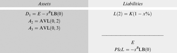
Assume the bank starts at T0 = 0 with an equity equal to E, which is deposited in a bank account D1 yielding no interest; at the same time it issues a (zero-coupon) bond whose present value is K and whose expiry is at T1 = 1: the funds raised are deposited in a bank account D2. For simplicity we assume that is no credit risk in the economy and that the interest rate paid in one period is r for all securities. The balance sheet of the bank at time 0 is the following:
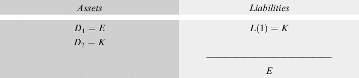
Up to this point there is no need to build a LB: we can devise any stressed scenario, but the bank is perfectly capable to cope with any of it, since its assets are fully liquid, being cash.
Assume now that the bank wants to invest the funds raised to run its major activity: lending money, which is often performed by exploiting one of the expertises of the banking industry (i.e., by maturity transformation). This means that the assets typically have a maturity longer than the liabilities. Let A3 (the asset the bank wants to invest money in) be a loan expiring at T3 = 3. We also assume that equity is not used to finance investments but is just invested in liquidity to cover unexpected losses.
If this is the case, the bank has to decide how much of the funds raised via the bond issuance can be lent, keeping in mind the bond expiry at T1 = 1, so that it has to roll over with an equivalent bond at times T1 = 1 and T2 = 2. If abundant liquidity is available in the market on rollover dates and the bank has no specific problems in the running of its activities, it can be fairly expected that the rollover can easily be operated.
The bank can also design a stressed scenario in which the rollover is difficult for reasons that could be linked to the market (systemic) or to the bank itself (idiosyncratic). Assume in a stressed scenario the bank is not able to roll over a percentage x% of the maturing debt at times 1 and 2. We can think of this percentage as the maximum funding gap that can occur at a given confidence level (say, 99%), similarly to the treatment of the losses suffered for credit or market events on the contracts the bank has in its portfolios.1
At time 0 the available liquidity AVL(0, 3) for the investments can be computed as:
Equation (7.1) states that at each rollover date (there are two of them) the bond's quantity is deducted by x%: this means that the amount of assets expiring at T3 = 3 that can be funded with debt of shorter duration, is only AVL(0, 3) and not K. The difference between the amount raised at 0 via the bond issuance and the AVL(0, 3) is the total liquidity buffer LB(0) = K − AVL(0, 3).
The LB at time T0 = 0 can also be seen as the sum of the two funding gaps FG(1) = x%K and FG(2) = x%K(1 − x%) that may occur under stressed scenarios on rollover dates. It is straightforward to check that:
LB(0) = FG(1) + FG(2) = x%K + x%K(1 − x%) = K − AVL(0, 3)
We can immediately see that the LB, although determined at the start of the activity, can be used in the case of necessity only on the two rollover dates. For all the other dates between time 0 and the second rollover date 2, the LB can be invested, under the constraint that it “exists” in its full liquid form in the amount required when the stressed condition may hurt bank activity.
In our case the available liquidity that can be invested to buy an asset expiring at time 3 is AVL(0, 3); the remaining liquidity needed to build the LB can be invested for an amount x%K in an asset A1 (say, another loan) maturing at time 1, and for an amount x%K(1 − x%) in an asset A2, similar to A1, maturing at time 2. The liquidity generated by asset A1 at its expiry is the amount of the LB in its liquid form that is needed to cope with a stressed scenario on the first rollover date. Analogously the liquidity generated by asset A2 at its expiry is the liquid LB needed to cover the possible funding gap on the second rollover date.
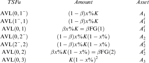
Stressed scenarios and hence the needed liquidity buffer, jointly with the investment in the asset expiring at time T3 = 3, determine the term structure of (available) funding TSFu, defined as:
In the specific case we are examining, TSFu(0, 3) can be summarized as follows:
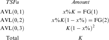
The total is clearly the amount raised by the issuance of bond L. The TSFu is a byproduct of the size of the total LB and is a function of the liquidity gap that can occur on rollover dates (in our modelling, this is the percentage x% of the amount of the bond to be rolled over).
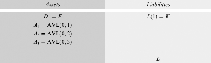
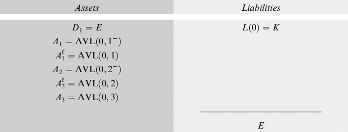
The liquidity available is invested in the three assets, so that at time 0 the balance sheet now reads:
As is immediately apparent, we are trying to build a liquidity buffer in a consistent and sound fashion, strictly linked to the funding of the assets. As such, the LB(0) is build at time 0 to cover funding gaps that may arise in the medium to long term at times 1 and 2, (the periods are likely measured in years in this case). This may appear in stark contrast to Definition 7.2.2, where stressed conditions that need to be covered by the buffer refer to short-term horizons (say, one or two months).
The problem is that, although the LB should be able to cover stressed market condition in the short term, its building and size should be simultaneous with its origination and thus related to a long-term view. What lies behind the need for the LB is the duration mismatch between liabilities and assets, produced by investment of the funds raised. The LB, given the stressed scenarios and the type of the mismatch, can be determined right from the start of the investment. Even if stressed conditions are referred to times far in the future and not to the short term, the approach we outlined is the soundest and most consistent way of setting up a LB to grant financial and liquidity equilibrium in the long term.
The LB can be invested in a risk-free deposit up to the time it is needed to cover potential gaps, or it can be invested in other assets according to the available liquidity schedule we have shown above. In the risk-free economy we are working in at the moment, the two alternatives can be equivalent. The need to have the LB fully liquid in the due amount on rollover dates strictly defines the amount that can be invested in other assets with expiry at times T1 and T2. We will see in the following sections what happens when default risk is introduced.
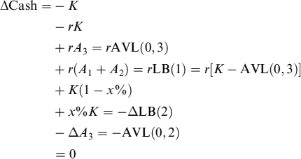
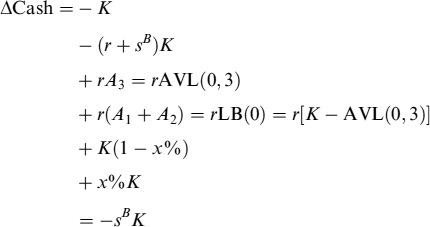
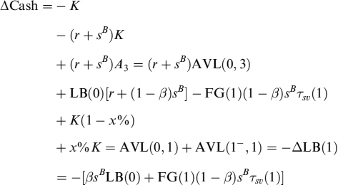
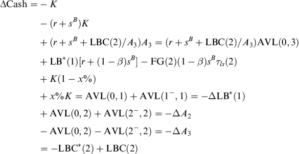
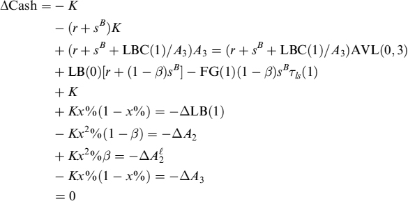
To check whether the LB build at 0 is effective enough to cover future liquidity gaps, we assume that on both rollover dates the stressed scenarios actually happen. Let us see how the activity evolves at time 1: the maturing bond L has to be reimbursed and this can only be done if the bank rolls over the debt for an equivalent amount K. Since the stressed scenario occurs, the actual amount that can be rolled over is only K × (1 − x%); the remaining liquidity necessary to fully pay back the maturing bond, x% × K, is provided by the LB whose liquidity is increased by the maturing asset A1, which is thus correspondingly abated. The total cash variation ΔCash is, keeping in mind the interest the bank pays on the maturing debt and that it receives on the assets and on the LB(0) (invested between time 0 and 1):2
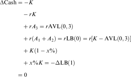
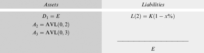
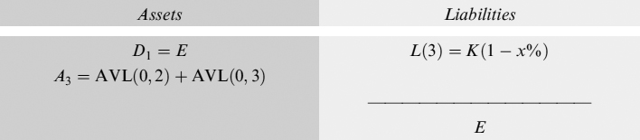
where ΔLB(1) is variation of the liquidity buffer at time T1 = 1. The remaining LB is left invested in asset A2, and the balance sheet is:
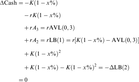
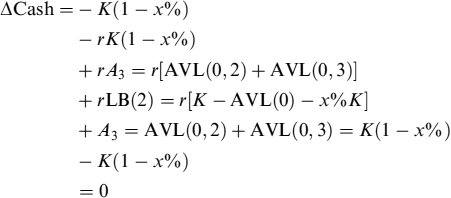
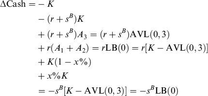
On the rollover date T2 the bank faces the same stressed scenario, so that it has to reimburse the bond L(2) = K(1 − x%), but the funds it can raise are only L(3) = K(1 − x%)2. The difference K(1 − x%) − K(1 − x%)2 has to be drawn from the buffer LB(1) that remains, whose liquidity is produced by the expiring investment in A2 = AVL(0, 2) = K(1 − x%) − K(1 − x%)2. Keeping in mind the interest paid and received, variation of the cash available to the bank is:
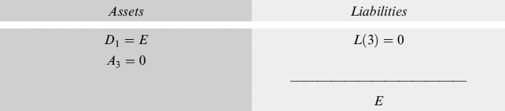
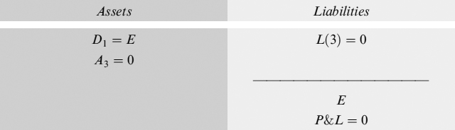
The balance sheet at time T2 = 2 is:
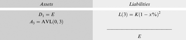
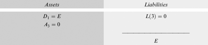
The LB is completely depleted and no longer invested in any asset: this is because it is no longer needed. In fact, at time T3 = 3 the bond L(3) must be reimbursed, requiring a liquidity equal to K(1 − x%)2 that is covered by the expiry of asset A3, implying an equal inflow of AVL(0, 3) = K(1 − x%)2. Keeping in mind the interest paid and received, total cash flow variation is:
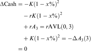
where ΔA3(3) is the variation of asset A3 at time T3 = 3, generating cash for an amount −ΔA3. The balance sheet is:
It is straightforward to check that such a strategy to set up the LB fully covers all possible stress scenarios. Moreover, given the economy we have assumed without credit risk, the total P&L at the end of each period is nil and the LB does not imply any cost that has to be charged over the assets or the liabilities.
7.3.1 Some or all stressed scenarios do not occur
We extend our analysis to the cases when some or all stressed scenarios do not occur. We can prove the following.
Proposition 7.3.3. In an economy with no credit risk, and no funding spread paid by the bank over the risk-free rate, the liquidity buffer does not generate any P&L, either if it is used at any predicted time or if it is not used because the stressed scenario does not manifest (or it manifests in a less disruptive fashion than assumed). Thus there are no costs to be charged (or benefits to be assigned) to assets or liabilities.
Furthermore, we can also verify Proposition 7.3.4.
Proposition 7.3.4. The LB can be set up at the beginning of the investment in an asset, given the assumptions the bank makes about stressed conditions on rollover dates. Moreover, the LB can be reinvested in assets earning the interest rate r (say, loans) as long as these assets mature on the rollover dates or just before them, but never after them.
An immediate consequence is given in Proposition 7.3.5.
Proposition 7.3.5. The setting of a LB, given the assumptions about stressed conditions on rollover dates, also determines the constraints on the maturity transformation rule that a bank can adopt.
If stressed scenarios do not occur, then a profit is produced equal to the interest earned on the investment of the LB in single periods. This profit exactly compensates the greater amount of interest paid by the bank on the issued debt. To clarify this point, assume that at T1 = 1 there is no stressed market or bank-specific condition such that the matured bond can be rolled over for the entire amount. In this case the LB does not have to be utilized and its amount at time T1 = 1 is the same as at time T0 = 0. The liquidity generated by the expiry of asset A1 is invested in asset A2, whose quantity on the balance sheet is increased. The total variation of the cash is:
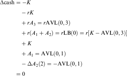
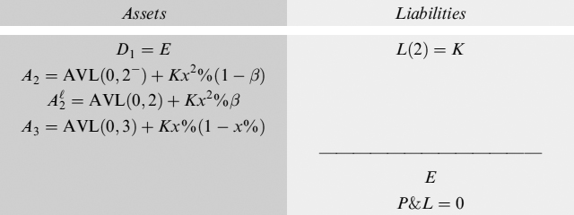
where ΔA2(2) is the cash needed to make the investment in A2 equal to the liquidity generated by the expiry of asset A1. The balance sheet is now:
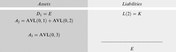
No P&L is generated and the total cash flow is nil. At time T2 = 2 a stressed scenario manifests itself, so the debt can be rolled over only for a fraction of its amount which is equal to (1 − x%); in this case the liquidity buffer is utilized for an amount x%K = AVL(0, 1). The remaining liquidity can be invested in asset A3, whose quantity is correspondingly increased, and we have the following total cash flows:
and the new balance sheet is:
Note the perfect balance between the cash flows and the P&L, which are both still 0. This balanced condition is preserved through to the last period, when we get as total cash flows:
The liquidity needed to reimburse bond L(3) is generated by asset A3 expiring on the same date. The final balance sheet is:
with no P&L generated.
In the analysis just presented, the amount of asset A3 that can be funded by shorter liabilities is determined once funding gaps have been determined for rollover dates. This does not mean that the LB implied by the devised stressed scenarios is the only factor affecting the maturity transformation policy: the constraints set by the liquidity buffer can be tightened by other factors other than the funding gap.
7.3.2 The cost of the liquidity buffer for maturity mismatch
Proposition 7.3.6. In an economy where economic agents (including the bank) can go bankrupt and the bank pays a funding spread over the risk-free rate to remunerate its credit risk, the cost of the liquidity buffer is different from zero and depends on: (i) the level of the funding spread over the risk-free rate paid by the bank, (ii) the bank's preference to invest the buffer in liquid assets traded in the market and (iii) the length of the survival period chosen by the bank.
To prove Proposition 7.3.6, assume that the economy in which the bank operates also embeds default risk: this means that there are economic agents, including the bank, that may go bankrupt. As a consequence, when borrowing money, defaultable agents have to pay a premium over the risk-free rate to compensate the lender for the default risk it bears. From the borrower perspective, this premium is the funding spread and it is a cost it has to consider when evaluating projects within its business activity; from the borrower perspective, it is remuneration for expected future losses due to the default of the borrower.3
In such an economy, the bank pays a funding spread sB and can invest in assets subject to default risk, requiring a credit spread sA to match expected future losses. Nevertheless, the expected return on a defaultable asset is actually the risk-free rate in every case. In fact, the credit spread is set so that on maturity of the asset the expected return is the risk-free rate. For example, assuming asset A expires in a single period, we have that:
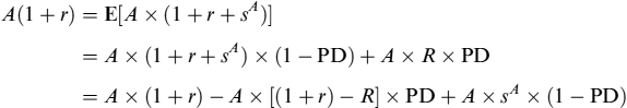
So, the starting value A, accrued at the risk-free interest rate, has to be equal to the initial value compounded at the risk-free rate plus the credit spread, weighted by the probability the counterparty survives (1 − PD) or, alternatively, it is the recovery value A × R, weighted by the probability the counterparty defaults (PD), as shown in the second line. The third line rewrites the expression as the sum of the risk-free asset minus the expected loss (LGD = [(1 + r) − R] is the loss given default, expressed as a fraction of the face value A), plus the credit spread weighted by the survival probability.
The fair credit spread can be derived by solving the above equation, and is:
So the spread is just the loss suffered upon the counterparty's default, weighted by the probability of default (i.e., the expected loss), divided by the survival probability. We can assume that the credit spread is set in such a way that each asset in which the bank invests its funds earns the risk-free rate, on an expected basis, even if its contract rate may be higher.
Let us investigate what happens to the management of the LB in such an environment. We reprise the example we presented in Section 7.3: at the start of activity at T0 = 0 nothing changes in terms of the AVL invested in assets A1, A2 and A3, each one earning the expected risk-free rate r. The LB is built accordingly and the available liquidity at times T1 and T2 is invested in assets earning the (expected) risk-free rate r as well. Let us see which is the total cash flow in T1 = 1:
The liquidity gap is covered by the liquid amount of the buffer produced by the expiry of asset A1. The balance sheet is:
The balance sheet shows the bank suffered a loss at the end of the first period equal to the funding spread (i.e., the spread above the risk-free rate) it has to pay to fund its activity. The loss has been covered by abating the amount of equity deposited in account D1. This is absolutely normal, since we have assumed that the bank invested the funds raised in assets A1, A2, A3 earning the (expected) risk-free rate. The loss is due to the fact that the bank did not charge the funding spread it has to pay on asset A3. Note that this loss has nothing to do with the liquidity buffer used to cope with funding gaps.
A bank usually has strong bargaining power with some counterparties, typically retail customers, and is able to transfer all the costs related to banking activity on an asset bought from them. For example, if asset A3 is a mortgage closed with a retail customer, the bank can charge a spread sA, over the risk-free rate, to compensate the credit risk of the counterparty and a supplementary spread sB to cover its funding costs. So the asset would earn (following the same reasoning as above) an expected return equal to the risk-free rate plus the bank's funding spread:4
E[A3(1 + r + sA + sB)] = A3(1 + r + sB)
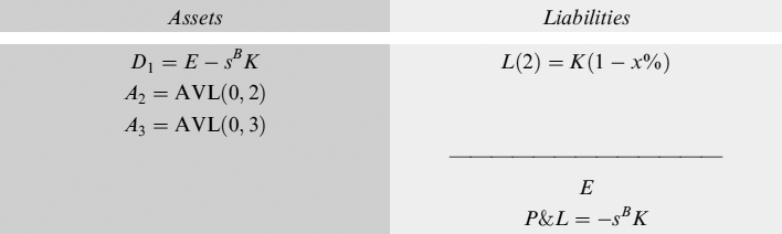
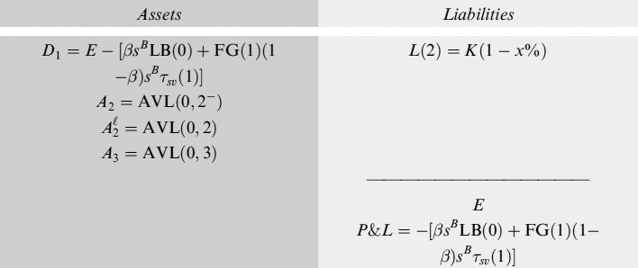
Let us now assume that at time 0 the bank actually closed a mortgage contract charging the funding spread in the contract rate. Assume also that the LB is invested in A1 and A2 which are liquid (almost) risk-free bonds, such as a government bond: on these investments the bank does not have the bargaining power to charge all its costs and must accept the yield set by the market, which we suppose to include remuneration for the credit risk only, so that the expected return is the risk-free rate. Under these assumptions, the total cash flow is:
and the balance sheet is:
The loss is now reduced to −sB LB(0) from −sBK and it is due only to the fact that the bank invested the amount of the liquidity buffer into liquid assets, whose yield had to be accepted as set by the market when they were bought. This loss can be considered a component of the cost of holding the liquidity buffer and consequently has to be charged on the assets that caused a need for the liquidity buffer, in our case asset A3.
Although the constraints relating to the expiry of the investment of the LB have to be satisfied, the bank does not have to necessarily invest the entire amount LB(0) in liquid securities traded in the market for all the following periods. From Definition 7.2.2 the liquidity buffer needs to cover funding gaps within a short survival period, usually taken equal to one month. So, if the period up to the first rollover date is, say, one year, the bank may invest the buffer amount in assets traded with retail customers for 11 months, so that it can charge funding costs as well; then it can invest in liquid securities the amount needed to cover the funding gap of the first rollover date just 1 month before T1 = 1. Similarly, the amount needed for the funding gap on the second rollover date can be invested in assets bought from retail customers up to the start of the survival period before T2.
We can also reasonably assume that, given the risk aversion of the bank, a fraction β is invested in liquid marketable securities in any case, and only a fraction 1 − β is invested in less liquid assets dealt with retail customers. Parameter β can be considered a preference for liquid investment.
Given these assumptions, we first need to determine the new TSFu and the assets in which the available liquidity can be invested. Let us introduce two more assets, ![]() and
and ![]() , representing liquid securities actively traded in the market and maturing, respectively, at times T1 = 1 and T2 = 2. Moreover, let τsv be the survival period chosen by the bank, and let
, representing liquid securities actively traded in the market and maturing, respectively, at times T1 = 1 and T2 = 2. Moreover, let τsv be the survival period chosen by the bank, and let ![]() and
and ![]() be the times before the rollover dates given the length of the survival period. The TSFu is:
be the times before the rollover dates given the length of the survival period. The TSFu is:
where, with a slight abuse of notation, we indicate ![]() and similarly for the other rollover dates. It is worthy of note that, during the period between 0 and the start of the survival period [0, 1−], the amount A1 + A2 = (1 − β)LB(0) is invested in less liquid assets; on the other hand, over the entire first period [0, 1], the amount
and similarly for the other rollover dates. It is worthy of note that, during the period between 0 and the start of the survival period [0, 1−], the amount A1 + A2 = (1 − β)LB(0) is invested in less liquid assets; on the other hand, over the entire first period [0, 1], the amount ![]() is invested in liquid securities traded in the market; during the first survival period [1−, 1],
is invested in liquid securities traded in the market; during the first survival period [1−, 1], ![]() .
.
The balance sheet at time 0 is then modified as follows:
The cost of the liquidity buffer is getting more complicated to compute, but it is not a difficult task. In fact, assuming for simplicity's sake5 that the credit risk of all marketable assets is the same and compensated by a spread sY, whereas the credit spread for all other assets is sA, the LB earns the following return in the first period before the rollover date T1:
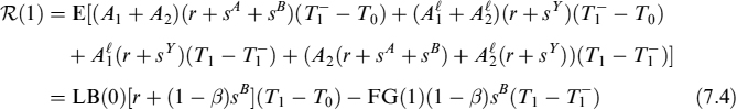
It is worth pointing out the constituent parts of equation (7.4):
- The first line of the equation indicates the fraction (1 − β) invested in the less liquid assets A1 and A2 earning the risk-free rate plus the credit and the bank's funding spread, for a period between time T0 and the time of the start of the first survival period
 . The complementary fraction β is invested in the same period in marketable securities
  earning the risk-free rate plus the credit spread.
 - In the second line, for the remaining period
 (i.e., the first survival period), an amount equal to the funding gap FG(1) is invested in liquid asset
  , earning the risk-free rate plus the credit spread; the remaining part of the liquidity buffer LB(0) is invested in illiquid asset A2 (whose return includes the bank's funding spread) and liquid asset
  (with a return equal to the risk-free rate plus the credit spread).
 - The third line shows the return from the buffer by computing the expectations and by rearranging terms in a more convenient and clear fashion. Basically, the return from the LB is equal, over the entire [T0, T1], to the risk-free rate for the full amount, plus the bank's funding spread for the fraction 1 − β. This is given by the first part of the third line, which does not consider the fact that, during the survival period
 , a share of the LB equal to the funding gap on the first rollover date, FG(1), is diverted to investment in liquid assets, so that the return equal to the bank's funding spread on this amount has to be deducted from the total return: this is given by the second part of the third line.
To lighten the notation, we can denote the entire first period by τ(1) = T1 − T0, and the survival period by ![]() . Equation (7.4) can then be rewritten as:
. Equation (7.4) can then be rewritten as:
It is easy to prove that the return from the LB for the second period is:
In the case we are examining τ(1) and τ(2) are equal to 1, so we can further lighten the notation in what follows.
When we take into account the investment policy of the buffer outlined above and use (7.5) to determine the total cash flow for the first period, we get:
where the liquidity necessary to cover the funding gap, x%K, is generated by the expiring asset ![]() , which is the part of the buffer assigned to the first rollover date. The balance sheet is:
, which is the part of the buffer assigned to the first rollover date. The balance sheet is:
The cost of the LB for the first period is now:
LBC(1) = βsB LB(0) + FG(1)(1 − β)sBτsv(1)
It easy to check whether the bank has no preference for liquid investment of the buffer (i.e., β = 0) and then the cost of the buffer reduces to the funding spread applied to the amount of the funding gap FG(1) paid for the survival period: FG(1)sBτsv(1). On the other hand, when the preference for liquid investment is complete (i.e., β = 1) then the cost of the liquidity buffer is sBLB(0), which is the level we first derived above before introducing the possibility of investing in less liquid assets before the survival period starts.
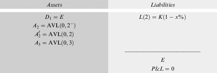
To have zero total cash flow and P&L for the first period, the bank needs to charge the cost to keep the liquidity buffer on the yield of the asset it buys from retail customers. It is clear this cost can be made small by reducing the preference for liquid securities and/or by reducing the survival period, although it is rather uncommon to set the latter shorter than one month. Anyway, if for the first period the yield requested on asset A3 is (r + sA + sB + LBC(1)/A3) (implying an expected return of (r + sB + LBC(1)/A3)), then we can restore an equilibrium condition with no cash imbalances or losses.
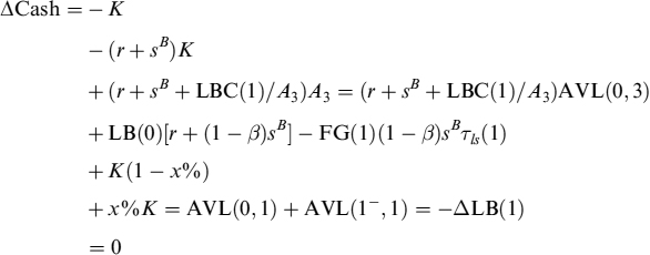
and the balance sheet is:
For subsequent periods, using an analysis identical to that just presented, the LB cost can be shown to be LBC(2) = βsBLB(1) + FG(2)(1 − β)sBτsv(2) and LBC(3) = 0. We can immediately see that the LBC for the last period is always nil, since the rollover of the debt stops and no LB needs to be kept. All the costs related to the buffer have to be charged on the yield of asset A3 at the appropriate times, in our case 1 and 2. We will see later on how to adjust the yield to include the liquidity buffer in a more standardized way.
7.3.3 Liquidity buffer costs when stressed scenarios do not occur
Proposition 7.3.7. In the presence of funding costs, when assumed stressed conditions do not occur, oversizing of the liquidity buffer does not produce unexpected costs if the bank either: (i) reinvests the unnecessary portion of the buffer in assets on which it can charge the actual costs of the buffer (which are different from those forecast at time T0 under stressed conditions), or (ii) shrinks the balance sheet simultaneously reducing the amount of issued debt and of the liquidity buffer, just as if stressed conditions actually manifested themselves.
As we did for the case of an economy where default risk does not exist, we now study what happens if the buffer has not been utilized because a stressed scenario either did not occur or manifested itself in a weaker form. Assume, for example, that at time T1 = 1 the rollover of the debt could be performed without any problem, so that the expected utilization of the LB for an amount K × (1 − x%) was not necessary. In this case there are three different rules the bank may follow:6
- The first rule is that the buffer is left unchanged if it is not utilized.
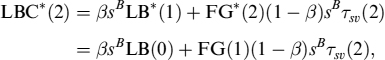
- At time T1 = 1: The debt can be rolled over for the entire amount, so that the new liability of the bank is K; the buffer is left unchanged, so we have LB*(1) = LB(0). The actual buffer at time 1, LB*(1), is different from the level of buffer LB(1) deduced by the amount needed to cover the funding gap of the stressed scenario. Total cash flow is still zero, although in this case there is no need to use the buffer; the P&L is zero as well, as can easily be checked. In the period [T1, T2], LB*(1) is invested in assets A2 and , which clearly will be held in an amount greater than forecast at time T0. The actual funding gap at time T2 will be equal to the forecast funding gap at time T1: FG*(2) = FG(1), which is also clearly different from the one predicted at time T0. The liquidity needed to buy an extra amount of these assets is provided by the expiry of asset . The return on the buffer will be:
R(2) = LB*(1)[r + (1 − β)sB] − FG*(2)(1 − β)sBτsv(2)
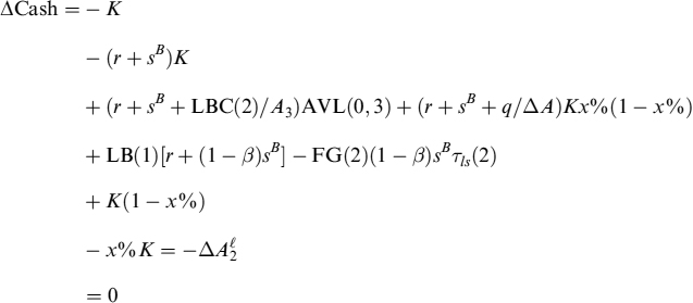
- At time T2 = 2 The LB and the rollover of the debt produces the same cash flows as those predicted at time T0 for the stress scenario at time T1 = 1. Stressed conditions regarding the rollover occur this time, so the buffer will be reduced accordingly (i.e., LB*(2) = (K(1 − x%) − AVL(0, 3))). If the bank charged the LBC(2) (computed on LB(2)) on the yield for the second period of the asset, we have total cash flow now as:
The funding gap is covered by a fraction of the maturing asset
in which the LB*(1) was invested, the remaining part is used to increase the amount of the investment in asset A3. Since there is no longer a need for a liquidity buffer, the amount left can be entirely used to buy an illiquid asset for an investment in the period [T2, T3]. Now,whereas
LBC(2) = βsBLB(1) + FG(2)(1 − β)sBτsv(2).
Since the expected levels of LB at the beginning of the activity at T0 = 0 implied that LB(0) > LB(1), which means that LB*(1) > LB(1) and FG*(2) > FG(2) we have that:
−LBC*(2) + LBC(2) < 0
so that total cash flow is negative. On the other hand, the balance sheet is:
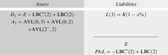
with P&L < 0, so that a loss is recorded.
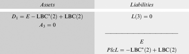
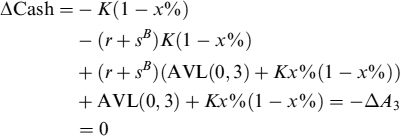
- At time T3 = 3: The debt is fully repaid with funds coming from the maturity of asset A3. Total cash flow is:
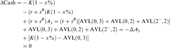
So we have zero cash flow and zero P&L. The only P&L arises from the second period and is negative as shown above. In fact, the balance sheet also shows a negative P&L:
To conclude, in the presence of funding costs for the bank, oversizing of the liquidity buffer for the periods it is needed causes a cost. This conclusion is different from when no funding spread is paid by the bank on its liabilities.
- At time T1 = 1: The debt can be rolled over for the entire amount, so that the new liability of the bank is K; the buffer is left unchanged, so we have LB*(1) = LB(0). The actual buffer at time 1, LB*(1), is different from the level of buffer LB(1) deduced by the amount needed to cover the funding gap of the stressed scenario. Total cash flow is still zero, although in this case there is no need to use the buffer; the P&L is zero as well, as can easily be checked. In the period [T1, T2], LB*(1) is invested in assets A2 and
- The second rule is that the buffer is abated to compensate for oversizing. The amount by which the buffer should be reduced has to be properly computed. Any excess buffer is used to increase the position in assets similar to A3. Without too great a loss of generality, we assume that the bank increases the amount of investment in A3.
- At time T1 = 1: The reduction of the LB can be shown to be equal to Kx%(1 − x%), so as to make the buffer adequate for a stressed scenario occurring at time T2 applied to an amount of debt that is not that predicted after a stressed scenario in T1, but the full amount K instead. The difference between the actual and predicted buffer is LB*(1) − LB(1) = x2%K: this higher amount has to be invested, according to the bank's liquidity preferences, in assets A2 and . The funding gap FG*(2) will also be higher than the predicted FG(2). Total cash flow is:
The line before the last one shows that the increase of the position in asset A3 generates a negative cash flow that is covered by a decrease of the LB. The remaining LB, higher than that predicted at time T0, increases available liquidity and is invested according to the bank's policy. The cost of the LB for the first period, LBC(1), is defined as above and is the one computed at time T0. The balance sheet is:
which shows zero P&L and a buffer LB*(1) = x%K that is different from LB(1), the level supposed if the stressed scenario at 1 happened.
- At time T2 = 2: Stressed conditions regarding the rollover occur this time, so the buffer will be reduced accordingly (i.e., LB*(2) = Kx% − Kx% = 0). At time T0 the bank charged LBC(2) = βsBLB(1) + FG(2)(1 − β)sBτsv(2) on the yield of the asset for the second period, but the actual cost for the buffer is LBC*(2)= βsBLB*(1) + FG*(2)(1 − β)sBτsv(2). Since it is easy to show that LB*(1) = x%K > LB(1) = x%(K(1 − x%) and hence FG*(2) > FG(2) (the actual buffer is greater than predicted), we have a negative total and the balance sheet would show a loss equal to q = LBC*(2) − LBC(2). If this additional cost, not forecast at time T0, is charged on the increase of the amount of asset A3, we have the following total cash flow
The balance sheet is:

so we still have zero total cash-flow and zero P&L.
Remark 7.3.1. The assumption that the bank is able to charge the extra cost originated by the oversized buffer on the yield of asset A3 should not be considered too restrictive. If A3 is an asset such as a mortgage or a loan, the bank has enough bargaining power to increase the contract rate of new deals so as to include the extra costs.
- At time T3 = 3: The debt is fully repaid with funds coming from the maturity of the asset A3 = AVL(0, 3) + Kx%(1 − x%) = K(1 − x%). Total cash flow is:
The balance sheet shows zero P&L as well:
So this rule does not produce negative or positive cash flows, as long as the excess buffer is used to buy new assets on which the bank is able to charge (besides the debtor's credit spread) its funding costs and the extra cost (q) due to the actual amount of the buffer larger than that predicted.
- At time T1 = 1: The reduction of the LB can be shown to be equal to Kx%(1 − x%), so as to make the buffer adequate for a stressed scenario occurring at time T2 applied to an amount of debt that is not that predicted after a stressed scenario in T1, but the full amount K instead. The difference between the actual and predicted buffer is LB*(1) − LB(1) = x2%K: this higher amount has to be invested, according to the bank's liquidity preferences, in assets A2 and
- The third rule is to reduce the amount of the buffer and at the same time reduce the amount of rolled-over debt just as if the stressed scenario actually occurred. The difference between this rule and the second one is that in this case the bank is actually reducing the balance sheet (both assets and liabilities) in much the same way as when a stressed scenario produces its effects, whereas in the second rule only the buffer was reduced, but the amount of debt was rolled over entirely since the market was regularly providing liquidity to the bank.
It is easy to check that, by following this rule, the bank has exactly the same total cash flow and P&L at the end of every period as if the stressed scenarios actually occurred. So the equilibrium conditions are preserved without any additional effort by the bank.
The analysis above, proving Proposition 7.3.7, provides the bank with guidance on the safest policy to implement in the management of the LB. In fact, depending on the bank's power to charge on the price of assets bought from retail customers the additional costs for the buffer as well, rule 2 or 3 can be followed so as to ensure that no P&L is generated when stressed conditions do not manifest themselves. On the other hand, rule 1 is clearly not able to prevent unexpected losses when the LB is oversized.
7.3.4 A more general formula for liquidity buffer costs
In a more general fashion, for a given liability used to fund the purchase of asset A, let the number of needed rollovers be nr with each rollover occurring on dates Trj, with j = 1, …, nr. Let τ(Trj) = Trj − Trj−1 be the period between two rollover dates, with the convention that τ(Tr0)= Tr1 − T0, with T0 equal to the reference date. Moreover, let τsv(Trj) be the survival period set by the bank before the rollover at time Trj, starting at time ![]() (usually
(usually ![]() month).
month).
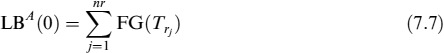
Total buffer is simply the sum of the funding gaps' nr rollover dates:
Let PD(0, T) be the discount factor from time 0 to time T.7 The total cost of the liquidity buffer for the purchase of asset A is the present value of the sum of the LBC for single periods:
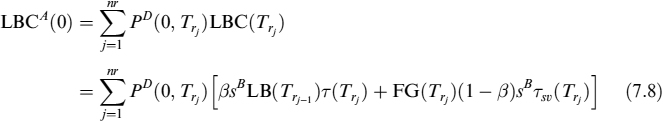
Total liquidity buffer costs depend on:
- The size of the FG at each rollover date: the size of the funding gap depends, in turn, on the stressed scenario assumed.
- The number of rollovers nr: they are determined once the maturity of the bought asset and of the liability used to fund it are determined.
- The bank's preference to invest all the LB in liquid assets traded actively in the market.
- The funding spread sB over the risk-free rate paid by the bank.
Remark 7.3.2. Although the analysis above and in the previous sections provides an in-depth insight into how to set up a liquidity buffer and how to compute and attribute related costs to the asset that generated its need, we should keep in mind that we are depicting a stylized economy. In a real-economy environment we have to account for additional sources of uncertainty that will alter, but not modify, the main results presented.
Looking at this in greater detail, the stochasticity of the interest rates and of the funding spread add an additional degree of riskiness that has to be properly measured and included in the calculation of the costs related to the LB.
Equation (7.8) can be made even more general by considering the fact that the bank might wish to split the fraction β of the liquidity buffer between liquid securities and cash. Let βs be the part of fraction β strictly allocated to liquid assets; furthermore let βc be the remaining part of β kept as cash. So β = βs + βc. The second term in (7.8) is modified to account for the fact that the bank loses the funding spread on the fraction of the LB it diverts to liquid securities, which is now βs; on the other hand, the bank also loses the risk-free interest rate on the fraction it keeps as cash that is absolutely unproductive of any yield. In conclusion, equation (7.8) reads:
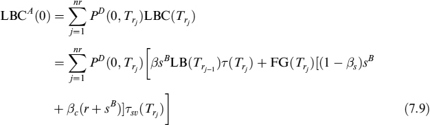
When period τ(Trj) is longer than one year, the spread sB cannot be used as indicated in formula (7.9). Typically, the spread will be applied to subperiods of one-year maximum length: let H be the number of these subperiods included in τ(Trj), so that τh(Trj) = T(h−1)rj − Thrj, for h = 0, …, H, T0rj= Trj−1 and THrj = Trj. Formula (7.9) modifies as:
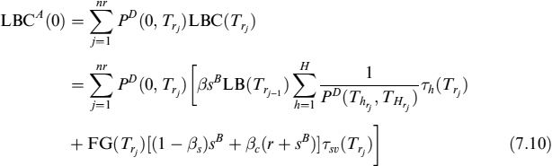
where we assumed that τsv(Trj) is always shorter or equal to one year in every case, so that sB simply compounded can be applied with no problems.
In the next example we will show how to put all the concepts and the formulae we have introduced so far into practice.
Example 7.3.1. Assume a bank has one liability in its balance sheet for an amount of 100; the liability has a typical duration of four years and bears a rollover risk of x% = 30% on expiry. The bank wants to invest in an asset expiring in 10 years; clearly there is a duration mismatch since two rollovers of the liability (at years 4 and 8) are needed to fund the purchase of the asset until its maturity. So the bank must first consider the available liquidity it can invest up to 10 years and as a consequence it will also determine the investments in illiquid and liquid assets expiring before the start of the two survival periods that include the rollover dates, and in liquid assets during the two survival periods.
The amount available for an illiquid asset expiring in 10 years is (recalling what we have shown above) 100 × (1 − 30%)2 = 49. Assuming the bank has a preference for liquid investment parameter β = 20%, the funds invested in illiquid and liquid assets up to the start of the two survival periods (i.e., up to 4− and 5−, adopting the notation used before) can easily be derived (see Table 7.1). For the maturity up to the start of the first survival period, 4−, the amount to be invested in illiquid assets is 24 and in liquid assets it is 6; the sum of 30 is the FG(4) = 100 × (1 − 30%). During the survival period [4−, 4] the full amount of 30 equal to the first funding gap is invested in liquid assets (as shown in Table 7.2).
Table 7.1. Term structure of liquidity to be invested in illiquid (AVLNL) and liquid (AVLL) assets for the investment in an asset expiring in 10 years with a liability that has a 4-year duration
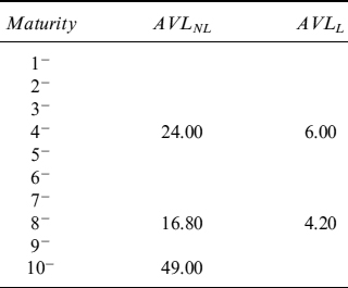
Table 7.2. Term structure of liquidity to be invested in liquid (AVLL) assets during survival periods, for the investment in an asset expiring in 10 years with a liability that has a 4-year duration
| Maturity | AVLL |
| 1−, 1 | |
| 2−, 2 | |
| 3−, 3 | |
| 4−, 4 | 30.00 |
| 5−, 5 | |
| 6−, 6 | |
| 7−, 7 | |
| 8−, 8 | 21.00 |
| 9−, 9 | |
| 10−, 10 |
Now, let us assume that the risk-free interest rate is constant and equal to r = 3% p.a. further that the bank funding spread is constant at sB = 2% p.a. To compute total LBC we use formula (7.10): the information we need on the amount of the liquidity buffer for each period and the amount of the funding gap on the rollover dates, is shown in Table 7.3. The discount factors are shown in Table 7.4.
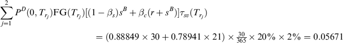
Assuming that βs = 20%, so that βc = 0%, and that the survival periods are both equal to one month, formula (7.10) yields:
LBCA(0) = 1.09256
This is the final result, which is the sum of:
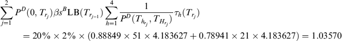
and
Table 7.3. Amount of the liquidity buffer and the funding gap for the investment in an asset expiring in 10 years with a liability that has a 4-year duration
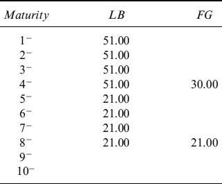
Table 7.4. Discount factors for maturities from one to 10 years, assuming a constant 3% annual risk-free rate
| Maturity | PD(0, T) |
| 1 | 0.97087 |
| 2 | 0.94260 |
| 3 | 0.91514 |
| 4 | 0.88849 |
| 5 | 0.86261 |
| 6 | 0.83748 |
| 7 | 0.81309 |
| 8 | 0.78941 |
| 9 | 0.76642 |
| 10 | 0.74409 |
If βs = 15%, so that βc = 5%, then the second part of the formula would be:
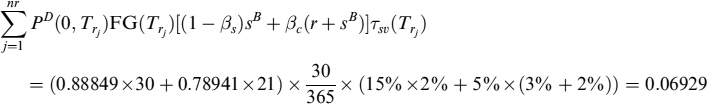
and total liquidity buffer cost would be:
LBCA(0) = 1.10499
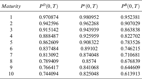
Table 7.5. Risk-free, spread and bank total discount factors for maturities from one to 10 years
Example 7.3.2. We assume that the asset expiring in 10 years in Example 7.3.1 is a loan to a counterparty: the capital is paid back at expiry whereas on a yearly basis the counter-party pays interest. To focus on the LBC, we assume the counterparty is default risk free.
Given the data we used in Example 7.3.1, the bank first derives the risk-free PD(0, T) and the funding spread Ps (0, T) discount factors, so that the total discount factors including the bank's funding spread are PB (0, T) = PD(0, T)Ps(0, T). These are easily found in our simplified example: let r* = ln(1 + r) and s* = −ln(1 + r + s) − r*; then PD(0, T)= e−r*T, Ps(0, T) = e−s*T and PB(0, T) = PD(0, T)Ps(0, T). The values are shown in Table 7.5.
To find the fair yearly rate c that the counterparty has to pay, the bank uses the following relation:
From Example 7.3.1 we know that A = 49 and LBCA(0) = 1.09256 (when βs = 20%). So we get:
![]()
If liquidity buffer costs were nil, the fair rate would be 5.00% (i.e., just the risk-free rate plus the funding spread), as it is easy to check by setting LBCA(0) = 0 in the formula above.
7.4 FUNDING ASSETS WITH SEVERAL LIABILITIES
Usual banking activity is run by funding the purchase of assets with a wide range of liabilities, different both in type and maturity. We generalize the results of the previous section by assuming that two liabilities (e.g., two bonds) with different maturities are issued. We also assume that there are two different funding gaps related to each of the two liabilities, depending on one being sold to retail customers and the other to professional investors.
Assume that the bank wants to finance an asset with maturity at T3 = 3 by two bonds L1 and L2, the first maturing at T1 = 1 and the other maturing at T2 = 2; both bonds are issued for amounts, respectively, equal to K1 and K2. Assume that the funding gap at time 1 for bond L1 is for x1% of the amount to roll over, whereas for bond L2 it is for x2%. The available liquidity at time 0 from bond L1 is:
AVL1(0, 3) = K1 × (1 − x1%)2
since two rollovers are needed at 1 and 2. From bond L2 the available liquidity is:
AVL2(0, 3) = K2 × (1 − x2%)
because only one rollover is necessary at 2. Total liquidity that can be invested is:
AVLT(0, 3) = AVL1(0, 3) + AVL2(0, 3)
and it is used by asset A with maturity T3 = 3, so that A = AVLT(0, 3). The LB at time 0 is:
LB(0) = K1 + K2 − AVLT(0, 3)
The LB can be seen as the sum of two separate liquidity buffers, each covering its reference bond's funding gap in a stressed scenario. Computing the cost of the LB is straightforward, once the TSFu has been defined along the lines adopted in Section 7.3.2 in the case of a single liability, since it is little more than the sum of the costs of the two buffers considered separately:
![]()
More generally, if the purchase of asset A is financed with N liabilities, of which M ≤ N has a maturity shorter than the asset, then total LB is:
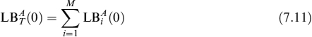
and the total cost of the liquidity buffer is:
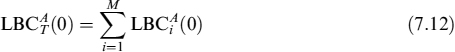
where ![]() and
and ![]() are, respectively, defined in equations (7.7) and (7.9) (or (7.10)).
are, respectively, defined in equations (7.7) and (7.9) (or (7.10)).
7.5 ACTUAL SCENARIOS SEVERER THAN PREDICTED
As already pointed out, stressed scenarios are designed to account for the severest liquidity conditions the bank may face at any given level of confidence (say, 99%). All scenarios producing even heavier difficulties but with a probability of occurrence below 1% (= 100 − 99%) are not considered, but in practice they are accepted as an intrinsic risk related to banking activity that cannot be ruled out.
The fact that unlikely scenarios can actually occur should in theory bankrupt the bank. Nevertheless, since liquidity stress does not imply immediate default, some strategies can be implemented although they cannot be defined within “equilibrium” liquidity policies and can be seen as an action of last resort to try and save the bank from default.
There are two strategies that can be identified for such severe scenarios.
- Immediately use all the available LB, even if allotted to future stressed scenarios, for the part invested in assets that are liquid and readily tradeable in the market.8 If this strategy is successful, the bank has to reintegrate the buffer for ensuing rollover dates.
- When no liquid assets are in the balance sheet and when the market still provides short-term liquidity to the bank, finance the greater-than-expected funding gap with short-term debt. This strategy can also be implemented after the one above has been activated but cannot be repeated given balance sheet constraints.
More specifically, let L1 be a liability expiring in T1 = 1 used to finance asset A3 maturing at T3 = 3. There are two rollover dates and a LB is built accordingly. On the first rollover date the funding gap FG*(1) exceeds the forecast stressed scenario and is even bigger than the entire LB available, so that FG*(1) > LB(0).
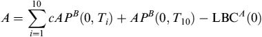
The bank may have invested the buffer in readily tradeable assets for the fraction β, so that this fraction can be used to cover any abnormal funding gap. Let us indicate by y%K = FG*(1) − FG(0) − βLB(1) the amount of the funding gap exceeding that assumed in the stressed scenario minus the fraction β invested in the marketable assets of the residual buffer still available at time 1. Assume also that the bank can issue a short-term liability L2 maturing at T3 = 3. Moreover, this liability needs to be rolled over twice, since its duration is single period, and the stressed scenario predicts a funding gap of z% for each rollover date.
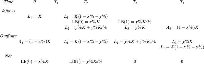
In the table below we show variations of the liabilities and of the assets, including the liquidity buffer. At time T2 the liquidity buffer built at time T0 is not enough to cover an abnormal stressed scenario, so that short-term funding is used to cover the funding gap by issuing new debt L2. Furthermore, this debt has to be rolled over at T3, so a liquidity buffer LB(1) is formed based on the assumption that z% in a stressed scenario cannot be financed. Actually. we suppose that this stressed scenario happens at T3, so that the buffer is used to cover the funding gap. Finally, at T4 the short-term debt L2 is paid back with proceeds from asset A4.
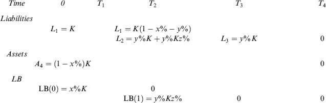
In the table below we show the cash flows at each time associated with variations of the liabilities, of the assets and of the liquidity buffer.
The problem with the second approach the bank can follow in an abnormal stressed scenario is that it clearly suffers from the fact that short-term financing covering funding gaps also may not be fully protected by the liquidity buffer, since other abnormal scenarios may happen. So this approach should be seen as an extreme measure to avoid bankruptcy when scenarios manifest themselves with a severity beyond the chosen confidence level (e.g., 99%), but they should not be used as sound practices to establish funding and liquidity buffer policies.
7.6 THE TERM STRUCTURE OF AVAILABLE FUNDING AND THE LIQUIDITY BUFFER
Having analysed how the liquidity buffer is generated by the maturity mismatch, how its amount is determined and what are the associated costs, we will now focus on how it is possible to build a generic term structure of available funding, considering both the liquidity that can be invested in illiquid and liquid assets. We also assume a situation somewhat nearer to reality than the stylized one sketched in the previous sections.
More specifically, we suppose that the bank funds its activities by means of a fairly wide range of funding sources, each one characterized by its own typical duration and funding spread. All funding sources contribute to the financing of activities indistinctly and proportionally to the weight of each of them. If we accept this assumption, keeping in mind predicted funding gaps, then the TSFu is readily derived.
Let the number of funding sources be M and let T1m be the expiry of each funding source for m = 1, …, M. We assume that each source has a typical duration that is the same in the future as well, when the liability will be rolled over by the bank; this means that the typical duration for each source is τm. Assume we want to build the TSFu between time T0 and time Tb (i.e., TSFu(T0, Tb)). For simplicity's sake, we assume that each funding source starts at time T0, meaning that all corresponding liabilities are sold at time T0; we also assume that the typical duration of each funding source is contained an integer number of times in the period [T0, Tb] (e.g., 3 times, but not 3.7 times): this assumption is easily relaxed and the approach we are sketching here can be extended to more general cases when some or all liabilities do not start at T0.
Under the assumptions above, the number of rollovers for the m-th funding source is:
![]()
We can determine the TSFu for this funding source at the end of the horizon we are considering, which is Tb, given that the initial amount of the corresponding liability at time T0 is Lm = L(T0, T1m), where T1m is the expiry of the m-th funding source, corresponding to the first rollover date. The available liquidity is computed in the same way as done in Section 7.3: indicating by xm% the percentage of the amount that the bank is not able to roll over on each of Nm rollover dates. In this way, we get the available liquidity for investments in illiquid assets up to time Tb:
AVLNL(T0, Tb) = Lm(1 − xm%)Nm
which is the initial amount of funds Lm raised at time T0 by source m, including the deduction of xm% on each rollover date for Nm number of times. The difference between this quantity and the initial amount Lm contributes to the liquidity buffer.9
We also know, from the analysis above, that the liquidity buffer can be reinvested in liquid and illiquid assets, according to proportions indicated by the bank's preference parameter β to invest in liquid securities. Let us examine how the LB is invested for the m-th funding source: first consider ![]() , the quantity of LB that can be invested in non-liquid assets (such as loans), up to the time
, the quantity of LB that can be invested in non-liquid assets (such as loans), up to the time ![]() when the survival period including the first rollover starts: this is basically an amount equal to the funding gap for the first rollover, taking into account the parameter for the preference of liquid assets β, so (1 − β) is invested in illiquid assets:
when the survival period including the first rollover starts: this is basically an amount equal to the funding gap for the first rollover, taking into account the parameter for the preference of liquid assets β, so (1 − β) is invested in illiquid assets: ![]() .
.
The formula can be generalized in a straightforward way to the Nm rollovers of the m-th funding source, so as to obtain the available liquidity for investments in illiquid assets from time T0 to the beginning of the survival periods for the Nm rollover date, ![]() , for nm = 1,…, Nm:
, for nm = 1,…, Nm:
![]()
For the same periods, a complementary fraction β is invested in liquid assets, so that the corresponding available liquidity is:
![]()
Finally, during the survival periods τnm, referring to the n-th rollover of the m-th funding source, the available liquidity must be invested in liquid assets for an amount equal to the predicted funding gap FGm(Tnm), so that we have (recalling that ![]() :
:
![]()
Collecting all results and summing over M funding sources, we have that the TSFu is:
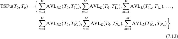
In Example 7.6.1 we show how to build the TSFu in practice.
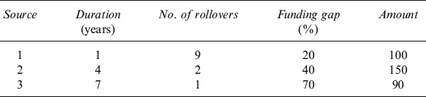
Example 7.6.1. In this example we show how to build a complete TSFu for a given time horizon. Assume we have three funding sources (M = 3) and that the horizon is between times Ta = 0 and Tb = 10. The three sources have the typical durations shown in Table 7.6, where the number Nm of rollovers, the funding gap percentage xm% (for m = 1, 2, 4) and the initial amount in 0 are also indicated.
Table 7.6. Input data for the three funding sources.
We assume that the preference parameter to invest in liquid assets is β = 20%.
For the first liability, the number of rollovers is 9, so that the available liquidity after the last rollover, until the end of the chosen horizon of 10 years, is AVLNL(0, 10) = 100(1 − 20%)9 = 13.42. Similarly we have that AVLNL(0, 10) = 150(1 − 40%)2 = 54 and AVLNL(0, 10) = 90(1 − 70%)2 = 27.
The liquidity buffer for each source can be reinvested in illiquid assets for a fraction 1 − β = 80% until the first rollover date. So, for example, for the first source and the first rollover date at time 1, we have AVLNL(0, 1−) = (1 − β)FG1(1) = 80% × 20% × 100 = 16, for the second source the available liquidity given by the LB to be invested in non-liquid assets is AVLNL(0, 4−) = (1 − β)FG2(4) = 80% × 40% × 150 = 48 and for the third source AVLNL(0, 7−) = (1 − β)FG3(7) = 80% × 70% × 90 = 50.40.
The amount that has to be invested in liquid assets from the LB generated by the funding source 1 is AVLL(0, 1−)= βFG1(1) = 20% × 20% × 100 = 4, for the LB generated by funding source 2 we have AVLNL(0, 4−) = βFG2(4) = 20% × 40% × 150 = 12 and for funding source 3 we have AVLNL(0, 7−) = βFG3(7) = 20% × 70% × 90 = 12.60.
Finally, during the survival period relating to each rollover date, an amount equal to the funding gap for that date has to be invested in liquid assets. For example, for the first rollover date of the first funding source AVLL(1−, 1) = FG1(1) = 20% × 100 = 20, for the second funding source AVLL(4−, 4) = FG2(4) = 40% × 150 = 60 and for the third funding source AVLNL(7−, 7) = FG3(7) = 70% × 90 = 63.
Table 7.7. Available liquidity that can be invested in illiquid assets for maturities up to 10 years generated by the three funding sources
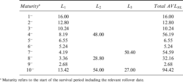
Table 7.8. Available liquidity that can be invested in liquid assets for maturities up to 10 years generated by the three funding sources
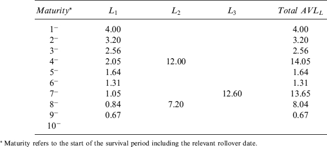
Performing computations for each funding source and for each rollover date, we come up with a complete term structure of available funding TSFu. The term structure of AVLNL for investments in illiquid assets generated by each funding source, and the total amount, is shown in Table 7.7. Analogously, Table 7.8 presents the term structure for investments in liquid assets. The amount to be invested in maturities included in the survival periods relating to rollover dates is shown in Table 7.9.
It is interesting to see how assumptions about the funding gap on rollover dates strongly affect the entire TSFu and hence the liquidity available for investments in illiquid assets (i.e., typical banking contracts with retails customers or companies) and in liquid assets (i.e., in securities actively traded in the market). Extreme cases of a funding gap equal to the amount to be rolled over (x% = 100%) prevent any form of maturity transformation if the bank wants to implement a robust and balanced investment and funding policy starting from the observation time. We will dwell more on the unintended (or even intended, we might think) consequences of the proposed international regulation on liquidity standards (see [101]).
Table 7.9. Available liquidity that has to be invested in liquid assets for maturities included in survival periods up to 10 years
7.6.1 The term structure of forward cumulated funding and how to use it
For practical purposes it is useful to build a term structure of forward cumulated funding (TSFCFu). This term structure shows the total funding available at each date, keeping in mind that it is always possible to safely use liquidity allocated to future expiries for shorter maturities.
The TSFu has been built based on the idea that the bank invests in illiquid assets according to investment in the longest possible maturity and to allocation of the resulting liquidity buffer. But this is not the only possible use of total available funding and we need a tool to effectively manage it: the TSFCFu serves this purpose.
For a given expiry, the bank can decide to use available funding for an illiquid asset as indicated by the TSFu, but it can also use all the funding allocated for longer expiries. For example, we know that the available funding for an asset expiring at time T = 3, funded with a liability expiring at T = 1 and of typical duration of one period, is K(1 − x%)3. Nevertheless, it is always possible to safely use the entire funding K for an investment in an illiquid asset expiring at T = 1, with no need to build any liquidity buffer since no rollover of the liability is needed.
When shorter expiry investments use the funding allocated for longer expiry investment, the need for a liquidity buffer decreases as a function of the number of rollovers no longer needed. Consequently, the need to allocate a fraction of the buffer to liquid assets should also correspondingly disappear. In practice, we can make two assumptions about investment in liquid assets:
- The bank still invests in liquid assets according to the TSFu produced using the methodology outlined above, assuming that investment in the illiquid asset with maturity Tb is the driving factor.
- The bank considers the investment in liquid assets for each maturity as a consequence of the need to build a LB, so that it is not necessary when investment in illiquid assets implies a smaller number of (or even no) rollovers.
If the bank adopts the first assumption, then forward cumulated available liquidity (FCAVLNL) from expiry Ti to the end of period Tb for the m-th funding source is computed as follows:
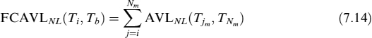
Equation (7.14) indicates that for each expiry Ti the forward cumulated available liquidity for illiquid assets is equal to the sum of available liquidity for illiquid assets for each expiry date from Ti to the end of the considered horizon Tb.
When the bank decides to adopt the second assumption, then the FCAVLNL also includes the fraction devoted to investment in liquid assets for each expiry. So we have:

The TSFCFu is then defined, for all M funding sources, as the following collection of FCAVL:
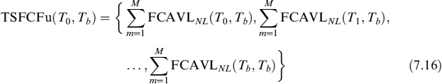
Although both assumptions can have an economic and financial rationale backing them, we tend to favour the second option since the first is too conservative and not really justified by any real liquidity risk. We will present an example in which the bank chooses the second assumption.
Remark 7.6.1. Although the two rules to build the TSFCFu have been presented as exclusively alternative, it should be noted that it is always possible to adopt a blended version of the two, by assuming that investment is the driver in the illiquid asset at expiry Tb, but that at the same time a fraction 1 − β of the AVLL increments of the forward cumulated available liquidity FCAVLNL. With respect to the second rule, there is a partial, instead of a total, contribution of liquidity devoted to liquid investments to the increase of available liquidity for illiquid investment.
Once the bank has built the TSFCFu, it can easily check what is the maximum available funding for investments in illiquid assets, considering the possibility to use sums allocated to future expiries. Use of the TSFCFu is subject to the following rules:
- when a bank utilizes funds allocated to a given expiry, the corresponding amount is deducted from the funds referring to all the other expiry dates of the term structure;
- there is a floor at zero, so that any entry of the TSFCFu can never go negative;
- the updated term structure can be used for other investments if funding is still available.
Both the TSFu and the TSFCFu are necessary to manage available funding. The TSFCFu allows the bank to understand how much is globally available on any expiry, given the current amount of funding at time 0, considering investments in illiquid assets with a duration smaller than the longest expiry in the term structure. Once the investment is decided by means of the TSFCFu, the TSFu indicates how to allocate the remaining funds for shorter expiries, so as to guarantee the building of a LB. Example 7.6.2 will clarify this idea with a practical application.
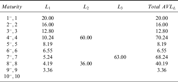
Example 7.6.2. We recall Example 7.6.1 and use all the data shown therein. We want to build the TSFCFu, given the TSFu shown in Tables 7.7–7.9. We work under the assumption that investments in illiquid assets for shorter dates require smaller amounts from the LB and hence smaller investments in liquid assets.
In Table 7.10 we show the FCAVLNL, broken down into its two components, and the TSFCFu, all of which include the three funding sources. The first entry in the column TSFCFUNL is the cumulated amount of column “Total AVLNL” of Table 7.7 (i.e., 290.88), whereas the first entry of the second column shows the same for the column “Total AVLL” of Table 7.8 (i.e., 49.12). The entry in the third column is the sum of entries of the first two columns. The rest of the table is built in exactly the same way.
In Figure 7.1 we compare that part of the TSFu that relates to illiquid investments using the TSFCFu: clearly, the two term structures converge at the same number at the end of the considered horizon Tb.
Assume the bank wants to invest the full amount available of 340 on expiry at time 1: this means that the bank uses all funds for an investment in illiquid assets maturing in 1 year. The available amounts for the following expiries are abated by the same amount, not going below zero for any expiry under any circumstances. In this case it is easy to check that available forward cumulated funding reduces to zero on every expiry. That would not be the case if the bank decided to invest a lower amount (say, 100), in an asset expiring at time 1, or an amount (say, 150) on expiry at time 5. In both these cases there would still be something left to invest for other expiries (as shown in Table 7.11).
Table 7.10. Term structure of forward cumulated funding and its components
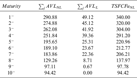
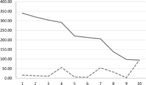
Figure 7.1. The TSFu for illiquid assets (dotted line) and the TSFCFu (continuous line). The x-axis shows the expiries whereas the y-axis the amount
Table 7.11. Term structure of forward cumulated funding after the bank decides to invest 340 or 100 in an asset expiring at time 1 (first and second column), or 150 in an asset expiring at time 5 (third column)
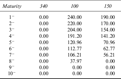
Joint use of the TSFu and the TSFCFu can be illustrated by the third case of Table 7.11, when the bank decides to use 150 for an asset expiring at time 5, out of a total available of 220.96 (as can be read from Table 7.10): the used funds represent ![]() of the total. This means that the bank needs to build a LB as indicated by the TSFu in Tables 7.7 and 7.8 (column “Total”) for the corresponding percentage. In Table 7.12 we show the investment in illiquid and liquid assets necessary to preserve a LB for the investment of 150 expiring at time 5. The amount invested in liquid assets in the survival periods before expiry 5 is shown in Table 7.13.
of the total. This means that the bank needs to build a LB as indicated by the TSFu in Tables 7.7 and 7.8 (column “Total”) for the corresponding percentage. In Table 7.12 we show the investment in illiquid and liquid assets necessary to preserve a LB for the investment of 150 expiring at time 5. The amount invested in liquid assets in the survival periods before expiry 5 is shown in Table 7.13.
Table 7.12. Liquidity allocated to illiquid and illiquid assets maturing before time 5 to build the liquidity buffer needed for an investment of 150 expiring at time 5
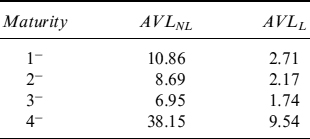
Table 7.13. Investment in liquid assets in the survival periods before time 5 for the liquidity buffer needed for an investment of 150 expiring at time 5
| Maturity | AVLL |
| 1−, 1 | 13.58 |
| 2−, 2 | 10.86 |
| 3−, 3 | 8.69 |
| 4−, 4 | 47.68 |
7.7 NON-MATURING LIABILITIES
Among banks' main funding sources are non-maturing liabilities, typically sight deposits. In fact, although their duration is in theory nil because they can be closed (totally or partially) on demand by creditors,10 in practice their actual duration is longer. In some cases, depending on the “stickiness” of the deposits, the duration can be around 5/7 years or longer.
Non-maturing liabilities can be seen as any other fixed maturity liability, except that the duration is stochastic and their rollover does not occur on predefined dates known at the observation time. In practice, the amount of non-maturing liabilities is assumed to follow some decaying pattern over time such that the bank can pretend they are rolled over on a periodic basis with a runoff factor, analogously to other liabilities we have analysed above. We investigate here how non-maturing liabilities are involved in the building of the TSFu and the size of the liquidity buffer needed to cover funding gaps brought about by their rollover.
Let NML(T0) be the amount at time T0 of non-maturing liabilities the bank has in the balance sheet. Let Tb be the end of the period the bank considers necessary to determine the TSFu, and let the entire period [T0, Tb] be divided into NNML subperiods. The bank can assume that a fraction of xNML% of the total amount is lost during each subperiod,11 so that it can actually assimilate the end of each subperiod to a rollover date, and the subperiod itself to a survival period of length equal to τsv(TnNML) = TnNML − T(n−1)NML, for n = 1, …, NNML.
Under these assumptions, it is quite easy to apply the concepts introduced above for maturing liabilities to non-maturing liabilities. More specifically, the available liquidity for investments at the end of the considered horizon Tb is:
The difference between this available liquidity and the initial amount NML(T0) is the liquidity buffer needed to cover funding gaps relating to the (fictitious) rollovers of non-maturing liabilities.
Since each survival period τsv(TnNML) clashes with the entire period between two (fictitious) rollover dates, there is no investment available in non-liquid assets for that part of the liquidity buffer needed to cover each funding gap
FG(TnNML) = xNML%NML(T0)(1 − xNML%)nNML,
so that the entire amount is fully held in liquid assets:
AVLL(T(n−1)NML, TnNML) = FG(TnNML)
On the other hand, what has to be invested in fully liquid assets during a given survival period τsv(TnNML ) can be invested in less liquid assets expiring just before its start. In this case we have:
AVLNL(T0, T(n−1)NML) = (1 −β)FG(TnNML)
where we have also included the preference of the bank for investment in liquid assets via the parameter β. The complementary part can also be invested in liquid assets so that the total amount of investment in them for each period is:
AVLL(T0, T(n−1)NML) = βFG(TnNML)
Thus the term structures of funding and forward cumulated funding for the source of non-maturing liabilities can easily be derived in much the same way as above.
Example 7.7.1. The bank wants to compute the TSFu and the TSFCFu for a period of 2 years. The entire period is divided into NNML = 24 subperiods of length one month each. In each subperiod the bank supposes that xNML % = 5% of the outstanding amount is lost by depositor runoff. The one-month periods are also equal to the survival periods for each (fictitious) rollover. Assume that the bank has an amount of non-maturing liabilities equal to NML(T0) = 100 and that its preference parameter for liquid investments is β = 20%.
It is straightforward to compute the available liquidity for non-liquid assets up to the 24th month:
AVLNL(0, 24M) = 100(1 − 5%)24 = 29.20
During each survival period, a quantity equal to the corresponding funding gap is invested in liquid assets. For the first period, which is a month in our example, we get:
AVLL(0, 1M) = 100 × 5% = 5
For the second survival period, the amount of NML after runoff is 100 − 5% × 100 = 95. The liquid investments for this period will be:
AVLL(1M, 2M) = 95 × 5% = 4.75
Table 7.14. Term structure of available liquidity that can be invested in illiquid and liquid assets up to the end of each period of one month
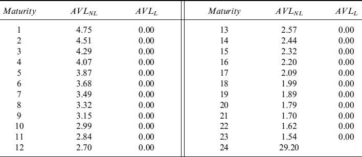
Up to expiry of the first survival period the bank can invest in illiquid assets an amount equal to the amount it needs for the subsequent survival period, keeping its preference for liquid assets in mind. For the first period we have:
AVLNL(0, 1M) = 4.75 × (1 − 20%) = 3.80
For the same period the complementary fraction 20% is invested in liquid securities:
AVLL(0, 1M) = 4.75 × 20% = 0.95
So that for the first period total AVLL (0, 1M) = 5.00 + 0.95 = 5.95.
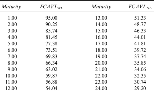
The entire TSFu is shown in Tables 7.14 and 7.15. In Table 7.16 we show the TSFCFu.
Table 7.15. Term structure of available liquidity that can be invested in liquid assets in each survival period of one month
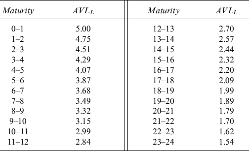
Table 7.16. Term structure of forward cumulated funding for non-maturing liabilities
7.7.1 Pricing of NML and cost of the liquidity buffer
Proposition 7.7.1. The liquidity buffer cost incurred by the purchase of assets funded by NML is equal to zero if the bank can pay interest equal to a fraction of the risk-free interest rate that is applied for the repricing period. This fraction depends on the expected daily withdrawal rate on the outstanding NML. If the bank for some reason has to pay an interest rate greater than a fraction of the risk-free rate, then the liquidity buffer cost is greater than zero.
Non-maturing liabilities can be typically withdrawn on demand by creditors (customers) as, for example, in the case of sight deposits. As such banks need to keep a liquidity buffer that is not only invested in liquid assets, at least a fraction of the buffer needs to be kept in cash so as to cover outflows that can be brought about by withdrawals on any day.
In practice, the bank estimates a daily withdrawal rate from the runoff rate xNML%. The simplest way to do this is to consider the number of days in a survival period and use the following relation:
![]()
where ![]() is the daily withdrawal rate and nd(n) the number of days in the n-th survival period; the daily withdrawal rate will then be:
is the daily withdrawal rate and nd(n) the number of days in the n-th survival period; the daily withdrawal rate will then be:
![]()
This basic method can be made much more sophisticated by analysing specific calendar dates and expected withdrawals for each of them, but this is beyond the scope of the current analysis. The assumption the bank is making in this simple case is that any drop in the ![]() occurs daily at a constant rate consistent with the runoff rate over the entire survival period.
occurs daily at a constant rate consistent with the runoff rate over the entire survival period.
If ed(n) have elapsed from the start of the n-th survival period and NML(TnNML) is the amount of NML at the beginning of the period, then the expected amount left is equal to:
![]()
where Ted(n) is the date corresponding to ed(n) after the start of the n-th survival period.
This information is useful to the bank when deciding the rate it is willing to pay on NML. It should be stressed that, since creditors providing funds via NML are typically retail customers, the bank benefits from having strong bargaining power in setting the rate to pay; on the other hand, competitive forces operating in the banking industry should not be completely overlooked, because they still play a role in setting the general level of the rate paid on such funding sources.
It is also worthy of mention that the rate is variable and repriced periodically to update it and put it in line with market interest rates. Usually, the repricing period is linked to a short-term rate such as the 3-month Libor/Euribor or Eonia rate.
When a bank has the bargaining power to set the rate paid freely, the fair level should consider the repricing period, the runoff rate xNML% and the daily withdrawal rate ![]() . Assuming the repricing period clashes with the survival period (say, one month), then the bank can use the following relationship to compute the fair level to pay on NML between the start and the end of the period:
. Assuming the repricing period clashes with the survival period (say, one month), then the bank can use the following relationship to compute the fair level to pay on NML between the start and the end of the period:

where NML(TnNML) is the amount of NML at the beginning of the period. Equation (7.18) states that the interest d that the bank pays on the amount of NML each day during the survival period (left-hand side), is equal to investment in liquid assets (whose expected return is the risk-free rate, as shown above) for an amount that is equal to NML available minus expected daily withdrawals (right-hand side).
Looking at this in greater detail, on every day the bank has an expected amount equal to ![]() in its liabilities on which it pays the rate d; on the other hand, the bank can invest only
in its liabilities on which it pays the rate d; on the other hand, the bank can invest only ![]() in risk-free liquid assets, since an amount equal to expected daily withdrawals,
in risk-free liquid assets, since an amount equal to expected daily withdrawals, ![]() , has to be kept as cash that earns 0. It is straightforward to compute the fair level that the bank should be willing to set on NML at the start of the repricing period:
, has to be kept as cash that earns 0. It is straightforward to compute the fair level that the bank should be willing to set on NML at the start of the repricing period:
where ![]() , which is obviously smaller than 1. Equation (7.19) states that the fair rate on NML, which is refundable on demand, is the risk-free rate minus the amount of cash needed to cope with expected daily withdrawals. Consequently, the funding spread sB that the bank pays is now computed over the fair risk-free return αr, and not simply r; so for NML the funding spread is sB = max[d − αr;0]. If the bank has reasonable bargaining power, then d − αr ≤ 0, which means the bank pays no funding spread for this source of funding. Sometimes the bank either has very weak bargaining power or competition in the banking industry is so fierce as to push NML rates above the fair level αr, such that a positive funding spread may result.
, which is obviously smaller than 1. Equation (7.19) states that the fair rate on NML, which is refundable on demand, is the risk-free rate minus the amount of cash needed to cope with expected daily withdrawals. Consequently, the funding spread sB that the bank pays is now computed over the fair risk-free return αr, and not simply r; so for NML the funding spread is sB = max[d − αr;0]. If the bank has reasonable bargaining power, then d − αr ≤ 0, which means the bank pays no funding spread for this source of funding. Sometimes the bank either has very weak bargaining power or competition in the banking industry is so fierce as to push NML rates above the fair level αr, such that a positive funding spread may result.
Assume the bank wants to finance the purchase of asset A expiring at Tb with NML and the number of related (fictitious) rollovers is NNML; each rollover occurs on dates Trj, with j = 1, …, NNML. The available amount AVLNL (T0, Tb) that can be funded is given by equation (7.17).
To compute the LB, we can resort to equation (7.9) and adapt it to the specific case of NML. First, we note that since the survival period clashes with the entire period between two rollover dates, a fraction of the liquidity buffer equal to the funding gap for the relevant period is completely invested in liquid assets and/or in cash. Second, we need to keep in mind that this amount of the FG for each survival period varies with time. In fact, at date Ted(n) between the start and the end of a survival period, corresponding to ed(n) days after the start of the n-th survival period, an amount needed to cover withdrawals on outstanding NMLTnNML is held in cash:
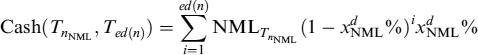
which is the expected amount at time Ted(n) (considering a daily withdrawal rate of ![]() ), multiplied by the withdrawal rate of
), multiplied by the withdrawal rate of ![]() . The amount of the buffer invested in liquid assets is:
. The amount of the buffer invested in liquid assets is:
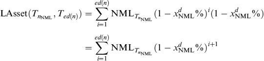
For the generic survival period τ(Trj) = τsv(Trj) = Trj − Trj−1 the cost of the buffer is:
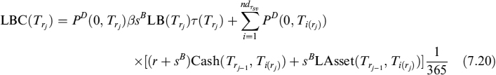
where Ti(rj) is the date corresponding to i days after the start of the period Trj−1. It should be stressed that the LB does not include the fraction relating to the survival period, (so it is LB(Trj), instead of LB(Trj−1) as in equation (7.9)). The total cost of the liquidity buffer is as usual the sum of the LBC for all the survival periods until the maturity of asset A:
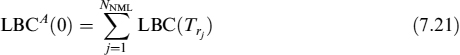
We can now examine the two cases of nil funding spread or positive funding spread on NML, and their effects on the cost of the liquidity buffer:
- The bank has enough bargaining power to set d = αr, or at an even lower level. In this case the funding spread sB is zero, so that from (7.20) one immediately sees that the LBC to charge on asset A funded with NML is just the amount of cash kept in the buffer times the risk-free rate.
- The bank has to pay some rate d > αr on its NML so that the LBC is not nil and its value is computed by means of equation (7.21).
Table 7.17. Amount invested in liquid assets and cash on each day of investment in an asset funded by non-maturing liabilities
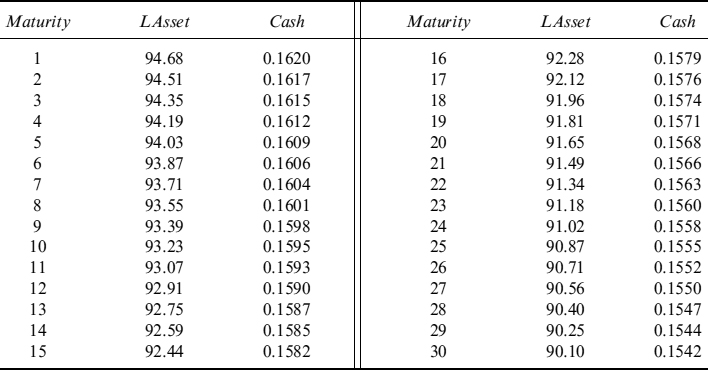
Example 7.7.2. Assume we are at the same outset as in Example 7.7.1 and that we want to compute the LBC related to the purchase of an asset expiring in one month, fully funded with the NML outstanding at time 0, which we recall is 100. Available funding can be obtained from the TSFCFu shown in Table 7.16: it is 95, which implies a LB(Tr0) = LB(0) = 5. The daily withdrawal rate is ![]()
![]() .
.
Let us assume a constant risk-free interest rate equal to r = 3% p.a. for any maturity: the fair NML rate should be d = 3% ×(1 − 0.17%) = (1 − 0.17%) = 2.995%. We suppose the bank is unable to set this rate on NML at this level, but has to pay a higher rate so that d − αr = 2%. So the funding spread sB = 2%.
The liquidity buffer cost relating to this investment can easily be computed by considering the fact that we have just 1 period, so NNML = 1; the period between the start and the first rollover is τ(Tr1) = 30/365 = 0.0822. In Table 7.17 we show the amount of LAsset and Cash that the bank holds on each day between the start and end of the investment. It is straightforward to calculate the single components of formula (7.20) and then of formula (7.21) (in this example we just have a single term to consider in the latter). Noting that LB(Tr1) = LB(1) = 0 in this case, we just need to compute the two summations in the second part of (7.20) (i.e., ![]() and
and ![]() .). The results are shown in Table 7.18, and we get LBCA(0) = 0.1525.
.). The results are shown in Table 7.18, and we get LBCA(0) = 0.1525.
Table 7.18. Calculations of the LBC for investment in an asset funded by non-maturing liabilities
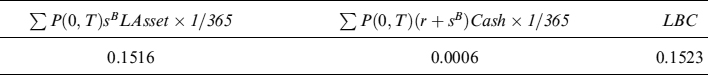
7.8 THE SECOND CAUSE OF THE LIQUIDITY BUFFER: COLLATERAL MARGINING
In current financial markets, collateralization of derivative contracts, at least of those dealt between institutional investors, is the normal rule since it is considered the best way to mitigate or almost remove the counterparty credit risk. On the other hand, liquidity risk increases because there is a higher probability that cash or eligible (liquid) assets (typically bonds) are needed to post a collateral margin when the NPV of the contracts with a counterparty becomes increasingly negative. Moreover, one should not disregard the possibility of receiving cash or eligible assets when the NPV is positive: a positive windfall in liquidity risk management.
Derivatives contracts are subject to collateralization according to:
- CSA agreements: Thes are bilateral agreements between two institutional agents (generally banks) to periodically exchange collateral to cover the change in NPV of a derivative contract or a portfolio of contracts. It is almost standard practice today to have a daily exchange of collateral.
- Multilateral margining via central counterparties: Multilateral netting and margining of derivatives contracts is operated via clearing houses. In this case collateral is also exchanged once or more times a day.
The need for cash or eligible assets arises mainly when contracts cannot be replicated by a suitable strategy involving primary assets, as is the case for interest rate swaps and FRAs (see Chapter 12): hedging for those contracts is attained by reversing the same contract with another counterparty. If both trades (the original and the second traded for hedging purposes) are margined in the same way (say, daily) then there is no liquidity risk since the cash (or assets) needed to post collateral for one on them is precisely compensated by the collateral received on the other. When the two contracts are not collateralized in the same way, then the asymmetric behaviour of cash flows paid and received brings about liquidity risk. This situation usually occurs in banking activity when the bank trades with corporate clients (with whom there are agreements to post collateral on an infrequent basis or none at all) and hedges with other banks (with whom CSA agreements are typically signed on a daily basis).
7.8.1 A method to set the liquidity buffer for derivative collateral
Proposition 7.8.1. The liquidity buffer to cover collateral margin calls is equal to the minimum negative value of the contract during its life. The minimum can be computed at an expected level, by expected negative exposure, or at a level with a given confidence level, by potential future exposure.
We sketch a method to set the level of the LB when collateral agreements (such as a CSA) or multilateral margining via a clearing house is operating. We assume for simplicity's sake that collateral is posted daily, either in cash or eligible bonds, according to variations in the contract's NPV. The method consists of the following steps:
- Determine the expected negative exposure (ENE) or the potential future exposure (PFE) of the contract until expiry. ENE is defined as expected negative NPV, computed at time T0, of the value V of a contract at time Ti, given that it expires at Tb,
Expectation in this case is taken according to the risk-neutral measure, indicated by the superscript Q of the expectation operator, which takes forward levels quoted in the market as expected values and levels implied from quoted option prices as volatilities. Expectation can also be taken according to a real-world measure P, in which case we use means and variances estimated statistically from actual price movements.
The PFE is defined similarly as the minimum Vα reached by the value V at time Ti, such that the probability that the value is lower than (1 − α):
such that
- Let period [T0, Tb] be divided into N subperiods. The LB that the bank needs to build is given by fraction γ, which depends on the risk aversion of the bank and on the minimum ENE of PFE for each of the subperiods:
or
where Δ− = min[ENE(T0, Ti) − ENE(T0, Ti−1);0] is negative variation in ENE between the start and end of each subperiod (similar notation applies to the PFE). We implicitly assume here that ENE or PFE are constant during each subperiod [Ti−1, Ti]. Equations (7.25) and (7.26) state that the liquidity buffer is the minimum negative (expected or at a given confidence level) value of the contract.
The idea is that the bank wants to make sure that it is able to meet the requests for collateral by the counterparty. The collateral that will be posted during each period is given by ENE as the expected level, or by PFE at the maximum level with a given confidence level. The bank can adopt either measures, being more conservative with PFE and with a higher value of γ that could be set up to 100%.
- The survival periods during the life of the contract are not determined according to (possibly fictitious) rollover dates, but they are simply contiguous subperiods, of a given length (say, one month), during which the liquidity buffer must be invested for an appropriate amount in liquid assets to meet collateral posting requirements. So, the N subperiods, for which we computed ENE or PFE, also clash with the survival periods included in the period [T0, Tb]. In each survival period τsv(Ti) the LB is invested in liquid assets for an amount equal to variation in ENE, since they can be converted into cash or even used as collateral themselves.12 The remaining buffer can be invested in illiquid assets and liquid assets, according to parameter β, by suitably choosing their expiries such that at the start of each survival period an amount equal to γ times the variation in ENE or PFE is available for investment in liquid assets.
7.8.2 The cost of the liquidity buffer for derivative collateral
The cost of the LB can be derived from the principal ideas shown above for maturing and non-maturing assets, although we need to adapt them to the specific case.
In more detail, when collateral margining is the cause of the liquidity buffer it should be stressed that there is no expiring debt to be rolled over. The LB is built by the bank at the start of the contract by issuing debt and is supposed to be enough to cover the entire collateral needs. During the life of the contract, the collateral posted is adjusted according to cash flows paid/received from the derivative. Interest on the collateral account, accrued on the posted collateral, are paid periodically (typically on a monthly basis). At the end of the contract the collateral posted is returned, together with accrued interest. The collateral can be partially, or totally, returned also during the life of the contract if negative exposure declines or even turns into positive exposure. In either case, the debt used to built the LB is repaid with the collateral returned by the counterparty.
The part of the collateral that has to be invested in liquid assets (i.e., fraction β and an amount equal to γ times the exposure—however computed) will cause a loss equal to the funding spread of the bank sB, similarly to what we have seen in the previous sections. Moreover, the amount that is posted as collateral is supposed to earn the risk-free rate13 so that the bank still suffers a net cost equal to the funding spread sB.14
From these considerations, one can write the formula for the cost of the liquidity buffer:

Equation (7.27) states that the total cost of the LB at time 0 is equal to the present value of the spread, paid over each survival period, applied to the amount of the remaining buffer invested in liquid assets (LB(Ti)β) plus the amount used to post collateral up to time ![]() .
.
LBCDC is a function of the duration of the contract and of the type of derivative. It is generally not a big quantity at the inception of the contract.
Example 7.8.1. We show how to compute the LBCDC for a FRA contract expiring in one year, when the bank pays the fixed rate K to receive the fixing of the Euribor, which we assume to be a one-year rate as well. If we assume that the contract rate is K = 1.55%, the terminal payoff to the bank is:
Table 7.19. Term structure of forward rates and discount factors rates for Eonia and 1-year Euribor fixings
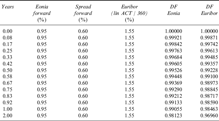
FRA = [L(1Y, 1Y) − 1.55%]PD (1Y, 1Y)
where L(1Y, 1Y) is the Euribor fixing in one year for a period of one year, discounted by the risk-free discount factor PD(1Y, 1Y).
We assume for simplicity a flat term structure of Eonia (risk-free) forward rates and a spread over it to determine 1-year Euribor-fixing forward rates. The data are shown in Table 7.19.
If the volatility of the Euribor fixing is 30% (it is supposed to be estimated from historical levels or based on market quotes of caps and floors), then we can derive ENE and PFE (at the 99% c.l.): they are shown in Table 7.20, which assumes the FRA has a notional of EUR1,000,000, for each corresponding date at the end of the 12 monthly survival periods into which we divide the duration of the contract. A visual representation is given in Figure 7.2.
The resulting LB at inception is EUR159,975, if we set the percentage of coverage at γ = 75% (it is computed using (7.25)). Investment of the LB in liquid assets (for β = 20%) and investment in liquid assets during each survival period are shown in Table 7.21, when the bank adopts ENE as a measure to predict negative exposures. If it chooses PFE, Table 7.22 shows the related liquidity buffer (computed using (7.26)) and the investment in liquid assets.
The LBCDC for both cases, expressed in absolute terms and as a percentage of the notional, are given in Table 7.23: they are computed using a funding spread level constant that is equal to sB = 1%. In both cases of ENE and PFE they are significant for the contract we are considering.
Table 7.20. ENE and PFE at the 99% confidence level at the end of monthly survival periods for the FRA
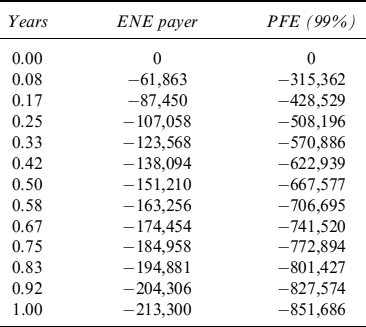
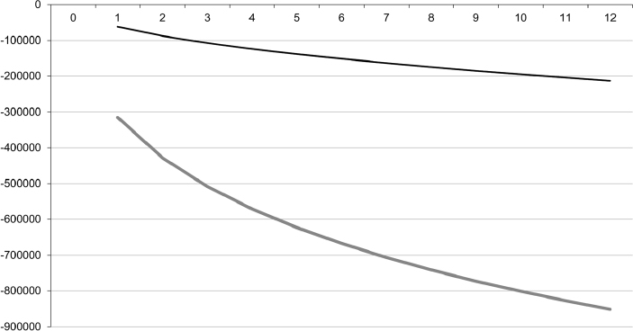
Figure 7.2. ENE (dark-grey line) and PFE (light-grey line) at the 99% confidence level at the end of monthly survival periods for the FRA
Table 7.21. Liquidity buffer evolution, fraction invested in liquid assets and investment in liquid assets during survival periods when ENE is used
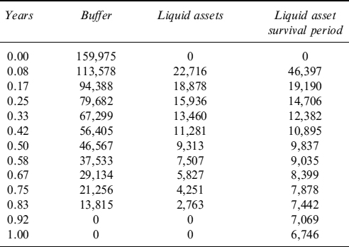
Table 7.22. Liquidity buffer evolution, fraction invested in liquid assets and investment in liquid assets during survival periods when PFE is used
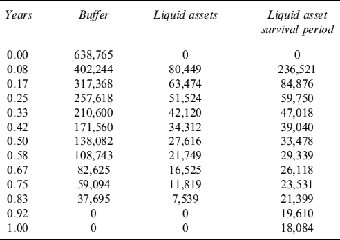
Table 7.23. Liquidity buffer costs in euros and as a percentage of the notional, when ENE or PFE is used
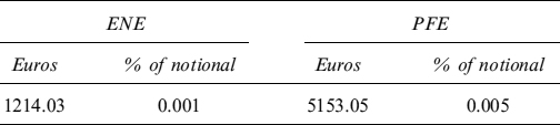
7.9 THE THIRD CAUSE OF THE LIQUIDITY BUFFER: OFF-BALANCE-SHEET COMMITMENTS
The presence of off-balance-sheet (OBS) commitments is another cause of the need for a liquidity buffer. In theory, there are many OBS commitments, including contingent financial obligations deriving from derivative contracts. For the limited scope of liquidity buffer needs, we can restrict our analysis to cases where financial guarantees are called for:
- standby letters of credit
- bank loan commitments
- note issuance facilities
More specifically, we analyse the case of bank loan commitments: they are promises made by the bank to a counterparty to grant a loan on some date in the future under certain conditions. We can identify the following types of bank loan commitments:
- Line of credit: This is an informal commitment by a bank to lend funds to a client firm.
- Revolving line of credit and committed credit lines: These are formal agreement by a bank to lend funds on demand to a client firm under the terms of a contract.
Although the first case is in theory easier to manage in terms of liquidity risk, in practice they both bring about liquidity needs and hence the necessity to plan a funding strategy and build a suitable LB to cope with unexpected events related to withdrawals by the counterparty.
Proposition 7.9.1. The liquidity buffer for a loan commitment is equal to its usage in excess, calculated at a given confidence level, with respect to expected usage by the counterparty.
Let us assume the bank commits to granting a loan, under given conditions, at any time the counterparty chooses in a period [T0, Tb], up to a maximum amount L. The counterparty can also choose not to ask for the loan. The bank expects usage to be equal to ![]() : in other words, the bank expects that the counterparty will ask to have a loan for an amount
: in other words, the bank expects that the counterparty will ask to have a loan for an amount ![]() . The bank also computes maximum usage at a given confidence level (say, 99%), such that a greater usage can only happen with a probability smaller than 1%: let U99 be such an amount. The bank can fund the commitment for average usage (as it would for a loan actually granted and not just a commitment) and can build a liquidity buffer for an amount equal to unexpected usage, defined as:
. The bank also computes maximum usage at a given confidence level (say, 99%), such that a greater usage can only happen with a probability smaller than 1%: let U99 be such an amount. The bank can fund the commitment for average usage (as it would for a loan actually granted and not just a commitment) and can build a liquidity buffer for an amount equal to unexpected usage, defined as:
LB(0) must of necessity be invested in cash or in liquid securities earning the risk-free rate r, since it will be needed when the counterparty asks for the start of the loan.
Proposition 7.9.2. The liquidity buffer cost for a loan commitment is proportional to the funding spread and to that part of the liquidity buffer not needed to cover unexpected usage.
The bank has to pay a funding spread on the sum it raises in the market to build the LB at the reference time. When the LB is not needed to cover unexpected usage then it is invested in liquid assets, so that the bank suffers a net cost equal to sB. On the other hand, if it is used to cover counterparty requests, it is reasonable to assume that the bank also included a charge for the funding spread in the contract terms, so that the expected return of the used amount is r + sB, thus producing a net cost equal to 0 for the bank. In conclusion, we can write the formula for liquidity buffer costs as:
Equation (7.29) states that liquidity buffer costs are equal to the funding spread sB applied over the period from T0 to Tb to all possible usages of the commitment below the 99% confidence level U99, but above the average level ![]() , with each case weighted by the probability of usage P[U]. In fact, when usage is at some level U above the expected level, but below the maximum usage at the predefined confidence level, then the bank has built an unnecessary buffer for an amount equal to the difference between the two levels. The cost to keep this buffer is given by the funding spread.
, with each case weighted by the probability of usage P[U]. In fact, when usage is at some level U above the expected level, but below the maximum usage at the predefined confidence level, then the bank has built an unnecessary buffer for an amount equal to the difference between the two levels. The cost to keep this buffer is given by the funding spread.
From equation (7.29) it is clear that the bank needs a model for usage of the credit line to assign a given probability to different levels of usage of the commitment. Such a model can be very complex when trying to capture real features of the behaviour of the counterparty linked to its creditworthiness and how it evolves in time. This is beyond the scope of the current analysis though; more in-depth analysis is postponed to Chapter 9, where we present a sophisticated stochastic model to manage the risks related to credit lines.
Remark 7.9.1. Equation (7.29) is based on several simplifying assumptions that need to be relaxed when building a realistic model for loan commitments. In fact, it is implicitly assumed that the counterparty chooses to use the line only once at the start of the commitment and then there is no further activity. In reality, if this behaviour can be reasonable for some kinds of commitments, in general it is not true because the counterparty can borrow money until the end of the commitment (within the limit of the notional amount obviously). Moreover, the possibility of having reimbursements during the life of the contract is not considered.
In conclusion, equation (7.29) should be seen as a rough first approximation to spot the main factors affecting the cost of the liquidity buffer for loan commitments.
Example 7.9.1. We show a credit line opened to a counterparty for a period of one year (so Tb = 1 and T0 = 1) with a maximum amount of 100. Possible usage levels of the line and associated probabilities are indicated in Table 7.24 and a visual representation is given in Figure 7.3.
Table 7.24. Usage levels of the credit line and associated probabilities
| Usage | P[U](%) |
| 0 | 20 |
| 22 | 21 |
| 42 | 22 |
| 61 | 20 |
| 81 | 16 |
| 100 | 1 |
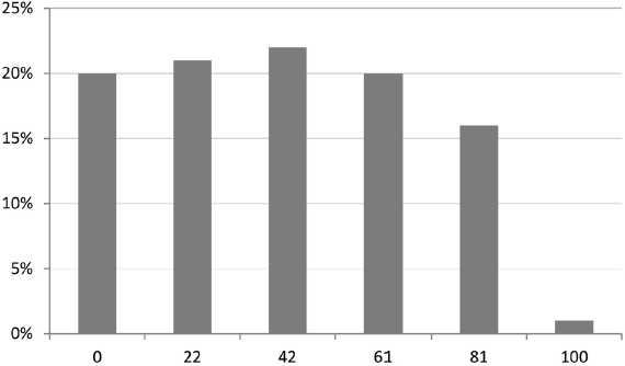
Figure 7.3. Usage levels of the credit line and associated probabilities
Table 7.25. Average usage, liquidity buffer and liquidity buffer costs as an absolute and as a percentage of the credit line amount
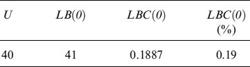
It is easy to compute expected usage, which is ![]() , and the maximum usage level at the 99% confidence level, which is U99 = 81, so that LB(0) = 41. Assuming the bank has a funding spread equal to sB = 1.5%, then LBCLC(0) can easily be computed by applying a discrete version of equation (7.29). Looking at this in greater detail, we have:
, and the maximum usage level at the 99% confidence level, which is U99 = 81, so that LB(0) = 41. Assuming the bank has a funding spread equal to sB = 1.5%, then LBCLC(0) can easily be computed by applying a discrete version of equation (7.29). Looking at this in greater detail, we have:
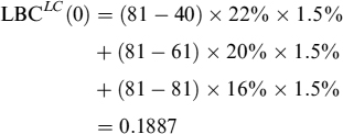
In Table 7.25 we recapitulate the results.
7.10 BASEL III REGULATION AND LIQUIDITY BUFFER
The document published by the Basel Committee in 2010 and amended in 2012 and 2013 (see [101] and [102]) introduced two main indicators to monitor and manage liquidity risk:15
- liquidity coverage ratio (LCR)
- net stable funding ratio (NSFR).
The LCR is important for impacts on the LB. It is defined as:
![]()
where
- HLA is the stock of high liquidity assets available to the bank: it includes cash and unencumbered Treasury bonds and corporate bonds that fulfil some criteria of low credit risk, ease and certainty of valuation, and low correlation with risky assets (this will exclude bonds issued by financial institutions from the stock).
- NCO is total net cash outflow occurring during a period of 30 days following calculation of the index; the outflow is defined as:
NCO = CF−(0, 30d) − min[CF+(0, 30d), 75% × CF−(0, 30d)]
where CF−(0, 30d) is the cumulated negative cash flow (i.e., the outflow) and CF+(0, 30d) is the cumulated positive cash flow (i.e., the inflow), over a period of 30 days starting from the reference date in 0.
In this section to hark back to Chapter 4 where we discussed in detail how to build the LCR.
The LCR aims at ensuring that the bank holds a sufficient buffer for liquidity needs in a short period of 30 days. The denominator of the ratio NCO measures net outflows occurring during the next 30 days whereas the numerator HLA identifies the quantity of liquid assets and cash (i.e., the liquidity buffer) that must be held. It is worth stressing that the LCR limits inflows to an upper bound given by 75% of the outflows, which basically means that the bank has to keep a liquidity buffer equal to 25% of the negative cumulated cash flows over the period of the next 30 days in any case.
The regulation does not indicate how the liquidity buffer has to be built or how it has to be funded: it just focuses on the need for an adequate amount capable to cover outflows in the next 30 days. Nevertheless, the bank needs a more forward-looking approach so as to preserve a value of the LCR above 1 in the future as well.
We have already outlined a framework to build the liquidity buffer and the term structure of funding such that the bank can be sure that there is liquidity equilibrium in the future, within the limits under which stressed scenarios were designed, when it operates usual financial intermediation activity. We would now like to analyse the possibility of fitting the same framework to regulatory requirements and specifically to the LCR, so that this ratio is ensured to be above 1 in the future as well.
First, the period of 30 days considered in the LCR corresponds to the survival period we mentioned above, so we can set τsv = 30/365: incidentally, this is what we have done in the examples in previous sections. Second, regulation prescribes a set of runoff factors to apply to different kinds of liabilities: they are the percentage of the expiring liability, or of the outstanding amount of NML assumed not to be renewed. The runoff factors are equivalent to the factors x% we used in our framework applied to the different liabilities.
The basic criterion used by the Basel Regulation to disentangle liabilities is based on the relationship between the bank and its creditors. Let us show a few instances in greater detail:
- Retail deposit runoff—
- Stable deposits (runoff rate = 3% and higher): In the framework we presented above the monthly withdrawal rate xNML% = 3% at least, which means that the minimum daily withdrawal rate is
 .
. - Less stable deposits (runoff rates = 10% and higher): the monthly minimum withdrawal rate xNML % = 10%, which amounts to a daily withdrawal rate of
 .
.
- Stable deposits (runoff rate = 3% and higher): In the framework we presented above the monthly withdrawal rate xNML% = 3% at least, which means that the minimum daily withdrawal rate is
- Unsecured wholesale funding runoff—
- Unsecured wholesale funding provided by small-business customers: 5% (stable funding), 10% (less stable funding) and higher; for these liabilities rollover risk is set in our framework at x% = 5% or x% = 10%.
- Unsecured wholesale funding with operational relationships: 25% (x% = 25%).
- Unsecured wholesale funding provided by non-financial corporates and sovereigns, central banks and public sector entities: 75% (x% = 75%).
- Unsecured wholesale funding provided by other legal entity customers: 100% (x% = 100%). The regulator specifies that “all notes, bonds and other debt securities issued by the bank are included in this category regardless of the holder, unless the bond is sold exclusively in the retail market and held in retail accounts, in which case the instruments can be treated in the appropriate retail deposit category.”
- Secured funding runoff—
- Loss of secured funding on short-term financing transactions: x% = 15% is the rollover risk assigned to funding backed by assets that in the numerator are considered to be Level 2; x% = 25% for secured funding transactions with the bank's domestic sovereign, domestic central bank, or domestic PSEs that have a 20% or lower risk weight, when the transactions are backed by assets other than Level 1 or Level 2 assets, in recognition that these entities are unlikely to withdraw secured funding from banks at a time of market-wide stress; finally, x% = 100% for all other maturing transactions.
- Additional requirements—
- Derivative payables: 100% runoff. Derivatives that expire in 30 days cannot be rolled over. This has not been considered in our framework since there is no liquidity buffer to set aside for this occurrence. LCR construction rules simply forbid compensating negative cash flows with positive cash flows of a corresponding new contract rolled over for another period.
- Increased liquidity needs related to downgrade triggers embedded in financing transactions, derivatives and other contracts: 100% of the amount of collateral that would be posted for or contractual cash outflows generated by any downgrade up to and including a three-notch downgrade. This has not been considered in the framework above, although it can easily be handled by an approach similar to that used to determine outflows due to collateralization of derivative contracts.
- Increased liquidity needs related to the potential for valuation changes on posted collateral securing derivative and other transactions (20% of the value of non-Level 1 posted collateral). This too has not been considered in the framework, but it can be handled using the modelling tools we introduce in Chapter 8.
- Loss of funding on asset-backed securities, covered bonds and other structured financing instruments and loss of funding on asset-backed commercial paper, conduits, securities investment vehicles and other such financing facilities. In both cases x% = 100%.
- Drawdowns on committed credit and liquidity facilities. The undrawn portion of existing facilities has to be included in outflows as follows:
- 5% drawdowns on committed credit and liquidity facilities to retail and small-business customers: At the inception of the contract the buffer should be computed on unexpected usage equal to ULCR = (1 − 5%)NL, where N is the number of months until the end of the contract. Then

 following the framework we presented above.
 - 10% drawdowns on committed credit facilities to non-financial corporates, sovereigns and central banks, public sector entities and multilateral development banks: In this case ULCR = (1 − 10%)NL and the liquidity buffer is computed accordingly.
- 30% drawdowns on committed liquidity facilities to non-financial corporates, sovereigns and central banks, public sector entities and multilateral development banks and 100% drawdowns on committed credit and liquidity facilities to other legal entities: In both cases
 , since the full amount beyond the average level has to be assumed withdrawn during the period.
- 5% drawdowns on committed credit and liquidity facilities to retail and small-business customers: At the inception of the contract the buffer should be computed on unexpected usage equal to ULCR = (1 − 5%)NL, where N is the number of months until the end of the contract. Then
- Increased liquidity needs related to market valuation changes on derivative or other transactions (non-0% requirement to be determined at national supervisory discretion): We can use in this case the approach sketched in Section 7.8, setting γ equal to the level decided by national authorities.
There are some other minor contingent outflows we have not included in the list, but can be included under a conceptual point of view in one of the cases above.
Following our approach to build the term structure of funding based on rollover (runoff) risk factors, it should be noted that bonds usually issued by banks in the market cannot be used to fund assets with expiries longer than their own. This is not strictly forbidden by regulation, but we showed that should a bank want to follow an equilibrium liquidity policy established since the beginning of the reference date, then a rollover risk factor x% = 100% implies that available liquidity beyond the expiry of the liability is nil. In practice, the LCR implicitly forbids any maturity transformation activity insofar as liabilities with a runoff factor of 100% are concerned.
Regulation does not forbid non-equilibrium policies either, so that in theory the bank could follow a strategy like that described in Section 7.5 to fulfil the requirement that LCR ≥ 1. In practice, the bank can fund its LB in an inconsistent (according to our analysis) way relying on the low probability of occurrence of stressed scenarios. When this happens, though, it is much more likely that the LB is less effective to protect the bank.
In the following chapters we present models that enable the bank to simulate the main items on its balance sheet: this makes it possible to better manage and monitor the effectiveness of the LB. Moreover, it is possible to simulate the evolution of the LCR both for regulatory or risk management purposes as well.
1 This means the bank accepts a 1% probability of failing under more stressed liquidity conditions, which eventually may produce bankruptcy because an insufficient liquidity “hedge” has been set up.
2 Note that we are simply showing the total cash flows that originated on the first rollover date; we are not presenting a formula predicting future cash flows.
3 See Chapter 10 for a discussion on the interrelations between credit, funding and liquidity.
4 There is the assumption here that the spread sA is set in such a way that it also compensates for the loss on the spread sB in case of default by the counterparty. Equation (7.3) can easily be modified to include this effect as:
![]()
5 The assumption can easily be relaxed although it would make the notation much heavier, without adding deeper insight to the analysis.
6 In what follows we indicate the actual size of the buffer or the actual amount of buffer costs by an asterisk “*”, whereas the same quantities without any sign indicate the value predicted at time T0 should a stressed scenario occur.
7 In the present setting, since the risk-free rate is constant, PD(0, T) = e−r*×T, where r* = ln(1 + r).
8 Recall that this part of the LB is determined by the preference parameter for liquid investments β we introduced above.
9 In Chapter 9 we will introduce a behavioural model that allows the future probability distribution of deposit volumes to be determined. It is then possible to exploit the distribution to set the implied xm% after a suitable confidence level is chosen (say, the lowest level of volumes at the 99% c.l.).
10 Normally, creditors financing via sight deposits are termed “clients” by the bank.
11 The same considerations on the nature and meaning of x% for a standard maturing liability can also be applied to xNML%.
12 In this case a haircut on the market price is applied and the resulting value is considered equivalent to cash. We do not deal with these aspects here, but they have to be properly considered for full evaluation of the costs related to the liquidity buffer. See Chapter 8 for a possible solution on how to model haircuts.
13 This is consistent with the standard CSA agreements and collateral rules of clearing houses, whereby the agent posting collateral receives the OIS (Eonia for the Euro) rate, which is assumed to be the best approximation to a risk-free rate, and is the market remuneration rate for an unsecured investment of money on a one-day time horizon in any case.
14 Basically, for the fraction β invested in liquid assets and the amount posted as collateral, the gain equal to the risk-free rate compensates only the risk-free part of the funding cost on the debt, leaving the bank with the net cost equal to the funding spread.
15 See also Chapter 4 for an extensive discussion on the subject.