
9.1 INTRODUCTION
Some items on the balance sheets of banks need to be modelled by a behavioural approach. By “behavioural” is generally meant a model that takes into account not only standard rationality principles to evaluate contracts, which basically means that economic agents prefer more wealth to less wealth, and that they prefer to receive cash sooner than later; behavioural models consider other factors as well, typically estimated by means of statistical analysis, which may produce effects that otherwise could not be explained. It should be stressed that in any event financial variables, such as interest rates or credit spreads, are the main driver of customer or, more generally, counterparty behaviour.
There are three main phenomena that need behavioural modelling: prepayment of mortgages, evolution of the amount of sight and saving deposits and withdrawals from credit lines. We will propose models for each focusing mainly on what we think is a good solution for liquidity management, without trying to offer a complete picture on the entire range of available models developed in theory or in practice. Anyway, as far as mortgage prepayments and withdrawals from credit lines are concerned, we introduce models that to our knowledge have never been proposed before, which aim at considering financial, credit and liquidity risk in a unified framework.
9.2 PREPAYMENT MODELLING
The prepayment of mortgages has to be properly taken into account in liquidity management, although many of the effects of the decision to pay back the residual amount of debt by the mortgagee are financial as they may cause losses to the financial institution. We will present a model to cope with the prepayment of fixed rate mortgages, because they combine both liquidity and financial effects.
9.2.1 Common approaches to modelling prepayments
There are two fundamental approaches to model prepayments
- Empirical models (EMs): Prepayment is modelled as a function of some set of (non-model based) explanatory variables. Most of these models use either past prepayment rates or some other endogenous variables (such as burnout) or economic variables (such as GDP or interest rate levels) to explain current prepayment. Since they are just heuristic reduced-form representations for some true underlying process, it is not clear how they would perform in a different economic environment. Besides, no dynamic link between the prepayment rate and other explanatory variables has been established.
- Rational prepayment models (RPMs): They are based on contingent claims pricing theory and as such the prepayment behaviour depends on interest rate evolution. Prepayment is considered as an option to close the contract at par (by repaying the nominal value of the outstanding amount), which will be exercised if the market value of the mortgage is higher than the nominal residual value. Although these models consistently link valuation of the mortgage and prepayment, their prepayment predictions do not closely match observed prepayment behaviour since not all debtors are skilled enough to evaluate the convenience of exercising the options. One of the drawbacks of rational models is that in their basic forms they imply that there will either be no prepayment or all mortgages with similar features will suddenly prepay, because all mortgagees will exercise their options.
Empirical features commonly attributed to mortgage prepayment are the following:
- some mortgages are prepaid even when their coupon rate is below current mortgage rates;
- some mortgages are not prepaid even when their coupon rate is above current mortgage rates;
- prepayment appears to be dependent on a burnout factor.
Since basic and simple RPMs are unable to fully take into account these features, most banks adopt EMs in an attempt to accurately predict prepayment rates. The prediction is the so-called CPR, or constant prepayment rate, which is used to project expected cash flows and which can be expressed as a function of different variables. For example, a well-known EM is the Richard and Roll [105] model adopted by Goldman Sachs and the US Office of Thrifts and Supervision; this model can be written in very simple form as:
CPR = f(Refinance incentive)g(Seasoning)h(Month)l(Burnout factor)
So the CPR depends on four functions of four different factors, the most important of which happens to be the refinance incentive or, in other words, exercising the option when it is convenient to do so. The refinance incentive (RI) function f() is modelled as:
RI = 0.3124 − .020252 × arctan(8.157[−(C + S)/(P + F) + 1.20761])
where arctan is the arctangent function, C is the fixed rate of the coupon, S is the servicing rate of the pool,1 P is the refinancing rate and F are additional costs due to refinancing.
In general, EMs perform quite well when predicting expected cash flows; they are also used to set up portfolios with hedging instruments with the notional adjusted according to the CPR. Since most model vendors plug EMs into their ALM systems and most banks use them, we examine how hedging with EMs works in practice.
9.2.2 Hedging with an empirical model
The refinance incentive is the most important factor, particularly in market environments with extremely low rates. In some countries mortgagees are charged no prepayment penalties, so they are more eager to exploit the prepayment option. Moreover, some regulations allow mortgagees to transfer the mortgage to another bank at no cost: in this case competition amongst banks pushes the refinancing of mortgages with high contract rates when rates are low, thus increasing the “rationality” of prepayment. Even if the bank manages to keep the mortgagee, it is forced to refinance the mortgage at new market rates. In either case, in practical terms this is equivalent to a prepayment.
It goes without saying that, when the refinancing incentive is the major driver for prepayments, the bank suffers a loss that in very general terms can be set equal to the replacement cost of the prepaid contract.
For this reason we introduce a very simplified EM, and we use a function of the kind:
where C and P are defined as above. The CPR in equation (9.1) is a constant α plus a proportion β of the ratio between the mortgage rate C and the current rate level P. The lower the current rate P, the higher the CPR.
Let us create a laboratory environment and calibrate model (9.1) to empirical data reproduced by a random number generator. We assume that P is representative of a “general” level of interest rates (e.g., the average of the 5, 10 and 20-year swap rates). Moreover, C is the average fixed rate of the portfolio of mortgages, which we set equal to 3.95% (in line with the market rates we consider below). For each level of rates we have an annual CPR generated by the equation:
![]()
where ![]() is a random number extracted from a normally distributed variable. The data are shown in Table 9.1.
is a random number extracted from a normally distributed variable. The data are shown in Table 9.1.
We carry out linear regression to estimate the parameters and get α = 0.02881267 and β = 0.029949414. A graphical representation of the fitting is given in Figure 9.1.
The simple model above seems able to capture the relevant factors affecting prepayment activity, which is strongly dependent on the level of the current interest rate. Given this, we have the CPR to project expected cash flows and then to set up proper hedging strategies with other interest rate derivatives, typically IR swaps. The main problem with such an EM is that it is not dynamic and, unfortunately, does not allow for an effective hedge against both movements in interest rates and prepayment activity.
Table 9.1. Current level of rates P, ratio between fixed mortgage rate and current level of rates (C/P) and percentage of prepaid mortgages PP%
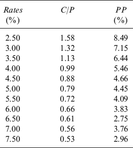
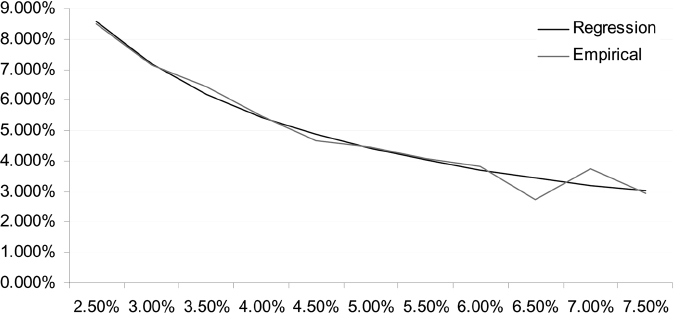
Figure 9.1. Linear regression estimation of prepayment data. The percentage of prepayments in one year is plotted against the current interest rate level
To see this, let us consider a mortgage that is representative of a bank's mortgage portfolio sold to clients at current market conditions. The mortgage expires in 10 years, it is linearly amortizing and its fair fixed rate, yearly paid, is 3.95%, given the 1Y Libor forward rates and associated discount factors shown in Table 9.2. In Table 9.3 the oustanding capital at the beginning of each year is shown. For simplicity's sake we also assume that no credit spread is applied, nor any markup to cover administrative costs, so that the mortgage rate is given only by Libor rates.
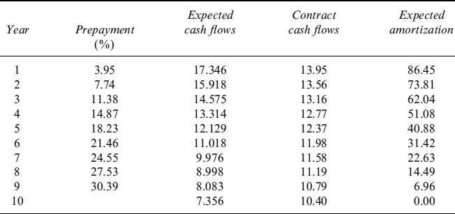
We can also compute expected cash flows given the prepayment activity forecast by the model we calibrated. If we assume that the current level of the interest rate is summarized in the 10Y rate, 5.5%, the model provides a CPR of 4.02% p.a. Expected amortization and contract and expected cash flows are easily computed (see Table 9.4). In computing expected cash flows we used the convention that the CPR is a continuous rate such that, for a given year T, the percentage of prepaid mortgages is (1 − e−CPR×T).
Table 9.2. 1Y Libor forward rates and discount factors for maturities from 1 to 10 years
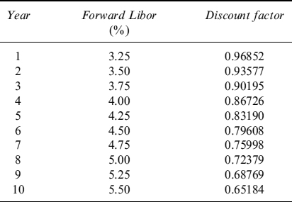
Table 9.3. Outstanding capital at the beginning of each year for the representative mortgage
| Year | Outstanding capital |
| 1 | 100 |
| 2 | 90 |
| 3 | 80 |
| 4 | 70 |
| 5 | 60 |
| 6 | 50 |
| 7 | 40 |
| 8 | 30 |
| 9 | 20 |
| 10 | 10 |
The mortgage rate computed on expected cash flows, keeping in mind the prepayment effects, is slightly lower and equal to 3.89%. This is easy to understand, since we are in a steep-curve environment and the prepayment entails a shorter (expected) maturity of the contract, thus making the fair rate lower. In a very competitive market, it is tempting for the bank to grant such a lower rate to mortgagees, because after taking account of the costs related to hedging the bank appears not to be actually giving away value to customers.2
In fact, the ALM of the bank typically finances the mortgage portfolio by rolling over short-term debt or a similar maturity debt, but at a floating rate. The reason is easily understood, since as a result of floating rate indexation the duration of the bank debt is very short, and hence the volatility of balance sheet liabilities is reduced as well. As a consequence, the bank transforms its fixed rate mortgage portfolio into a floating rate mortgage portfolio (so that asset duration matches liability duration),3 by taking expected cash flows instead of contract cash flows into account: in this way risk managers believe they have appropriately hedged prepayment risk as well, at least in average terms. The transformation, or hedge, is performed using liquid market instruments, usually swaps, by paying the fixed rate earned on the mortgage and receiving the Libor fixing (which is concurrently paid on financing).
In the example we are considering, the swap used for hedging purposes is not standard, but an amortizing swap with a decreasing notional equal to expected amortization as shown in the fourth column of Table 9.4, which reveals expected outstanding capital at the end of each year. Since we are not considering any credit spread on the mortgage, and assuming no credit issues in the swap market as well, we get the swap fair rate at inception as 3.89%, which is exactly the mortgage rate computed using expected (i.e., including the prepayment effect) cash flows, hence confirming that none of the hedging costs have been ignored when pricing the mortgage out of expected cash flows instead of contract cash-flows.
Table 9.4. Percentage of prepaid loans up to a given year, expected and contract cash flows and expected amortization
If the model is correctly predicting prepayment rates, then there would be no loss: at the end of each year the outstanding capital matches the expected capital (net of prepayments) and the hedging swap would still be effective in protecting against exposure to interest rate movements. The problem is that the very model we are using (which, we recall, is a simple version of the most common models included in the ALM applications of software vendors) actually links the level of the CPR to the level of interest rates. So, barring possible divergences due to normal statistical errors, variations in the CPR are also due to movement in the term structure of interest rates, although this cannot be dynamically included in risk management policies since the EM is static. If rates move, this means that swap hedging will no longer be effective and the bank will have to appropriately rebalance its notional quantities. But, interest rates do move, so we can be sure that the hedge has to be rebalanced in the future, even if the estimated parameters of model (9.1) prove to be correct and do not change after a new recalibration.
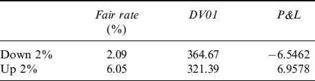
Being pretty sure that the bank will change the notional of the hedging swap in the future, the problem is now to understand if this rebalancing generates a loss or a profit (without considering transaction costs). Let us see what happens if the term structure of forward rates experiences a parallel shift downward or upward of 2% after 1 year. In this case, if the probabilities of prepayment are kept constant, the hedging swap portfolio would experience a positive, or negative, variation of its net present value (NPV), thus counterbalancing the negative, or positive, variation of the NPV suffered on the mortgage. The profit, or loss, can be approximated with very high accuracy, since we are assuming a parallel shift of the forward rates that would be equal to DV01 × Δr, where DV01 is the discounted annuity of fixed rate payments of the swap, and Δr is variation of the swap fair rate due to the change in Libor forward rates.
In Table 9.5 we show the profit and loss due to unwinding of the original hedging swap for the two scenarios of parallel shift (upward and downward) of the forward rate term structure. When rates fall, the hedging swap suffers a loss, since it is a (fixed rate) payer and the new fair rate for a similar swap structure is 2.09%; the loss is given by the DV01 indicated in the second column times the Δr = 2.09% − 3.89%. On the other hand, when forward interest rates move upward by 2%, the unwinding of the swap generates a profit, computed as before considering the new fair swap rate 6.05%. As expected, the profit has the same order of magnitude as the loss. Moreover, since the swap is mimicking the mortgage, variation of the NPV of the latter is a mirror image of the former. The reason we have to unwind the original hedging swap and open a new one will be clear in what follows.
Table 9.5. Profit and loss due to closing of the original hedging swap position
Actually, if the probabilities of prepayment change according to (9.1), we have two consequences: first, the original swap no longer perfectly hedges variations in the value of the mortgage; second, rebalancing of the notional of the swap is needed at least to bring it back into line with the new expected amortization schedule of the mortgage. We have then to unwind the original position and open a new one with a new swap with a notional amount matching the expected amortization schedule of the mortgage, with a fixed rate equal to the mortgage rate based on current market rates.4
First, let us examine what happens to expected repayments in the future when rates move. Table 9.6 shows the new expected amortization schedule after a change in the CPR due to a movement in interest rates: with a new level of the 10Y5 at 3.5%, the CPR would be 8.49%. This means that the actual outstanding capital after one year will be less than that projected by the starting CPR (4.02%), and consequently future expected outstanding capital amounts will also be smaller (i.e., the expected amortization will be more accelerated).
The same reasoning also applies to a scenario where the term structure of forward rates experiences a shift upward of 2%, as shown in Table 9.7. In this case, from (9.1), we know that the new CPR rate will be 2.96%, in correspondence with the 10Y forward rate of 7.50%. Hence the oustanding amount after one year will be higher than the one previously projected, and thus all expected future capital amounts will also be revised upward (i.e., amortization will be slower).
We now have to compute the profit or loss produced by opening a position in a swap with the same rate as the original one (which is also the mortgage rate that we need to match on interest payment dates), with a reference capital schedule mirroring the revised expected amortization of the mortgage at current market rate levels. Table 9.8 summarizes the results for both scenarios. When rates are down 2%, the new swap generates a profit of 4.7119: this is easy to understand, since the bank still pays 3.89% on this contract, although the new fair swap rate is 2.37% (the profit is computed as above by means of the DV01 in the second column). Nevertheless, keeping the loss incurred in mind when closing the original swap position, the bank suffers a total net loss of −0.8185 (shown in the fourth column).
Table 9.6. New expected amortization schedule after the term structure of forward rates drops 2%. The CPR moves from 4.02 to 8.49% according to model (9.1)
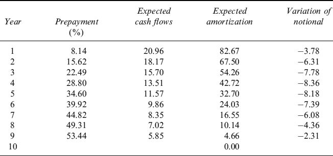
Table 9.7. New expected amortization schedule after a shift upward for the term structure of forward rates of 2%. The CPR moves from 4.02 to 2.96% according to model (9.1)
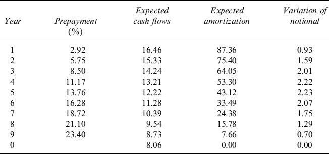
Table 9.8. Profits and losses due to the opening of new hedging swaps and the net result of closing the original position
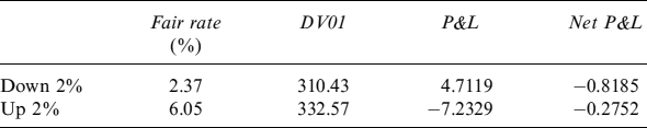
Surprisingly enough, a net loss is also suffered by the bank when prepayment activity slows down as a result of higher rates in the upward parallel shift scenario. Actually, notwithstanding the profit gained when closing the original swap position, the loss suffered when opening the new swap is even higher.
At this point we can be pretty certain that, unfortunately, the hedging strategy of a mortgage, based on taking a position in swaps with a notional schedule mimicking the mortgage's expected amortization, is flawed and produces losses unless rates do not change and consequently the CPR is fixed too. In reality, this rarely happens since interest rates move and EMs predict changing CPRs. We need to investigate further where the losses come from, so that we can hopefully come up with a more effective hedging strategy.
9.2.3 Effective hedging strategies of prepayment risk
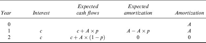
To better understand how losses are produced when hedging expected cash flows, we consider the following case: a bank has a bullet mortgage with a mortgagee of amount A, which expires in two years. At the end of the first year the mortgagee pays fixed rate interest c and at the end of the second year she repays interest c and capital A. At the end of the first year, she also has the option to prepay the entire outstanding amount plus the interest accrued up to then: we assume that this option is exercised with probability p. Table 9.9 shows expected cash flows and expected and contract amortization at the beginning of each year.
Table 9.9. A simple 2-year bullet mortgage
The bank closes a (fixed rate) payer swap with 2-year expiry and varying notional amount equal each year to the expected amortization. This is not a standard swap traded in the interbank market, but it is not difficult to get a quote on it by a market maker. Let us indicate by Swp(n, m) a swap starting at time n and expiring at m. We can decompose the 2-year swap in two single-period swaps, so that the hedging swap portfolio P is comprised of:
- A × Swp(0, 1)
- (A − A × p) × Swp(1, 2)
It is very easy to check that the portfolio is
P = A × Swp(0, 2) − p × A × Swp(1, 2)
since Swp(0,1) + Swp(1,2) = Swp(0,2). The second component of the portfolio is a short position in a forward starting swap, whose notional is the mortgage notional amount weighted by the probability of prepayment at the end of the first year. The forward starting swap can be further decomposed, by means of put–call parity, as follows:
Swp(1, 2) = Pay(1, 2; c) − Rec(1, 2; c)
where Pay(n, m; K) (Rec(n, m2; K)) is the value of a payer (receiver) swaption struck at K, expiring at n, written on a forward swap starting at n and maturing at m. So, collecting results, we have that the hedging portfolio is:
If the probability of prepayment p (the CPR approximately in practice) is invariant with the interest rate level,6 equation (9.2) is just an alternative way of expressing a position in a swap with maturity and amortizing notional equal to that of the mortgage. So, the following two strategies are exactly equivalent:
- Entering in a (fixed rate) payer swap, with an amortizing schedule equal to the mortgage's expected amortizing schedule, and with the same expiry as the mortgage.
- Entering in a (fixed rate) payer swap, with a amortizing schedule equal to the mortgage's contract amortizing schedule, and with the same expiry as the mortgage; selling a payer swaption expiring in one year and written on a one-year swap, struck at the mortgage rate level c; buying a receiver swaption, otherwise identical to the payer swaption. The amount of the swap underlying the swaptions follows the contract amortizing schedule, whereas the quantity of swaptions to buy, or sell, is equal to the prepayment probability.7
Any equivalence between strategies (1) and (2) vanishes if the probability of prepayment p is not independent of the interest rate level, as is also the case in the very simple EM we presented in the previous section and generally the case in reality. If this is the case, decomposition allows for a more precise and effective hedge, provided we design a model capable of encompassing all these aspects.
Returning to our numerical example in the section above, it is now quite simple to understand the factors causing losses. In fact, in the numerical example the bank has decided to hedge the mortgage by strategy(1), assuming there is constant probability of prepayment (CPR). But the behaviour of the mortgagee (modelled via EM (9.1)) implies a higher probability when rates go down and lower when they go up. We can make the following points:
- When interest rates fall, the mortgage's NPV increases, and this is compensated by the payer swap with the same maturity. The loss originates from the fact that the probability of prepayment is higher than that guessed at the contract's inception. When seen from the perspective of strategy (2), it is as if the bank had bought a receiver swaption whose quantity is the probability of prepayment assumed at the beginning of the contract, but this is not enough to cover the loss of the mortgage which implies being short a receiver swaption with a larger quantity equal to the new prepayment probability.
- When interest rates rise, the mortgage's NPV decreases, this being counterbalanced by an increase in the swap value. In this case the loss also originates from the fact that the short position in the payer swaption (equal to the starting probability of prepayment) turns out to be bigger than that needed by the lower prepayment probability concurrent with higher rates.
- A more general point relates to why a bank should also sell the payer swaption when hedging the mortgage? When the bank adopts strategy (1), it is implicitly replicating the short position in the payer swaption, with the even worse circumstance of doing so in a higher than needed quantity when its NPV is negative (i.e., when rates move upwards). Actually, if the bank adopts hedging strategy (2), it is able to disentangle the different instruments to be bought or sold, and then to decide which is worth trading or not.
The analysis in this section is very useful and in Appendix 9.A we break down the hedging portfolio for a generic mortgage with a given expiry and amortizing schedule. In summary, the hedging portfolio comprises:
- A payer swap with the same fixed rate and expiry as the mortgage, and with the same amortizing schedule as the mortgage's contract amortization schedule.
- A short position in a portfolio of payer swaptions, expiring on each repayment date and written on a swap whose maturity date is the same as the mortgage's and as the mortgage's contract amortization schedule.
- A long position in a portfolio of receiver swaptions, expiring on each repayment date and written on a swap whose maturity date is the same as the mortgage's and as the mortgage's contract amortization schedule.
Each swaption has a quantity equal to the probability that prepayment occurs between the expiry dates of two contiguous swaptions.
Important implications can be drawn from the hedging portfolio:
- To properly hedge prepayment risk, a dynamic model of prepayment probability has to be designed, so as to allow for an increase in prepayments when rates go down.
- Making the probability higher when rates are low increases sensitivity to the value of the receiver swaptions that the bank has to buy to hedge the exposure. This yields more reliable hedging ratios and allows appropriate hedging against the costs incurred when prepayment activity increases.
- Moreover, making the probability higher when rates are low increases the price of the receiver swaption portfolio needed to hedge the exposure. This means that prepayment options are priced more accurately and can be included in the final rate to apply in the mortgage's contract.
- Selling the payer swaption portfolio is not needed: doing so unnecessarily offsets a mirror image long-option position on the mortgage that can grant some profits. We have seen that the standard strategy and other commonly adopted strateges do indeed mimic the selling of this swaption portfolio, very likely by an overdue amount.
- When including the effects of prepayments in the pricing of the loan, the bank does not have to price the long position in the payer swaption portfolio, which reduces the final contract rate. In fact, this is an obscure optionality that cannot easily be priced by mortgagees, even in a very competitive environment with rather sophisticated players.
9.2.4 Conclusions on prepayment models
Some recipes can be provided for the design of a prepayment model:
- EMs can be useful, but they have to be integrated with a RPM: the decomposition shown above makes it clear that mortgagees are implicitly long a portfolio of receiver swaptions by a certain amount that has to be included in the pricing.
- Probabilities of prepayment must be dynamically linked to the level of interest rates.
- Since we need to include the valuation of options in the pricing, we need also to account for the volatility of interest rates, so that a prepayment model has to be designed jointly with an interest rate model.
- As a consequence we can hedge sensitivities not only to interest rates, but also to volatilities (i.e., Vega).
In Section 9.2.5, we develop a prepayment model8 to hedge the prepayment risk of fixed rate mortgages which considers all the points above. It provides the ALM with a valuable tool to embed the costs of implied optionalities in the pricing of new mortgages, and to effectively hedge the exposures of an aggregated mortgage portfolio.
Undertaking the computation is a formidable challenge, so we come up with an accurate and quick solution that avoids resorting to Monte Carlo valuations, which are rather unstable when computing sensitivities and not suitable for a portfolio of hundred of thousands of contracts such as bank mortgage portfolios.
9.2.5 Modelling prepayment decisions
Assume that a bank closes a number of fixed rate mortgage contracts with clients who have the possibility to prepay the outstanding debt balance in the future. Further assume that mortgagees decide whether to prepay their mortgage at random discrete intervals, usually clashing with payment dates. The probability of a prepayment decision taken on the basis of the interest rate level is described by hazard function λ: the probability that the decision is made in a time interval of length dt is approximately λdt. Basically, this decision is taken when interest rates fall.
Besides prepayment (refinancing) for interest rate reasons, mortgagees may also prepay for exogenous reasons (e.g., job relocation or house sale). The probability of exogenous prepayment is described by hazard function ρ: this represents a baseline prepayment level (i.e., the expected prepayment level when no financially optimal (interest-driven) prepayment should occur).
We model the interest rate based prepayment within a reduced-form approach. This allows us to include prepayments in the pricing, interest rate risk management (ALM) and liquidity management consistently. We adopt a stochastic intensity of prepayment λ, assumed to follow CIR dynamics:
![]()
This intensity provides the probability of the mortgage rationally terminating over time. We further assume that the intensity is correlated to interest rates, so that when rates move to lower levels, more rational prepayments occur: this stochastic framework allows for a wide variety of prepayment behaviours. Survival probability (i.e., the probability that no rational decision is taken up to time T, evaluated at time t) is:
Functions A(t, T) and B(t, T) are given in equation (8.69). Parameter ψ is the market premium for prepayment risk and is assumed to be 0.9
Exogenous prepayment is also modelled in reduced-form fashion by constant intensity ρ: it can actually be time dependent as well. In this case the survival probability, or the probability that no exogenous prepayment occurs up to time T, evaluated at time t, is:
Total survival probability (no prepayment for whatever reason occurs) is:
whereas total prepayment probability is:
Consider a mortgage with a coupon rate c expiring at time T. At each period, given current interest rates, the optimal prepayment strategy determines whether the mortgage holder should prepay and refinance at current rates. Loosely speaking, for a given coupon rate c, keeping transaction costs in mind, there is a critical interest rate level r* such that if rates are lower (rt < r*) then the mortgagee will optimally decide to prepay. If it is not optimal to refinance, any prepayment is for exogenous reasons; otherwise, the mortgagee may prepay either for interest rate related or for exogenous reasons.
In order to make the model more analytically tractable, we assume that both types of decisions10 may occur at any time, but the effects on prepayments by the rational decision are produced only when the rates are below critical levels. In other words, when a rational decision is taken and the rates are above critical level r*, no prepayment actually occurs and no cost is borne by the bank. For such a mortgage, the rational decision produces no effects and cannot be taken again in the future, since both rational and exogenous decisions may occur only once, and as soon as one of the two occurs the mortgage is prepaid.
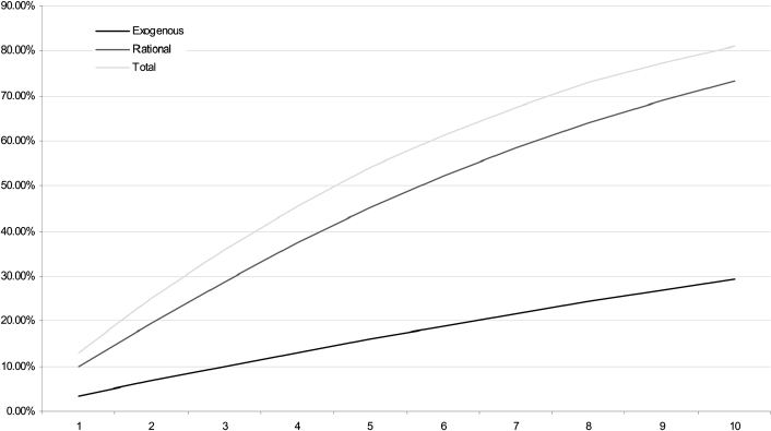
Figure 9.2. Rational and exogenous prepayment probabilities for a 10-year mortgage
Example 9.2.1. Figure 9.2 plots prepayment probabilities for different times up to (fixed rate) mortgage expiry, assumed to be in 10 years. The three curves refer to:
- exogenous prepayment, given by constant intensity ρ = 3.5%;
- rational (interest-driven) prepayment, produced assuming λ0 = 10.0%, κ = 27±%, θ = 50.0% and ν = 10.0%.
- total prepayment, when it is rational to prepay the mortgage (rt < r*).
9.2.6 Modelling the losses upon prepayment
Assume at time t0 the mortgage has the following contract terms:
- the mortgage notional is A0 = A and the mortgagee is not subject to credit risk;
- the mortgagee pays at predefined scheduled times tj, for j ∈ (0,1,…, b), a fixed rate c computed on the outstanding residual capital at the beginning of the reference period Tj = tj − tj−1, denoted by Aj−1. The interest payment will then be cTjAj−1;
- on the same dates, besides interest the mortgagee also pays Ij, which is a portion of the outstanding capital, according to an amortization schedule;
- the expiry is time tb = T;
- the mortgagee has the option to end the contract by prepaying on payment dates tj the remaining residual capital Aj, together with the interest and capital payments as defined above. The decision to prepay, for whatever reason, can be taken at any time, although the actual prepayment occurs on scheduled payment dates.
The assumption that the interest, capital, and the prepayment dates are the same is easily relaxed.
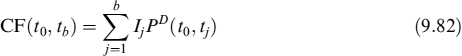
The fair coupon rate c can be computed by balancing the present value of future cash flows with the notional at time t0:
![]()
which immediately leads to:
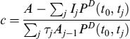
where PD(t0, tj) is the discount factor at time t0 for date tj. It should be noted that the quantity A − ∑jIjPD(t0, tj) can be replaced by ∑jTjAj−1Fj(t0)PD(t0, tj),11 where Fj(t0) is the forward rate at time t0 starting at time tj.
Assume now that the mortgage is prepaid at a given time tk (for k ∈ {0,1,…, b}); its current value will be:
![]()
where AP will almost surely be different from the residual capital amount Ak−1, unless the forward rates implied in the term structure at time t0 actually occur in the market at time tk. The prepayment can be either rational or exogenous.
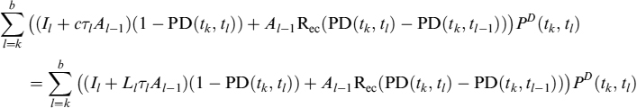
After prepayment, to hedge its liabilities the bank closes a new mortgage similar to the prepaid one, so that this new one replaces all previous capital payments and yields new interest rate payments as well. The fair rate ck,b(tk) of this new mortgage12 will be determined by market rates at time tk:
![]()
Hence, the bank will suffer a loss or earn a profit given by:
The bank is mainly interested in measuring (and managing) expected losses relating to the (rational) prepayment at times {tk}, which we indicate as expected loss (EL) evaluated at time t0:

Equation (9.8) can be computed under the forward mortgage rate measure Qk,b (where Q is the real measure), associated with the rate ck,b(tk), as:

The numeraire under this measure is ∑jPD(tk, tj)TjAj−1.
EL is a function of the term structure of risk-free rates.13 We model risk-free rates in a market model framework:14 each forward rate is lognormally distributed, with a given volatility that can be estimated historically, or extracted from market quotes for caps and floors and swaptions:
dFj(t) = σjFj(t)dWt
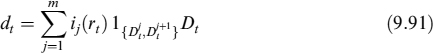
Any prepayment causing a loss for the bank can be caused for both exogenous and rational reasons, such an occurrence is described by intensity λt: we assume that this intensity is negatively correlated to the level of interest rates. There is also a contribution arising from exogenous prepayment decisions, which may occur under any market condition, thus generating either a loss or a profit to the bank. It is then possible to compute the expected loss on prepayment (ELoP), defined as expected loss at time tk when the decision to prepay (for whatever reason) is taken between tk−1 and tk:

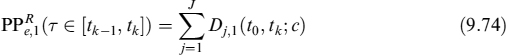
where 1T∈[tk−1, tk] is the indicator function equal to 1 when prepayment occurs within period of time [tk−1, tk]. Under the forward mortgage rate measure Qk,b we have

Valuation of the EL
From (9.8) the EL at time tk can easily be seen as the (undiscounted) value of a swaption written on a non-standard swap. A closed-form approximation for such contracts has been derived by Castagna et al. [49].
Let us start with a standard swaption (i.e., a swaption written on a standard swap). The fair swap rate at inception of the contract is:

where τi is the year fraction between Ti−1 and Ti fixed rate payment dates, and PD(t, T) is the price of a zero-coupon bond at time t expiring at time T. The rate is derived by setting the value of the swap at the start of the contract at zero:
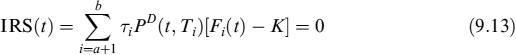
where Fi(t) is the forward risk-free rate
![]()
We denote by Swpt(t, s, Tb, S(t; s, Tb), K,σs, Tb, ω) the value of a swaption at time t, expiring in s and struck at K, written on a forward swap rate S(t; s, Tb); this value is calculated by the standard market (Black) formula with implied volatility σs, Tb, and the last argument indicates whether the swaption is a payer (1) or a receiver (−1). The formula is:
The formula can be found in Section 8.3.9. We have used the notation Ca,b(t) for an annuity that is equal to:
In the specific case of a non-amortizing mortgage of notional A, with fixed rate payments on dates {tk}, starting at tk and ending at Tb, the fair coupon rate can easily be shown to be equal to the fair swap rate, so ck, b(t0) = Sk,b(t0). This has to be compared with the original mortgage rate c (relating to a similar mortgage that started at t0, see equation (9.7)), so the expected loss on prepayment dates {tk} is:
Typically mortgages are amortizing, so we need a formula to price non-standard swaptions. We use the term “meta-swap” for a swap with unit notional and a time-varying fixed rate that is equivalent to the contract fixed rate times the notional amoun for each date ![]() (i.e., the one at the start of the calculation period).
(i.e., the one at the start of the calculation period).
Let us assume that the IRS floating leg pays at times Ta,…, Tb, where Ta is the first payment time after the EL time tk, and that the IRS fixed leg pays at times Tc1,…, TcJ, where c1 ≥ a and cJ = b (fixed leg times are assumed to be included in the set of floating leg times, and in reference to a mortgage they will be assumed to be the same for both legs).
The fixed rate payment at each payment date Tcj is:
where
and ![]() denotes the year fraction for the fixed leg.
denotes the year fraction for the fixed leg.
The floating leg will exchange the future risk-free (OIS) forward times αl, which is the year fraction times the notional ![]() at the beginning of the calculation period:
at the beginning of the calculation period:
Note that despite the fact that the meta-swap has unit notional, both the total fixed rate and the fraction into which the year is divided contain the notional of the swap. Note also that the year fraction τi can be different for the floating and the fixed leg. When fixed rate mortgage c amortizes with an amortization schedule ![]() , the expected loss on prepayment dates tk can be calculated as follows:
, the expected loss on prepayment dates tk can be calculated as follows:
where
is the DV01 of the forward (start date ti) meta-swap. In case ![]() , the EL can be approximated with the (positive) value of the underlying forward swap (mortgage rate).
, the EL can be approximated with the (positive) value of the underlying forward swap (mortgage rate).
Define:
We then have:
which is the forward swap rate of the meta-swap and the forward fair amortizing mortgage rate. In a standard swap the forward swap rate is the average of the OIS forward rates Fl weighted by a function of the discount factors. In the case of the meta-swap the average of the OIS forward rates is weighted by a function of the notional and discount factors. We assume that ck,b(tk) is lognormally distributed, with the mean equal to its forward value. The volatility of the meta-swap rate, or the amortizing mortgage rate, can be approximated by widely adopted “freezing” of the weights in (9.20), so that by setting ![]() we get:
we get:

which is the volatility of the forward rate of the meta-swap assuming that the volatility of OIS forward rates, σ, is constant through time and that φ(l, m) is the correlation between Fl(0) and Fm(0).
Adding mortgagee credit risk
Assume that the default probability for the mortgagee between time t and T is PD(t, T) and that the loss-given default is a percentage of the outstanding capital equal to LGD, which is equivalent to (1 − Rec) with Rec being the recovery rate.
It is relatively easy to infer a fair mortgage rate default risk adjusted ![]() . In fact, considering again that the mortgage rate is equivalent to the rate of a swap that perfectly matches cash flows and pays the Libor rate against receiving the fixed rate, the fair mortgage rate is derived by setting the floating leg equal to the fixed leg, this time keeping expected cash flows depending on the occurrence of default in mind:
. In fact, considering again that the mortgage rate is equivalent to the rate of a swap that perfectly matches cash flows and pays the Libor rate against receiving the fixed rate, the fair mortgage rate is derived by setting the floating leg equal to the fixed leg, this time keeping expected cash flows depending on the occurrence of default in mind:
where Il is the capital installment paid at time tl. Simplifying we get:
and
Typically, mortgages are quoted at spread Sp over a reference curve (say, Libor): the problem is not how to infer the PD from this information. It is possible to show15 that the (assumed constant) default intensity γ(t) = γ of a given reference entity can be extracted from the spread at time t0 by means of the following approximation:
where Sp0,b(0) is the spread for a mortgage starting at time 0 expiring in Tb.
Formula (9.24), besides being quite simple and intuitive, is extremely convenient since it does not require knowledge of discount factors (to be extracted from the interest rate curve). One just needs the spread and an assumption on the LGD. It is well known that the approximation works rather well even when the default intensity is far from being constant.
The survival probability of the credit entity can then be approximated in a straightforward manner:
We can then infer, at each given date, an entire term structure of SPs from the spreads for mortgages with different expiries Tb. Even if the γ values for two maturities Tb and Tb′ are likely to be different, this does not create any inconsistency, since such γs must be viewed as average values over their respective intervals rather than constant (instantaneous) intensities.
Default probabilities are simply:
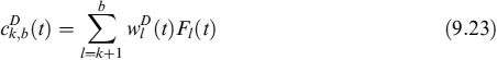
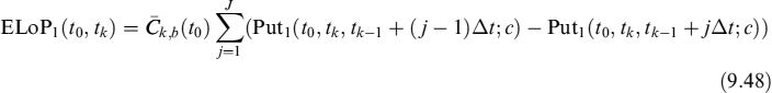
Valuation of the ELoP
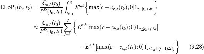
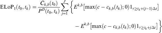
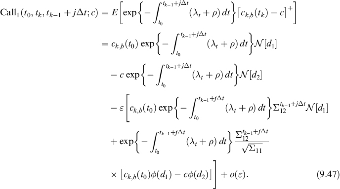
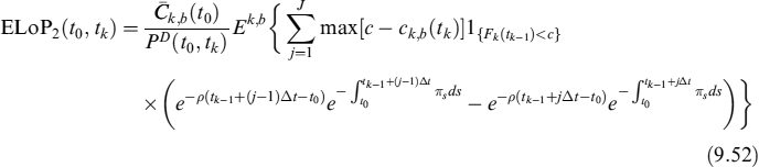
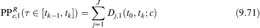
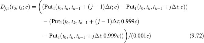
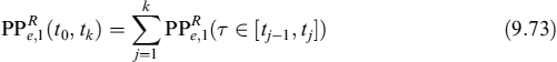
Having derived valuation formulae for the EL, it is straightforward to value the ELoP, for prepayments in {tk}. We indicate this expected loss on prepayment as ELoP1, since we will afterward introduce a second type of rational prepayment. In the most general formulation, it is:
![]()
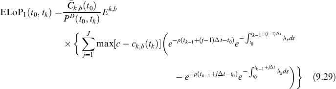
Equation (9.27) is the most general form to value the ELoP1 and includes both the amortizing and non-amortizing cases we have shown above. So we will focus on solving this equation. We move to the forward mortgage rate ck, b(tk) measure, so that:

The first simplification we make is to assume that the prepayment decision (whose effects manifest themselves at the next payment date in any event) occurs at discrete times between [tk−1, tk], which for our purposes are divided into J intervals whose length is ![]() so that we can write (by applying Fubini's lemma as well):
so that we can write (by applying Fubini's lemma as well):
or equivalently
More explicitly we have:
9.2.7 Analytical approximation for ELoP1
Equation (9.29) does not admit an explicit analytical solution, but an analytical approximation is viable. We start from a more general case of the pricing of an option when the instantaneous interest rate is correlated with the underlying asset.16 Let us focus first on valuing a payoff of the kind:
where St is an exponential martingale:
with solution S(t0) = S0 equal to:
where σt is a deterministic function of t. Assume also that the stochastic interest rate ![]() is described by the dynamics:
is described by the dynamics:
with 0 ≤ ε ≤ 1. We assume that dW1t and dW2t are correlated with the correlation parameter ![]() .
.
When the instantaneous interest rate follows CIR dynamics, we have that ![]() is
is
with expected value at time t:
We then get
and the underlying asset's dynamics is
Under this specification, it can be shown17 that:
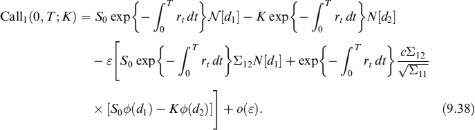
which can be seen as a standard BS formula plus a correction factor due to the correlation between the interest rate and the underlying asset. Terms Σ11 and Σ12 are:
where
and
Now, if we set St = ck,b(t) and we consider the interest rate as the stochastic prepayment intensity λt and include the exogenous rate ρ as well, we can rewrite (9.38):
where the remaining notation is the same as above.
In order to value (9.29), we first need to compute the expected loss over the entire interval [tk−1, tk]. To that end we consider the loss to be given by the terminal payoff, in terms of a put option and not a call. In this case the intensity process λt is correlated only up to each tk−1 + jΔt, and not over the entire interval. So we have to modify ![]() as follows:
as follows:
and
The call option price is then:
Basically, it provides the value of a call option subject to survival of the underlying process ck,b(t0) up to tk.
We also need to derive the put value via put–call parity:

where EF1 is the expected value ck,b(t0) in case a prepayment does not occur before tk. It can be computed as a call option struck at 0: EF1(t0, T, tk) = Call1(t0, T, tk; 0). The prepayment probability PP is calculated as in equation (9.6).
We now have all we need to compute (9.29), which can be rewritten as follows:
9.2.8 Valuing the ELoP using a VaR approach
Intensity λ cannot easily be hedged using market instruments, since no standard contract exists whose value depends on rational prepayment intensity. A possible conservative approach to valuation of the ELoP would be to consider an intensity process occurring at a high level with a given confidence level (say, 99%).
For our purposes, we need to use this distribution to determine the minimum survival probability from t0 up to each date {tk}, or equivalently the maximum prepayment probability up to {tk}. But what we actually need is the forward risk-adjusted distribution for λt, which is given in equation (8.36).
Assume we want to build an expected survival probability curve up to expiry of the mortgage in tN = T. Assume also that we divide the interval [t0, tN] into N subintervals Δt = [tN − t0]/N. We follow Procedure 9.2.1 which is given in pseudocode.
Procedure 9.2.1. This procedure derives the maximum expected levels of prepayment intensity ![]() , at discrete prepayment dates, with a confidence level (c.l.), say, of 99%:
, at discrete prepayment dates, with a confidence level (c.l.), say, of 99%:
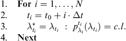
Having determined the maximum default intensity levels, we can compute the term structure of (minimum) survival probabilities SPR(0, ti):
Having determined the minimum rational survival probability, the maximum (total) prepayment probability up to given time {ti} is straightforward:
for i = 1; …, N.
To evaluate the ELoP using a VaR-style approach we need to compute the conditional mean (drift) and conditional volatility of the mortgage rate process as well:18 we know that it is assumed to be lognormally distributed with the mean equal to its forward level (so that the drift of the process of ci, b is zero) and with the volatility parameter the same as in (9.22). Conditional volatility for a mortgage rate at time T, and for a rational intensity process observed in ti ≤ T, is:
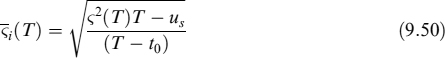
where
![]()
The drift of the process is:
with initial condition ![]() and
and
![]()
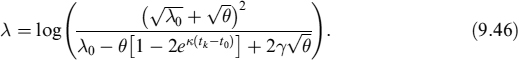
The ELoP can thus be computed with formula (9.48) by using the adjusted forward mortgage rate
![]()
and volatility parameter ![]() .
.
Example 9.2.2. Assume 1Y (risk-free) OIS forward rates with volatilities like those in Table 9.10. Assume further that exogenous prepayment intensity is 3% p.a. and rational prepayment intensity has the same dynamics parameters as presented above. We consider a 10Y mortgage, with a fixed rate paid annually of 3.95%. The fair rate has been computed without taking into account any prepayment effect (credit risk is not considered, although it can be included within the framework). The amortization schedule is in Table 9.11.
Given the market and contract data above, we can derive the EL at each possible prepayment date, which we assume occurs annually. It is plotted in Figure 9.3. A closed-form approximation has been employed to compute the EL. In a similar way it is possible to calculate the ELoP. We also use in this case an analytical approximation that allows for correlation between interest rates and rational prepayment intensity.
In Figure 9.4 the ELoP is plotted for a zero correlation case and for a negative correlation set at −0.8. This value implies that, when interest rates decline, the default intensity increases. Since the loss for the bank is bigger when rates are low, the ELoP in this case is higher than in the uncorrelated case.
Table 9.10. Volatilities of 1Y OIS forward rates
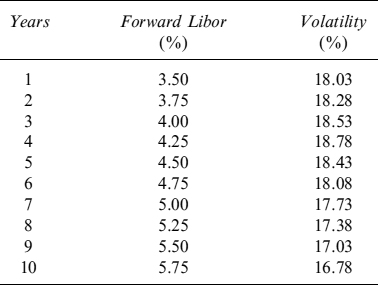
Table 9.11. Amortization schedule of a 10Y mortgage
| Years | Notional |
| 1 | 100.00 |
| 2 | 90.00 |
| 3 | 80.00 |
| 4 | 70.00 |
| 5 | 60.00 |
| 6 | 50.00 |
| 7 | 40.00 |
| 8 | 30.00 |
| 9 | 20.00 |
| 10 | 10.00 |
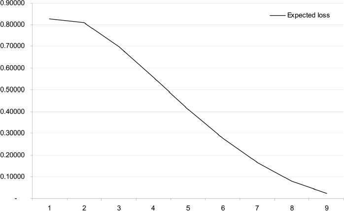
Figure 9.3. Expected loss for a 10-year mortgage
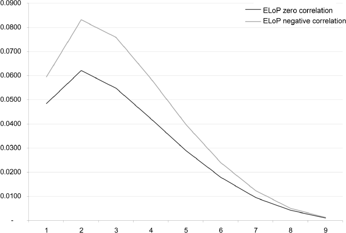
Figure 9.4. Expected loss on prepayment for a 10-year mortgage
9.2.9 Extension to double rational prepayment
The framework designed so far implicitly assumes that rational prepayment is driven by the convenience of closing a live fixed rate mortgage and opening a new one with a corresponding residual maturity and a lower contract rate. An alternative the mortgagor could pursue is to open a new mortgage with a floating rate: although from a theoretical financial perspective the two alternative choices are equivalent, from a behavioural perspective as a result of poor financial skills a comparison between the floating rate (e.g., the 3-month Libor) and the original fixed rate can produce a “rational” reason to prepay.
To model this behaviour, assume that the prepayment decision modelled before resembles a jump whose occurrence is described by an intensity rate π. The decision can be taken at any time, but it produces effects only when the Libor rate is lower than the contract rate Lt < c. The EL is the same as that subsequent to a rational prepayment, whereas the ELoP, which we indicate by ELoP2 in this case, can be written as:
where we have kept the effects of the exogenous prepayment that is operating in any case in mind.
The dynamics of rational intensity π, which only manifests its effects when the Libor rate Fk+1(tk) < c, are specified as follows:
![]()
According to this intensity, the probability that no rational decision is taken up to time T, evaluated at time t, is:
where A(t, T) and B(t, T) are the same as in equation (8.27). ψπ is the market premium for prepayment risk which is also assumedin this case to be 0. We indicate the survival probability in this case as:
and the total prepayment probability is:
To value (9.52) we first need to compute the following:19
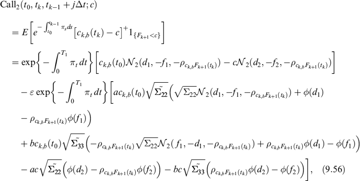
where N2(.;.;.) is the bivariate normal distribution, and:
and
Furthermore

The other two covariances are more difficult to solve explicitly, but we can find an analytical expression for both of them in any case. We define
and
Hence the two covariances can be expressed as
and

We denote by ρck,bπ the correlation between the mortgage rate at time tk and the intensity π, by ρFk+1(tk)π the correlation between the Libor rate fixing at time tk and the intensity π and, finally, by ρck,bFk+1(tk) the correlation between the mortgage rate and Libor at time tk. The last quantity can be derived by means of the formula:
where the notation is the same as that used above. We use the well-known procedure of freezing Libor rates at the level prevailing at time t0.
We can derive the put via put–call parity:

The quantity EL2(t0, tk, tk−1 + jΔt; c) is equal to ![]() and can be computed as the price of Call2(t0, tk, tk−1 + jΔt; 0), forcing the following quantities in formula (9.56) (although the strike c = 0) to be:
and can be computed as the price of Call2(t0, tk, tk−1 + jΔt; 0), forcing the following quantities in formula (9.56) (although the strike c = 0) to be:
and
Finally, we are able to compute the expected loss on prepayment

Total ELoP of this extended version of the model is the sum of ELoP1 in (9.48) and ELoP2 in (9.68) (ELoP = ELoP1 + ELoP2). This will also be the ELoP used to compute total prepayment cost, that we define in the following section.
9.2.10 Total prepayment cost
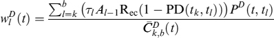
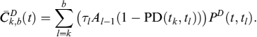
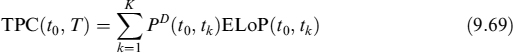
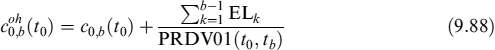
The ELoP is a tool to measure expected losses a bank will suffer upon prepayment. For hedging and pricing purposes, though, it is more useful to compute total prepayment cost (TPC), defined as the sum of the present values of ELoP(t0, tk) for all possible K prepayment dates in the interval [t0, tb = T]:
TPC can be hedged, since it is a function of Libor forward rates and related volatilities entering in the mortgage rate ck,b(t0): TPC(t0, T)→TPC(t0, T; F(t1), …, F(tb−1), σ1,…, σb−1). As for its sensitivity to interest rates, we can bump a given amount (say, 10 bps) separately each forward and then calculate the change in TPC. Denoting by ΔδF(ti) TPC the sensitivity of TPC with respect to bump δF(ti) of the forward F(ti), we have that:

In an analogous fashion we can compute its sensitivity to volatilities:

These sensitivities can easily be converted in hedging quantities of liquid market instruments, such as swaps and caps and floors.
9.2.11 Expected cash flows
The model can also be employed to project expected cash flows, taking into account the prepayment effect. More specifically, as already stated, the rational prepayment decision may occur at any time, but the actual effects both in terms of anticipated unwinding of the contract and of costs for the bank, manifest themselves only when the condition that the forward mortgage rate is lower than the contract rate ck,b(tk) < c is verified. In the previous section we considered this condition, since we only calculate the P&L effects when ck,b(tk) < c. Actually, the bank always suffers a loss in this case.
When projecting expected cash flows, the probability of an anticipated inflow of the residual notional at a given time tk has to be computed as follows:
where ![]() is the survival probability jointly with condition ck, b(tk) < c, which we name “effective”. The latter can be calculated by exploiting the approach described above for the ELoP: so we start with the effective rational prepayment probability in the interval [tk−1, tk]. Assume we divide this into J subintervals Δt
is the survival probability jointly with condition ck, b(tk) < c, which we name “effective”. The latter can be calculated by exploiting the approach described above for the ELoP: so we start with the effective rational prepayment probability in the interval [tk−1, tk]. Assume we divide this into J subintervals Δt
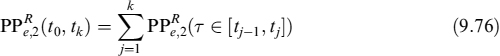
The notation and pricing formulae for the put options are the same as above. In practice, we calculate the price of a digital option in case it terminates before expiry with a probability determined by rational prepayment intensity λt. The effective prepayment probability from t0 up to a given time tk can be obtained by summing all the probabilities relating to prepayment times occurring before tk and including the latter as well:
This quantity is used in (9.70) since ![]() .
.
The same can also be done if a second type of rational prepayment is introduced, so that:
where

and
Total survival probability if we keep this additional rational prepayment in mind would be ![]() .
.
Expected total cash flow (interest + capital) at time t0 for each scheduled payment time20 {tj = tk} is given by the formula:
The expected outstanding amount at each time is given by:
It will be useful to define the prepayment-risky annuity, PRDV01:

and the present value of the sum of expected capital cash flows PVECF:
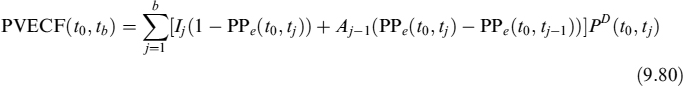
Both quantities can be computed with respect to standard prepayment probabilities or those derived by means of a VaR approach. Moreover, both can be compared with equivalent quantities when no prepayment risk is considered. Hence we have the DV01:
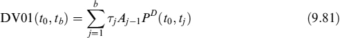
and the present value of the sum of the contract capital cash flows CF:
9.2.12 Mortgage pricing including prepayment costs
The fair rate of a mortgage at inception has to take into account two effects of prepayment. The first effect is due to the fact that prepayment is equivalent to accelerated amortization, so that the bank receives earlier than expected the amount lent to the mortgagee: this produces a lowering of the fair mortgage rate. This effect is gauged by weighting future cash flows with prepayment probabilities. The second effect is due to the cost that the bank bears when prepayment occurs when the replacement of the mortgage in the bank's assets can be operated at a rate lower than the original one: we have measured this cost using the TPC.
Let us start with the fair rate at time t0 of a mortgage with notional A starting at t0, ending at T = tb, with a predefined amortization schedule:
This formula does not include any effect due to prepayment. We can include the first effect mentioned above by replacing the DV01 and the present value of the contract's capital cash flows by their expected value:
where the superscript pw stands for prepayment weighted. The effect of anticipating the amortization implies that ![]() . To calculate a full risk fair rate that also includes the cost stemming from prepayment, formula (9.84) modifies as follows:
. To calculate a full risk fair rate that also includes the cost stemming from prepayment, formula (9.84) modifies as follows:
Equation (9.85) acknowledges to the mortgagee both the benefits and costs for the bank in case of prepayment. A more conservative approach would be to include the TPC computed with a VaR approach, instead of the standard approach. An alternative would be to charge the TPC, split over the expected life of the contract, over the fair rate with no prepayment risk:
This rate can be considered the standard fair rate including prepayment cost but not the first prepayment effect (accelerated amortization).
Finally, to give an idea of the maximum rate that can be charged to the mortgagee, we consider overhedging the TPC, which is simply the summation of all the expected losses EL without any weighting for the prepayment probability. In this case the formula for the mortgage rate is:

as long as we are only considering the first prepayment effect. Otherwise, we simply add total expected loss (split over the expected life of the contract) to the standard fair rate:
Example 9.2.3. Considering the case in Example 9.2.2, we now compute the TPC related to the 10-year mortgage, which is equal to 48 bps.
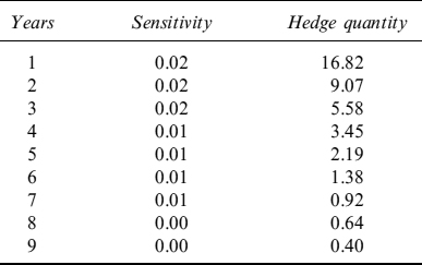
Table 9.12 shows the sensitivity of the TPC to a tilt of 10 bps for each forward rate. These sensitivities are then translated in an equivalent quantity of swaps, with expiries from 1 year to 10 years, needed to hedge them.
Table 9.13 shows the Vega of the TPC with respect to the volati'/ities of each forward rate. These exposures can hedged using caps and floors or swaptions in the Libor market model setting we are working in (by calibrating the forward rate correlation matrix to the swaption volatility surface).
Table 9.12. Interest rate sensitivity of the TPC
| Years | Vega |
| 1 | 0.08 |
| 2 | 0.20 |
| 3 | 0.33 |
| 4 | 0.45 |
| 5 | 0.53 |
| 6 | 0.54 |
| 7 | 0.48 |
| 8 | 0.33 |
| 9 | 0.12 |
Let us now assume we want to include the prepayment cost in the 10-year mortgage. We first include exogenous prepayment, which is independent of the level of interest rates, so that on average its effects boil down to anticipated repayment of the outstanding notional: this will reduce the fair rate and, according to the data we used above, we have the fair rate modified as:
c = 3.95% → c = 3.89%
Second, we include the TPC arising from rational prepayment (48bps), which surely entails an increase of the fair rate:
c = 3.89% → c = 4.00%
or the total effect of the prepayment of 5 bps in the fair rate.
For comparison purposes, we consider the overhedge strategy which consists in replication of the EL instead of the ELoP. In this case the fair mortgage rate would change as follows:
c = 3.89% → c = 4.78%
As mentioned in the main text, while the interest rate and volatility risk can be hedged using standard (and liquid) market instruments, the prepayment risk related to the stochasticity of (rational prepayment) intensity cannot be eliminated. We suggest a VaR-like approach to resolve this. The corresponding TPC for the 10-year mortgage is 56 bps and the fair rate modifies as:
c = 3.89% → c = 4.02%
which means that a generally higher prepayment probability has little impact on pricing. In Table 9.14 we show a comparison between expected and 99th percentile rational prepayment probabilities. Higher probability increases the costs but, since it also anticipates prepayment, the likelihood to have larger differences between current and mortgage rates is reduced.
Table 9.14. Expected and 99th percentile prepayment probabilities from the first to the last possible prepayment date
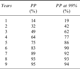
Table 9.15. Sets of parameters, fair rates and TPC (using standard and VaR-like approaches)
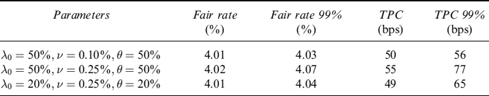
To appreciate the effect of different parameters on the TPC, in Table 9.15 we show three sets of parameters of the intensity dynamics of rational prepayment and their effect on:
- the fair rate;
- the fair rate at 99th percentile prepayment probabilities;
- the TPC;
- the TPC at 99th percentile prepayment probabilities.
The total effect is rather limited for the mortgage fair rate. When considering the TPC, the differences between the base and VaR-like approach are bigger.
Example 9.2.4. We now show how the model presented works for a portfolio of mortgages. The Eonia discount factors and zero rates (in percent), for years 1 to 30, that we have used have been extracted from deposits, FRAs and swaps on Euribor (shown in Table 9.16). In Table 9.17 we show volatilities for the forward rates needed to compute the EL.
We consider a portfolio of 307,048 mortgages worth a total amount of EUR1 billion. The distribution of contract fixed rates within the portfolio is given in Table 9.18 and represented in Figure 9.5.
The distribution of notional amounts is shown in Table 9.19 and Figure 9.6. The vast majority of mortgage notional amounts were less than EUR200,000, and only 506 contracts were above 500,000 euros and 111 above EUR1 million.
Finally, we show the distribution of maturities within the portfolio in Table 9.20 and Figure 9.7. Mortgage maturity is mainly concentrated on 10 years and 20 years; fewer contracts have shorter maturities and only 1.31% of the total portfolio has an expiry after 30 years.
Table 9.16. Eonia discocunt factors and zero rates for maturities from 1 to 30 years
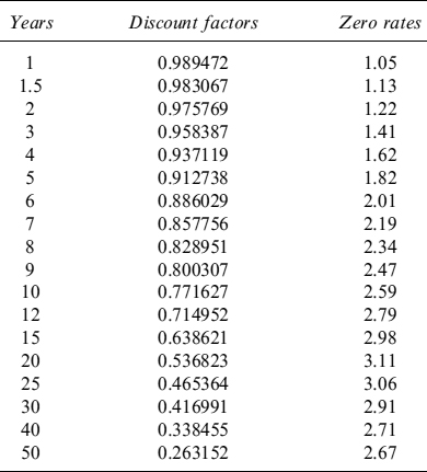
Table 9.17. Volatilities of Eonia forward rates for maturities from 1 to 30 years
| Years | Volatility |
| 1 | 44.41 |
| 1.5 | 51.01 |
| 2 | 53.38 |
| 3 | 47.99 |
| 4 | 45.87 |
| 5 | 42.64 |
| 6 | 39.27 |
| 7 | 36.31 |
| 8 | 33.86 |
| 9 | 31.93 |
| 10 | 30.35 |
| 12 | 27.80 |
| 15 | 25.50 |
| 20 | 23.77 |
| 25 | 23.59 |
| 30 | 24.40 |
Total prepayment cost (TPC), given market conditions at the evaluation date, is around EUR49 million (see Table 9.21). This is a not a small percentage of the outstanding notional amount (remaining capital) of the mortgages. TPC is the current value of expected losses incurred in the future from the prepayment decisions taken by mortgagees.
Table 9.18. Distribution of contract fixed rates for the mortgage portfolio
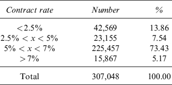
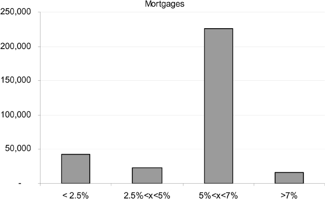
Figure 9.5. Distribution of contract fixed rates for the mortgage portfolio
The possibility to hedge this quantity is crucial to minimize the costs related to prepayments. In a low-margin environment for the bank, such a cost is definitely not negligible. Prepayment exposures must be monitored and appropriate hedging strategies must be implemented.
Zero rate sensitivities are reported in Table 9.22 for different tenors from 1 year to 30 years: most exposures are between 10 years and 25 years. For a parallel shift in the zero rate curve of 1 basis point, variation in TPC is of about EUR145,000. The bank gains (i.e., TPC decreases) when rates move up.
Exposures to volatilities are shown for expiries running from 1 to 30 years in Table 9.23. Most sensitivity is on expiries between 10 and 20 years. An upward shift of the term structure of market implied volatilities produces an increase in TPC of about EUR420,000.
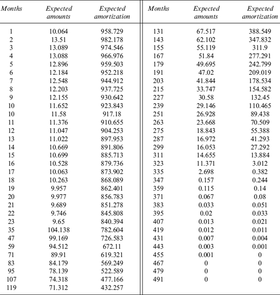
The expected cash flows and amortization of the pool of mortgages for each month, running from the calculation date to 41 years, are shown in Table 9.24. Expected cash flows include contract repayments (capital and interest) weighted by the probability of no prepayment and the full reimbursement of the remaining capital, plus interest for the last period, weighted by the probability of prepayment. Expected amortization includes the amount of capital to be repaid weighted by the no prepayment probability and the amount of remaining capital paid back when the mortgage ends before expiry, wighted by the prepayment probability.
Table 9.19. Distribution of notional amounts for the mortgage portfolio
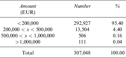
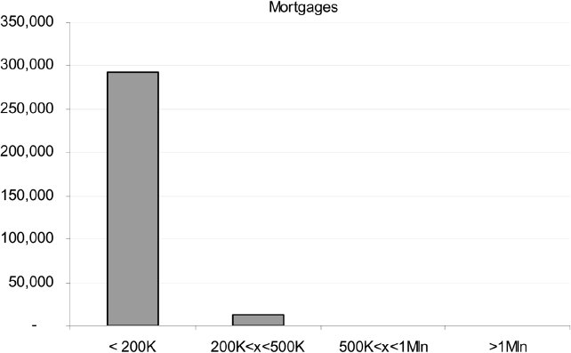
Figure 9.6. Distribution of notional amounts for the mortgage portfolio
Table 9.20. Distribution of maturities for the mortgage portfolio
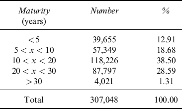
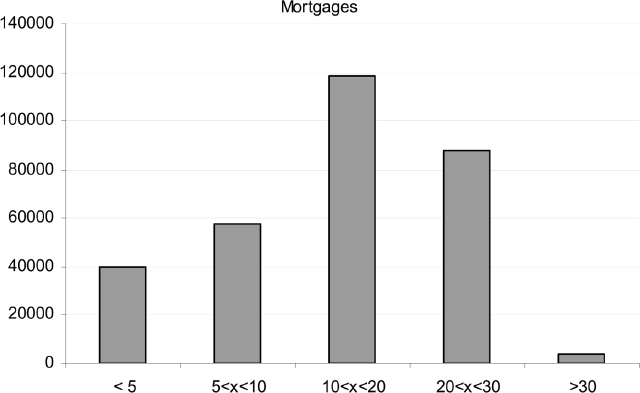
Figure 9.7. Distribution of maturities for the mortgage portfolio
Table 9.21. Total prepayment cost of the portfolio of mortgages
| total | percent |
| 48,736,032 | 4.874 |
Table 9.22. Zero rate sensitivities of the TPC of the portfolio of mortgages
| Years | Zero rate sensitivity |
| 1 | −2,203.03 |
| 2 | − 1,462.35 |
| 3 | −2,336.41 |
| 4 | − 1,652.77 |
| 5 | − 1,068.93 |
| 6 | −575.21 |
| 7 | 2,289.25 |
| 8 | 5,928.28 |
| 9 | 7,129.96 |
| 10 | 9,665.28 |
| 12 | 16,813.30 |
| 15 | 33,398.23 |
| 20 | 46,136.98 |
| 25 | 31,621.84 |
| 30 | 3,291.74 |
| Total | 146,976.18 |
Table 9.23. Volatility sensitivities of the TPC of the portfolio of mortgages
| Years | Vega |
| 1 | −361.1 |
| 1.5 | −705.2 |
| 2 | −2,375.5 |
| 3 | − 10,554.2 |
| 5 | −31,045.8 |
| 7 | −51,706.8 |
| 10 | − 119,649.7 |
| 15 | −121,675.8 |
| 20 | −67,321.9 |
| 30 | −13,647.9 |
| Total | −419,043.9 |
9.3 SIGHT DEPOSIT AND NON-MATURING LIABILITY MODELLING
The modelling of deposits and non-maturing liabilities is a crucial task for liquidity management of a financial institution.21 It has become even more crucial in the current environment after the liquidity crisis that affected the money market in 2008/2009.
Typically, the ALM departments of banks involved in the management of interest rate and liquidity risks face the task of forecasting deposit volumes, so as to design and implement consequent liquidity strategies.
Moreover, deposit accounts represent the main source of funding for the bank, primarily for those institutions focused on retail business, and they heavily contribute to the funding available in every period for lending activity (see Chapter 7). Of the different funding sources, deposits have the lowest costs, so that in a funding mix they contribute to reducing the total cost of funding.22
Indeed, deposit contracts have the peculiar feature of not having a predetermined maturity, since the holder is free to withdraw the whole amount at any time. The liquidity risk for the bank arises from the mismatch between the term structures of assets and liabilities of the bank's balance sheet, since liabilities are mostly made up of non-maturing items and assets by long-term investments (such as mortgage loans). We extensively analysed this problem in Chapter 7.
The optionality embedded in non-maturing products, relating to the possibility for the customer to arbitrarily choose any desired schedule of principal cash flows, has to be understood and accounted for when performing liability valuation and hedging market and liquidity risk. Thus, a sound model is essential to deal with embedded optionality for liquidity risk management purposes.
Table 9.24. Expected cash flows and amortization schedule of the portfolio of mortgages
9.3.1 Modelling approaches
Two different approaches can be found in the financial literature and in market practice to model the evolution of deposit balances:
- bond portfolio replication
- OAS models.
Bond portfolio replication, probably the most common approach adopted by banks, can be briefly described as follows. First, the total deposit amount is split into two components:
- a core part that is assumed to be insensitive to market variable evolution, such as interest rates and deposit rates. This fraction of the total volume of deposits is supposed to decline gradually over a medium to long-term period (say, 10 or 15 years) and to amortize completely at the end of it.
- a volatile part that is assumed to be withdrawn by depositors over a short horizon. This fraction basically refers to the component of the total volume of deposits that is normally used by depositors to match their liquidity needs.
Second, the core part is hedged using a portfolio of vanilla bonds and money market instruments, whose weights are computed by solving an optimization problem that could be set according to different rules. Typically, portfolio weights are chosen so as to replicate the amortization schedule of deposits or, in other words, their duration. In this way the replication portfolio protects the economic value of the deposits (as defined later on) against market interest rate movements. Another constraint, usually imposed in the choice of portfolio weights, is target return expressed as a certain margin over market rates.
Since deposit rates are updated, with relatively large freedom of action, by banks to align them with market rates, the replication portfolio can comprise fixed rate bonds, to match the inelastic part of deposit rates that do not react to changes in market rates, and floating rate bonds, to match the elastic part of deposit rates. The process to rebalance the bond portfolio, although simple in theory, is quite convoluted in practice. For a more detailed explanation of the mechanism see [86].
Third, the volatile part is invested in very short term assets, typically overnight deposits, and represents a liquidity buffer to cope with daily withdrawals by depositors.
The critical point of this approach is estimation of the amortization schedule of non-maturing accounts, which is performed on a statistical basis and has to be reconsidered periodically. One of the flaws of the bond replica approach is that risk factors affecting the evolution of deposits are not modelled as stochastic variables. So, once statistical analysis is performed, the weights are applied by considering the current market value of the relevant factors (basically, market and deposit rates) without considering their future evolution.
This flaw is removed, at least partially, by the so-called option-adjusted spread (OAS) approach, which we prefer to call the stochastic factor (SF) approach.23 In principle, the approach is little different from the bond portfolio replica approach: it identifies statistically how the evolution of deposit volumes is linked to risk factors (typically, market and interest rates) and then sets up a hedge portfolio that covers their exposures.
The main difference lies in that, in contrast to bond portfolio replication, in the SF approach the weights of hedging instruments are computed keeping the future random evolution of risk factors in mind, so that the hedging activity resembles the dynamic replication of derivatives contract. The hedging portfolio is revised based on the market movements of risk factors, according to the stochastic process adopted to model them.
We prefer to work with a SF approach to model deposit volumes for several reasons. First, we think the SF approach is more advanced from the modelling perspective, explicitly taking into account the stochastic nature of risk factors. Second, if bond portfolio replication can be deemed adequate to hedge the interest rate margin and the economic value of deposits, from the liquidity risk management point of view the SF approach is superior, by the very fact that it is possible to jointly evaluate within a unified consistent framework the effects of risk factors both on the economic value and on future inflows and outflows of deposits. Third, it is easier to include complex behavioural functions linking the evolution of volumes to risk factors in the SF approach. Finally, bank-run events can also be considered and properly taken into account in the SF approach, whereas their inclusion seems quite difficult within the bond portfolio replication approach.
9.3.2 The stochastic factor approach
The first attempt to apply the SF approach, within an arbitrage-free derivatives-pricing framework, to deposit accounts was made by Jarrow and van Deventer [78]. They derived a valuation framework for deposits based on the analogy between these liabilities and an exotic swap whose principal depends on the past history of market rates. They provide a linear specification for the evolution of deposit volumes applied to US federal data.
Other similar models have been proposed24 within the SF approach: it is possible to identify three building blocks common to all of them:
- A stochastic process for interest rates: in [78], for example, it is the Vasicek model (see Chapter 8).
- A stochastic model for deposit rates: typically, these are linked to interest rates by means of a more or less complex function.
- A model for the evolution of deposit volumes: since this is linked by some functional forms to the two risk factors in points 1 and 2, it too is a stochastic process.
Specification of the dynamics of deposit volumes is the crucial feature distinguishing the different SF models: looking at things from the microeconomic perspective, volumes depend on the liquidity preference and risk aversion of depositors, whose behaviour is driven by opportunity costs between alternative allocations. When market rates rise, depositors have a greater temptation to withdraw money from sight deposits and invest them in other assets offered in the market.
SF models can be defined behavioural in the sense that they try to capture the dynamics of depositor behaviour with respect to market rates and deposit rates movements. In doing this, these models exploit option-pricing technology, developed since the 1970s, and depend on stochastic variables, in contrast to the previously mentioned class on simpler statistical models.
Depositor behaviour can be synthesized in a behavioural function that depends on risk factors and determines their choice in terms of the amount allocated in deposits. This function could be specified in various forms, allowing for different degrees of complexity. Given their stochastic nature, those models are suitable for implementation in simulation-based frameworks like Monte Carlo methods.
Since closed-form formulae for the value of deposits are expressed as risk-neutral expectations, the scenario generation process has to be accomplished with respect to the equivalent martingale probability measure. For liquidity management purposes, it is more appropriate to use real-world parameter processes. In what follows we will not distinguish between them: as we have also assumed in other parts of this book, with a risk premium parameter equal to zero, real-world processes for interest rates clash with risk-neutral ones.
We propose a specification for the SF approach which we think is parsimonious enough, yet effective.
Modelling of market interest rates
The dynamics of market interest rates can be chosen rather arbitrarily: the class of short-rate models we introduced in Chapter 8 is suitable and can be effectively used. In our specification we adopted a single-factor CIR++ model (see Section 8.3.4): we know that such a model is capable of perfectly matching the current observed term structure of risk-free zero rates. The market instantaneous risk-free rate is thus given by
rt = xt + ϕt
where xt has dynamics
![]()
and ϕt is a deterministic function of time.
Modelling of deposit rates
Deposit rate evolution is linked to the pricing policy of banks, providing a tool that can be exploited to drive deposit volumes across time. It is reasonable to think that an increase in the deposit rate will work as an incentive for existing depositors not to withdraw from their accounts or to even increase the amount deposited.
The rate paid by the bank on deposit accounts can be determined according to different rules. Here are some examples:
- Constant spread below market rates:
to avoid having negative rates on the deposit, there is a floor at zero.
- A proportion α of market rates:
We analysed the fair pricing of sight deposits and non-maturing liabilities in Chapter 7, where we also derived the fair rate that a bank should pay on these contracts, discovering that it is a functional form of the kind in equation (9.90).
- A function similar to the two above but also dependent on the amount deposited:
where Dj and Dj+1 are the range of deposit volumes D producing different levels of deposit rates.
We adopt a rule slightly more general than equation (9.90) (i.e., a linear affine relation between the deposit rate and the market short rate):
where E(ut) = 0, ∀t.
As will be manifest in what follows, the evolution of deposit volumes depends on the deposit rate, so in this framework the pricing policy function, which is obviously discretionary for the bank, represents a tool to drive deposit volumes and, consequently, can be used to define liquidity strategies.
Modelling of deposit volumes: linear behavioural functions
We can model the evolution of total deposit volumes by establishing a linear relationship between its log variations and risk factors (i.e., market interest and deposit rates): this is the simplest behavioural functional form we can devise. Moreover, we add an autoregressive component, by imposing the condition that log variation of the volume at a given time is linked to log variation of the previous period with a given factor and, finally, we also include a relationship with time, so as to detect time trends. Volume evolution in this case is given by the equation:
with Δ being the first-order difference operator and ![]() the idiosyncratic error term with zero mean. This formula is in practice the same as the one given in [78].
the idiosyncratic error term with zero mean. This formula is in practice the same as the one given in [78].
Model (9.93) is convenient because the parameters can easily be estimated on historical data via the standard OLS algorithm.
The presence of a time component in equation (9.93) is justified by empirical evidence on deposit series, which exhibits a trend component. This factor could be modelled in alternative ways, substituting the linear trend with a quadratic or exponential one.
For interest rate risk management purposes, it is interesting to understand how deposit evolution can be explained only by market and deposit rate movements. To this end, we introduce a reduced version of the model that can be estimated minus the trend component; that is:
Empirical analysis of both model forms will be presented below.
Modelling of deposit volumes: nonlinear behavioural models
The behavioural function linking the evolution of deposit volume to risk factors can also be nonlinear, possibly involving complex forms. In recent years some efforts have been made to formulate this relation according to more sophisticated functions that describe peculiar features of deposit dynamics. The main contribution in this direction was provided by Nystrom [97], who introduced a nonlinear dependency of the dynamics of deposit volumes on interest rates in the valuation SF framework we are discussing. Formalization of such dynamical behaviour is not trivial and we propose a model specification, inspired by [97].
The main reason nonlinear behavioural functions have been proposed is equation (9.93) has a drawback: it does not allow empirically observed depositor reactions to market and deposit rate movements to be fully captured. Actual behaviour exhibits high nonlinearity with respect to these, in the sense that it depends not only on variations, as implied by equation (9.93), but also on the levels of market and deposit rates.
The main idea behind modelling nonlinear behaviour is based on the microeconomic liquidity preference theory: depositors (and, generally speaking, investors) prefer to keep their investments liquid when market rates are low. As market rates increase, the preference for liquidity is counterbalanced so that depositors transfer higher fractions of their income and wealth to less liquid investments.
Looking at this in greater detail, the first variable to consider is total depositor income I, growing at an annual rate ρ: on an aggregated base we could regard it as the growth rate of the economy (GDP) or simply the growth rate of the income for each depositor (customer).
Second, allocation of the income between deposits and other (less liquid) investments hinges on the following assumptions:
- each depositor modifies his balance in the deposit account by targeting a given fraction
 of his income I. This level can be interpreted as the amount needed to cover his short-time liquidity needs. At any time t, given the current fraction λt of the income invested in deposits, adjustment toward the target occurs at speed ζ;
 - there is an interest rate strike level E, specific to the customer, such that when the market rate is higher he then reconsiders the target level and redirects a higher amount to other investments (i.e., fraction γ of his income);
- there is a deposit rate strike level F, specific to the customer, such that when the rate received on deposits is higher he then is more reluctant to withdraw money (i.e., fraction δ of his income).
Under these assumptions, evolution of fraction λt of the income allocated in sight deposits is:
where 1[E,∞) is the indicator function equal to 1 when the condition in the subscript is verified. Income I grows as follows:
and the deposit volume at time t is:
In reality, since each depositor has different levels of strike rates E and F, due to their preferences for liquidity, on an aggregated basis that considers all the bank's customers there is a distribution of strike rates that reflects their heterogeneity in behaviour. So, when we pass from evolution of single deposits to evolution of the total volume of deposits on a bank's balance sheet, strike rates can be thought to be distributed according to any suitable probability function h(x): in the specification we present here we choose a gamma function; that is:
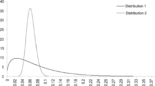
Figure 9.8. Two possible distributions produced by the gamma function (the x-axis shows the interest rate level and the y-axis shows the value of the function h(x)).
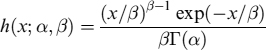
The gamma function is very flexible and allows the distribution to have a wide range of possible shapes.25
Example 9.3.1. As just said, the Gamma function is very flexible and allows for a wide range of possible shapes for the distribution. If we set α = 1.5 and β = 0.05, for example, we have a distribution labelled as “1” in Figure 9.8. If α = 30 and β = 0.002 we have a distribution labelled as “2”. It is possible to model aggregated customer behaviour, making it more or less concentrated around specific levels.
Alternatively, we can use the equivalent functional form of the gamma distribution written as:
![]()
This is actually what we will use to estimate the parameters from historical data shown below.
Evolution of the total volume of deposits can be written by modifying equation (9.95) and considering the distributions of strike rates instead of the single strike rates for each depositor:
where ![]() is the gamma cumulative distribution function.
is the gamma cumulative distribution function.
To make econometric estimation of parameters easier, we rewrite equation (9.98) in the following way:
where ![]() and β= ζΔt.
and β= ζΔt.
Equation (9.99) can be applied by the bank to the “average customer”. Given the heterogeneity of behaviours, given current market and deposit rates, the incentive to change income allocation by increasing less liquid investments, balanced by the incentive to keep the investment in deposits provided by deposit rates, can be synthesized in gamma distribution functions, so that H(x, k, θ) turns out to be the cumulative density of the average customer's strike.
9.3.3 Economic evaluation and risk management of deposits
The three building blocks employed to model deposits can be used to compute the economic value to the bank of the total amount held on the balance sheet.
At time t = 0, for a time horizon T, the economic value is the expected margin that can be earned by the bank on the present and future volume of deposits. In fact, the amount of funds raised by the bank in the form of deposits can be invested in short-expiry risk-free investments yielding rt; on the other hand, the deposit cost to the bank is the rate dt that it has to pay to depositors. Mathematically, this is:

where Dj,t is the amount deposited in account j at time t and n is the number of deposit accounts. Expectation is taken under the equivalent martingale risk-neutral measure Q. Equation (9.100) is the expected net interest margin to the bank over the period [0, T], for all deposit accounts, discounted at 0 by the risk-free discount factor PD.
As suggested in [78], the value of deposits can be regarded as the value of an exotic swap, paying floating rate dj, t and receiving floating rate rt, on the stochastic principal Dj,t for the period between 0 and T.
The approach we outlined above is also a good tool for liquidity risk management, since it can be used to predict expected or stressed ( at a given confidence level) evolution of deposit volumes. To compute these metrics, we need to simulate the two risk factors using a Monte Carlo method (i.e., the risk-free instantaneous interest rate and the deposit rate).26 We undertake the following steps:
- given time horizon T, divide the period [0, T] into M steps;
- simulate N paths for each risk factor;
- compute the expected level of deposit volumes V(0, Ti) at each step i ∈ {0, 1,…, M}, by averaging out N scenarios, by means of equation (9.93) or (9.99):
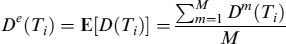
- compute the stressed level of deposit volumes at confidence level p, Vp (0, Ti) at each step i ∈ {0,1,…, M}, based on M scenarios. For liquidity risk management purposes the bank is interested in the minimum levels of deposit volumes at a given time Ti, hence we define the stressed level at the p confidence level as:
Dp(Ti) = inf{D(Ti): P[D(Ti) < Dp(Ti)] ≥ p}
In Chapter 7 we learned how to build the term structure available of funding (TSFu) for non-maturing liabilities. We assumed there that the total amount of deposits dropped by a given percent xNML% in each division of the horizon considered. Actually, the parameter xNML% can also be derived from the model we are using, since it can be inferred by computing the minimum amount of deposit volumes Dp at each time Ti, for i ∈ {1,…, N}, at confidence level p (say, 99%).
Banks may be interested in computing the minimum level of deposits during the entire period between the reference time (say, 0) and a given time Ti: this is actually the value that corresponds to the actual available liquidity that can be used for investments expiring at Ti. To this end it is useful to introduce the process of minima for deposit volumes, defined as:
![]()
Basically, the process excludes all growth in deposit volumes due to new deposits or to an increase in the amount of the existing ones; it only considers the abating effects produced by risk factors. The metric is also consistent with the fact that in any event the bank can never invest more than the existing amount of deposits it has on its balance sheet.
The SF approach can also be used for interest rate management purposes. Once we have the computed the economic value of deposits, it is straightforward to compute their sensitivity to risk factors by setting up hedging strategies using liquid market instruments such as swaps. To this end, we can calculate the sensitivity of the economic value of deposits to perturbations in the market zero-rate curve. Sensitivity to the forward rate F(0; ti, ti+1) = Fi(0) is obtained numerically by means of the following:
where V(·) is provided by (9.100) and ![]() is the relevant forward rate bumped by a given amount (e.g., 10 bps).
is the relevant forward rate bumped by a given amount (e.g., 10 bps).
In Section 9.3.2, we assumed the instantaneous short rate follows single-factor CIR++ dynamics. Let us now assume that the initial zero-rate curve generated by the model (i.e., the series ![]() ) perfectly matches the market-observed term structure, and that we have to modify the short-rate dynamics in a way that produces the desired bump on forward rates at time 0, by suitably modifying the deterministic time-dependent term ϕ(t) of the CIR++ process. This is easily done: let bmp be the size of the bump given to the term structure of the starting forward rate Fi(0); in the CIR++ process the tilted forward
) perfectly matches the market-observed term structure, and that we have to modify the short-rate dynamics in a way that produces the desired bump on forward rates at time 0, by suitably modifying the deterministic time-dependent term ϕ(t) of the CIR++ process. This is easily done: let bmp be the size of the bump given to the term structure of the starting forward rate Fi(0); in the CIR++ process the tilted forward ![]() is obtained by modifying the integrated time-dependent function ϕ(t) as:
is obtained by modifying the integrated time-dependent function ϕ(t) as:
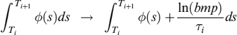
where Ti = Ti+1 − T.
We present below some practical applications of the approach just sketched.
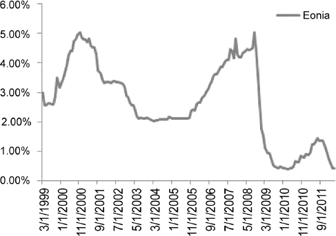
Figure 9.9. Time series of 1-month Eonia swap rates for the period 3/1999:4/2012
Example 9.3.2. We empirically estimate and test the SF approachusing the two behavioural functions presented above, based on public aggregated data for sight deposits in Italy. We considered a sample of monthly observations in the period 3/1999:4/2012 for the total volumes of sight deposits and the average deposit rates paid by the bank. Deposit data are published by the Bank of Italy (see its Bollettino Statistico )27.
We consider the euro 1-month overnight index average (Eonia swap) rate as a proxy for the market short risk-free rate: values for the analysis period are plotted in Figure 9.9.
The CIR model for the market rate was calibrated on a time series of Eonia rates via the Kálmán filter,28 and the resulting values for the parameters were:
κ = 0.053, θ = 7.3, σ = 8.8%
For the second building block (deposit rates), the linear relation between market rates and deposit rates in equation (9.92) was estimated via the standard OLS algorithm (results are shown in Table 9.25). Figure 9.10 plots the actual time series of deposit rates and fitted values from estimated regression. The model shows the time series to be a good fit and we can observe that the linear affine relation is strongly consistent with the data.
Finally, we need to adopt a behavioural function. We start with the linear model for deposit volumes in equation (9.93). The estimation results shown in Table 9.26 prove the model to be a good explanation of the data in this case. We note that the signs of coefficients multiplying, respectively, variations in the market rate and variations in the deposit rate, are opposite as expected. Figure 9.11 plots actual and fitted time series of deposit volumes.
We can now use estimated parameters to compute the economic value of deposits via Monte Carlo simulations of the formula (9.100). The standard approach requires generation of a number of simulated paths for risk factors by means of the estimated dynamics, following these steps:
Table 9.25. Regression results for the deposit rate equation (9.92)
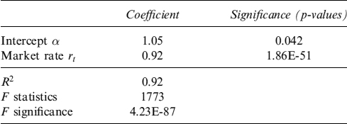
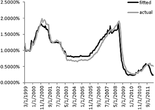
Figure 9.10. Actual time series of deposit rates vs fitted values
Table 9.26. Regression results for the linear behavioural equation (9.93).
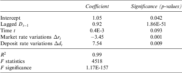
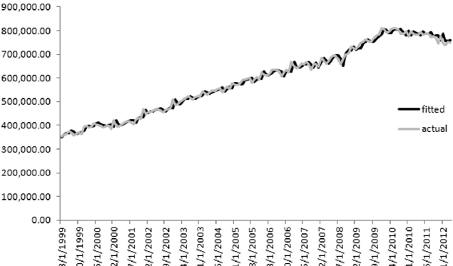
Figure 9.11. Actual time series of deposit volumes vs fitted values for the linear behavioural model
- compute 10,000 paths for market rate evolution, simulated using CIR dynamics;
- for each path, compute the corresponding path for the deposit rate and deposit volumes according to estimated regressions (equations (9.92) and (9.93));
- compute the deposit value at each time step in the simulation period;
- sum discounted values path by path and average them to obtain the present value of the total amount of deposits.
Figure 9.12 shows simulated paths for state variables, using the CIR process with the estimated parameters, starting from the first date after the end of the sample period, the average path of deposit volumes and the minimum amount computed at the 99% c.l. With initial total deposit volumes of EUR834,468 billion and a simulation period of 10 years, the estimated economic value to the bank of holding deposits is EUR121,030 billion.
We also provide empirical results for the reduced version of the linear behavioural model given in equation (9.94). Table 9.27 reports regression parameters for this model, and simulated paths are plotted in Figure 9.13. As expected, excluding the time trend, the forecast for deposit volumes is much more conservative, and the minimum volume at the 99% c.l. rapidly decreases.
We now estimate the parameters of the nonlinear behavioural model in equation (9.99), via a nonlinear least squares algorithm; we still use the same dataset as above (i.e., the sample 3/1999:4/2012 of monthly data for non-maturing deposit volumes, 1-month Eonia swap rates and deposit rates).
In this case, what we actually model is the evolution of proportion λ of depositor income held in sight deposits. At an aggregated level, we approximate the total income to nominal GDP, so that fraction λ will relate to this quantity. Since we are working with Italian deposits, we take Italian GDP data that are published quarterly and undertake linear interpolation to obtain monthly values.29 The reconstructed nominal GDP time series, for the estimation period we consider, is shown in Figure 9.14.
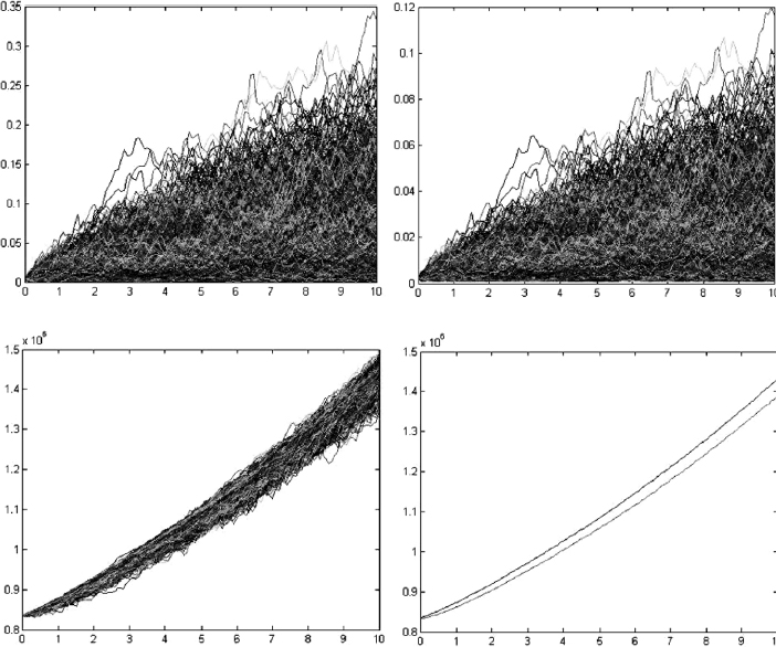
Figure 9.12. (From the top left clockwise) Simulated paths for 1-month Eonia swap rate, deposit rate and deposit volume, term structure of expected future volumes, and minimum (99% c.l.) future volumes
Table 9.27. Regression results for the reduced version of the linear behavioural equation (9.94)
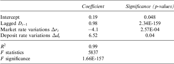
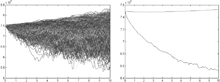
Figure 9.13. (Left) Simulated paths for deposit volumes. (Right) Term structure of expected and minimum (99% c.l.) future volumes
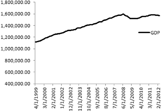
Figure 9.14. Time series of Italian nominal GDP for the sample 3/1999:4/2012. Quarterly data are linearly interpolated to obtain the monthly time series
Estimated coefficients and their significance are shown in Table 9.28. Figure 9.16 plots the probability density function (PDF) of the strike, respectively, for market (E) and deposit (F) rates. We can see that the cumulative density functions are at their highest when the market rate exceeds 3.55% and the deposit rate exceeds 4.25%. These should be considered the levels for market interest rates and deposit rates when most customers are considering reallocating the fraction of income held in deposits in other investments. Regression has an R2 value lower than the linear model tested before: this is also confirmed by the plot of actual vs fitted deposit volumes in Figure 9.15.
Table 9.28. Regression results for the nonlinear behavioural equation (9.99)
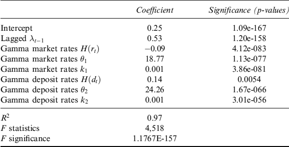
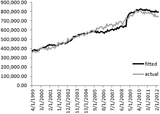
Figure 9.15. Actual time series of deposit volumes vs fitted values for the nonlinear behavioural model
As already done for the linear model, we can compute the economic value of deposits using a Monte Carlo simulation. Figure 9.17 shows simulated paths of deposit volumes and the term structure of expected and minimum volumes. With a simulation period of 10 years and an initial volume of EUR834,467 billion, the economic value of estimated deposits is EUR88,614, so the nonlinear model is more conservative than the linear one.
We can also run Monte Carlo simulations for the nonlinear model after freezing the time trend (which in this case means keeping the GDP constant with the initial level) and the deposit rate. In this way we isolate the effect produced by market interest rates on deposit volumes.
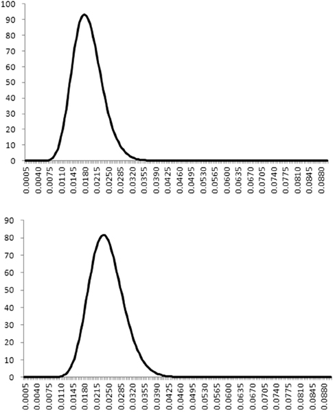
Figure 9.16. Gamma probability density function of the strike level for market interest rates (upper graph) and for deposit rates (lower graph), given the estimated parameters
When just the time trend is frozen we get the results shown in Figure 9.18. It is worthy of note that without the time trend, the fraction of income held in deposits rapidly reaches a minimum and then, given the autoregressive nature of the model in equation (9.99), it keeps constant at this level.
Figure 9.19 shows the results when both the time trend and the deposit rate are frozen: qualitatively, they are the same as when just the time trend is frozen.
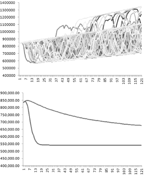
Figure 9.17. Simulated paths (upper graph) and term structure of expected and minimum (99% c.l.) future volumes (lower graph) derived by the estimated nonlinear model
A comparison between the linear and nonlinear model, as far as the expected and minimum level of deposit volumes is concerned, is shown in Figure 9.20. It is quite clear that the nonlinear model seems to be much more conservative in terms of expected and minimum levels of volumes.
We also present a comparison of the market rate sensitivities of the economic value of deposits obtained by the linear and nonlinear model. In Table 9.29 sensitivities to the 1-year forward (risk-free) Eonia rates, fixed every year up to 10 years, are shown. Sensitivities relate to a bump in the relevant forward rate of 10 bps. The linear model has bigger sensitivities due to the higher volumes, and hence higher economic value, expected in the future.
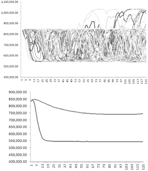
Figure 9.18. Simulated paths (upper graph) and term structure of expected and minimum (99% c.l.) future volumes (lower graph) derived by the estimated nonlinear model when the time trend is frozen
9.3.4 Inclusion of bank runs
It can be interesting to include the possibility of a bank run in the future, due to a lack of confidence by depositors in the creditworthiness and accountability of the bank. If this occurs, it is reasonable to expect a sharp and sudden decline in deposit volumes.
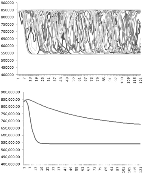
Figure 9.19. Simulated paths (upper graph) and term structure of expected and minimum (99% c.l.) future volumes (lower graph) derived by the estimated nonlinear model when both the time trend and the deposit rate are frozen
To consider a bank run fully, we needs to find some variable that is linked to the bank's credit robustness (or lack of it). The credit spread of the bank on short or long-term debt could be a possible solution: it can either be extracted from market quotes of the bonds issued by the bank or from bank's CDS quotes.
As for the model necessary to simulate this, the very nature of a bank run makes the nonlinear behavioural model more suitable. In fact, it is possible to add an additional behavioural function, related to the bank's credit spread, which will likely be densely concentrated at a high level (denoting an idiosyncratic critical condition). The inclusion of a bank run can be covered by extending formula (9.99) as follows:
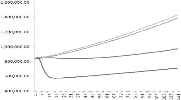
Figure 9.20. Term structure of expected and minimum (99% c.l.) future volumes (lower graph) derived by the linear (equation (9.93)) and the nonlinear (equation (9.99)) model
Table 9.29. Sensitivities to 1Y1Y forward Eonia swap rates of 10 bps up to 10 years for the linear and nonlinear model
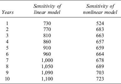
The new behavioural function ![]() is another gamma function taking the bank's spread sB as input.
is another gamma function taking the bank's spread sB as input.
It is quite difficult to estimate the parameters of this function, since it is pretty unlikely the bank has experienced many bank runs. We can resort to bank runs experienced by comparable banks, but even here insufficient events can be observed for robust estimation of the parameters. Nonetheless, the bank can include bank runs on a judgmental basis by assigning given values to the behavioural function according to its hypothesis of stressed scenarios.
Example 9.3.3. We extend the nonlinear model we estimated in Example 9.3.2 to include the possibility of a bank run.
To compute the term structure of expected and minimum deposit volumes we use equation (9.102), using the parameters shown in Table 9.28. The parameters of the additional behavioural function are set as follows:
η = 0.2, k3 = 35, θ3 = 0.002
Given parameters k3 and θ3 of the gamma function, when the credit spread of the bank reaches a level above 800 bps, then a drop of 20% in the level of deposits is experienced in each period (remember, we use monthly steps in our examples).
To model the credit spread and simulate its evolution in the future, we assume that the default intensity of the bank is given by a CIR process as in equation (8.140), with parameters:
λ0 = −0.2, κ = 0.5, θ = 5%, σ = 12%
Moreover, we assume LGD = 60% upon a bank's default. We further assume that the spread entering the behavioural function is the 1-month one for short-term debt.
Figure 9.21 shows the simulated paths and the term structure of expected and minimum deposit volumes: when compared with Figure 9.17 the lower levels projected by the model become evident.
9.4 CREDIT LINE MODELLING
Loan commitments or credit lines are the most popular form of bank lending representing a high percentage of all commercial and industrial loans by domestic banks. Various models exist in the literature for pricing loan commitments: amongst those most recently published are [50], [79] and [12]. These three articles model credit lines by considering as many empirical features as possible, although admittedly many factors enter the valuation and risk management of these types of contracts. In fact, [12] allows for partial usage of credit lines, but the authors do not include in the analysis any dependence between default probability and withdrawals; [50] allows for stochastic interest rates and intensity of default, the probability of using credit lines is linked to default probability, but unfortunately (at least in the specified model) partial and multiple withdrawals are not allowed for; finally, [79] models credit line usage as a function of default probability, with an average deterministic withdrawal that is due to causes other than debtor creditworthiness.
The effects on withdrawals by the default probability and, hence, the spread of the debtor is well documented. This is quite understandable, since when credit lines are committed and no updating clause is included in the contract, the debtor is long an option on its own credit spread struck at the contract spread level specified at inception. This highlights the necessity of using a stochastic model for the probability of default in order to price and monitor financial and liquidity effects appropriately.
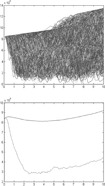
Figure 9.21. Simulated paths (upper graph) and term structure of expected and minimum (99% c.l.) future volumes when bank runs are included
In what follows we present a doubly stochastic intensity-based model for the joint behavior of loan commitments, one that is simple and analytically tractable and incorporates the critical features of loan commitments observed in practice:
- multiple withdrawals by the debtor;
- interaction between the probability of default and level of usage of credit lines;
- impacts on the funding and liquidity buffers to back up the withdrawals.
Furthermore, we design a specific tractable dynamic common factor model for the defaults of several debtors by allowing them to be correlated. Although the Gaussian copula model is an industry standard, it is not easy to adapt this framework to cope with credit lines. We prefer to adopt a reduced-form approach to model defaults. In our analysis, we focus on the doubly stochastic model for default intensity and we assume a common factor affecting the default intensity of all debtor models, thus producing some dependency amongst them. Accordingly, the correlation of withdrawal times and level of withdrawals can be captured by this common component.
We will introduce withdrawal intensity as a function of default intensity. We will achieve two results with such a specification: first, withdrawal intensity increases as default intensity increases, hence accounting for the positive correlation between credit line usage and the level of debtor spread (both of which are functions of default intensity). Second, the joint distribution of the portfolio of credit lines of a financial institution depends on the degree of concentration (or diversification) of the credit risk of debtors. We demonstrate the significant impact resulting from the correlation between default intensity and joint withdrawal distribution.
9.4.1 Measures to monitor usage of credit lines
There are two main measures used in practice to monitor and model credit lines:
- Usage: This is simply defined as the (expected) percentage of the credit line drawn down at any time s (possibly coinciding with the maturity of the credit line) given the observation time t. Mathematically, it can be expressed as:
where DA(s) is the amount drawn at s and CrLn0 is the amount of the credit line opened at inception of the contract at time 0.
- Loan equivalent: This is the percentage of the available amount left, after past withdrawals, which is expected at time t to be used up to time s:
The LEQ metric is commonly used to estimate exposure at default at time T(EAD(T)). It is common practice to assume that usage up to time t is an integral part of exposure at default and the LEQ for the unused portion is added to give total EAD; then, from (9.104), it is quite easy to derive:
EADt(T) = DA(s) + LEQt(T)(CrLn0 − DA(t))
The LEQ has the useful property of allowing the unused portion of a credit line to be modelled separately from the withdrawn portion. It is interesting to note that in empirical studies (see, for example, [115], amongst many others) that both the USG and the LEQ or credit lines lent to defaulted debtors are higher than those lent to surviving debtors.
9.4.2 Modelling withdrawal intensity
The model we present focuses on the usage metric (USG). Consider a bank with a portfolio of m different credit lines, each one with a given expiry Ti (i = 1, 2,…, m). Each credit line can be drawn within limit Li at any time s between today (time t = 0) and its expiry. To model the usage of the line, we introduce withdrawal intensity, which indicates the percentage of the total amount of the line Li drawn down in the infinitesimal interval of time dt.
For credit line i, between today and the maturity Ti, we assume that a debtor can withdraw portions in multiples of 1% of the total amount. Each withdrawal is modelled as a jump from a Poisson distribution Ni(t) with time-varying default intensity ![]() . By construction, it is not possible to consider the effect of more than 100 jumps, since it would represent more than the total amount of the specific credit line, unless we allow for an overdraft. In this case we can set the total number of possible jumps at more than 100. There are several ways to address this problem, but we present two methods: proportional redistribution or cumulated attribution to the last (typically 100th) jump. More details on both methods will be given in Section 9.4.3.
. By construction, it is not possible to consider the effect of more than 100 jumps, since it would represent more than the total amount of the specific credit line, unless we allow for an overdraft. In this case we can set the total number of possible jumps at more than 100. There are several ways to address this problem, but we present two methods: proportional redistribution or cumulated attribution to the last (typically 100th) jump. More details on both methods will be given in Section 9.4.3.
Consider a probability space (Ω, F, Ft, P): since it is not possible to really hedge usage of the line, P represents the physical probability measure. Stochastic withdrawal intensity ![]() for the i-th borrower is a combination of three terms:
for the i-th borrower is a combination of three terms:
where αi is a constant, ρi(t) is a time-dependent deterministic variable and ![]() is default intensity. The specification is rich enough to allow for precise modelling of expected usage at any time t, via functions αi and ρi(t), while the dependence on default intensity
is default intensity. The specification is rich enough to allow for precise modelling of expected usage at any time t, via functions αi and ρi(t), while the dependence on default intensity ![]() introduces a correlation between the worsening creditworthiness of the debtor and higher usage of the credit line.
introduces a correlation between the worsening creditworthiness of the debtor and higher usage of the credit line.
To model the joint usage of m credit lines, it is useful to allow for correlation between the default intensities (and hence default events) of the m debtors as well. We model this by means of an affine correlation: the default intensity of debtor i, for i = 1, 2,…, m, is the sum of two separate intensities:
where ![]() is the i-th debtor's idiosyncratic component, λC(t) is a common factor and pi is a scalar parameter, ranging from 0 to 1, controlling the degree of correlation between debtor default intensities and default events. This model was presented in Chapter 8 and we refer the reader to it for more details. Intuitively,
is the i-th debtor's idiosyncratic component, λC(t) is a common factor and pi is a scalar parameter, ranging from 0 to 1, controlling the degree of correlation between debtor default intensities and default events. This model was presented in Chapter 8 and we refer the reader to it for more details. Intuitively, ![]() is the arrival intensity of default specific to a debtor of line i, while λC is the arrival intensity of a common event which, with some conditional probabilities, causes the default of all debtors in the set of m credit lines, each one with probability pi.30 Given this setting, the borrower may withdraw at any time t ∈ (0, T] with maturity T.
is the arrival intensity of default specific to a debtor of line i, while λC is the arrival intensity of a common event which, with some conditional probabilities, causes the default of all debtors in the set of m credit lines, each one with probability pi.30 Given this setting, the borrower may withdraw at any time t ∈ (0, T] with maturity T.
Equation (9.106) implies that correlation is induced both through a common factor λC in intensities and through a common event. More specifically, conditional on all the independent processes ![]() , there are independent Poisson processes
, there are independent Poisson processes ![]() with these time-varying deterministic intensities. Whenever NC jumps, any borrower i defaults with probability pi, and the default events of the various borrowers, at any such common event time, are conditionally independent. This means there is the potential for more than one borrower to default simultaneously.
with these time-varying deterministic intensities. Whenever NC jumps, any borrower i defaults with probability pi, and the default events of the various borrowers, at any such common event time, are conditionally independent. This means there is the potential for more than one borrower to default simultaneously.
We assume all components of the default process are independent and follow a (pure) Cox–Ingersoll–Ross (CIR) process, which is,
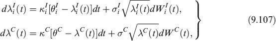
where Wi and Wc are Wiener processes. The drift factor ![]() (respectively, KC[θC − λC (t)]) ensures mean reversion of intensity component
(respectively, KC[θC − λC (t)]) ensures mean reversion of intensity component ![]() towards its long-run value
towards its long-run value ![]() , with the speed of adjustment governed by a strictly positive parameter
, with the speed of adjustment governed by a strictly positive parameter ![]() . The standard deviation factor
. The standard deviation factor ![]() avoids the possibility of there being a negative intensity component
avoids the possibility of there being a negative intensity component ![]() .
.
We set the following parameter constraints:31
- κI = κC = κ
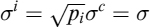 , i = 1, 2, …, m
so that the default intensity ![]() is still a CIR process. In particular,
is still a CIR process. In particular,
where ![]() and the initial value
and the initial value ![]() , i = 1, 2, …, m. In short,
, i = 1, 2, …, m. In short,
where CIR indicates a Cox–Ingersoll–Ross process defined by the arguments within brackets.
Based on equation (9.105), default intensity ![]() is multiplied by a deterministic variable αi. A convenient formula allows the formulae for CIR process parameters to be retained, as seen in Chapter 8, by adjusting the parameters of the process. Equation (9.109) can be rewritten as
is multiplied by a deterministic variable αi. A convenient formula allows the formulae for CIR process parameters to be retained, as seen in Chapter 8, by adjusting the parameters of the process. Equation (9.109) can be rewritten as
Note that the stochastic processes ![]() , λC(t),
, λC(t), ![]() can be considered special cases of basic affine jump diffusions (basic AJD) using a zero-compound Poisson process. The basic AJD model has a closed form that can be used for both the generating function and the characteristic function (for more details see [64]).
can be considered special cases of basic affine jump diffusions (basic AJD) using a zero-compound Poisson process. The basic AJD model has a closed form that can be used for both the generating function and the characteristic function (for more details see [64]).
9.4.3 Liquidity management of credit lines
The framework sketched can be used to derive the usage distribution of a credit line and joint usage of the portfolio of credit lines the bank has. We show how the model is capable of catching the diversification effects produced by the lower or higher correlation between the default probabilities of borrowers. The link between credit risk and usage is also due to default events: these clearly distort the usage distribution, which obviously impacts liquidity management as well.
We will first focus on a single credit line, then we will extend the result to a portfolio of two credit lines: the results can easily be generalized to the case when more lines are involved. We will also see how to derive usage distributions at different times. Finally, the introduction of default events will complete the analysis.
Single credit line
We derive the probability distribution of the usage of one credit line at given time T, given we are at time t. Let us consider a portfolio of a single credit line i and assume for the moment that the time-dependent parameter ρi(t) = 0 for all t. In this case we can combine the two factors for credit risk into one, as as explained above, so that the common component can be neglected. Total withdrawal intensity is then ![]() : we can treat the rescaling parameter αi by making the change of variable in (9.110). The probability that no withdrawal happens (i.e., that no jumps occur) up to time T is given by:
: we can treat the rescaling parameter αi by making the change of variable in (9.110). The probability that no withdrawal happens (i.e., that no jumps occur) up to time T is given by:
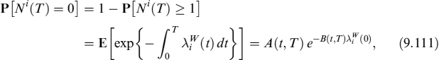
where A(t, T) and B(t, T) have the following forms:
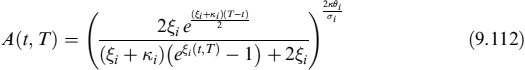
and
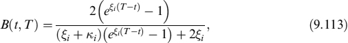
where ![]() .
.
We now need to derive the probability of the number of withdrawals being greater than zero. Based on [64], we numerically know the probability distribution of ![]() . The characteristic function is actually known in closed form.32 The distribution of the integrated factor can therefore be efficiently calculated by Fourier inversion, which is done by carrying out the following steps:
. The characteristic function is actually known in closed form.32 The distribution of the integrated factor can therefore be efficiently calculated by Fourier inversion, which is done by carrying out the following steps:
- Evaluate the characteristic function
 on an unequally spaced grid of length 1,024 whose mesh size is smallest for grid points close to 0 (e.g., by using an equally spaced grid on a logarithmic scale).
 - Fit a complex-valued cubic spline to the output from step 1 and evaluate the cubic spline on an equally spaced grid with 218 points.
- Apply a fast Fourier transform (FFT) to the output from step 2 to obtain the density of
 evaluated on a equally spaced grid.
Figure 9.22 displays the the probability distribution of ![]() .
.
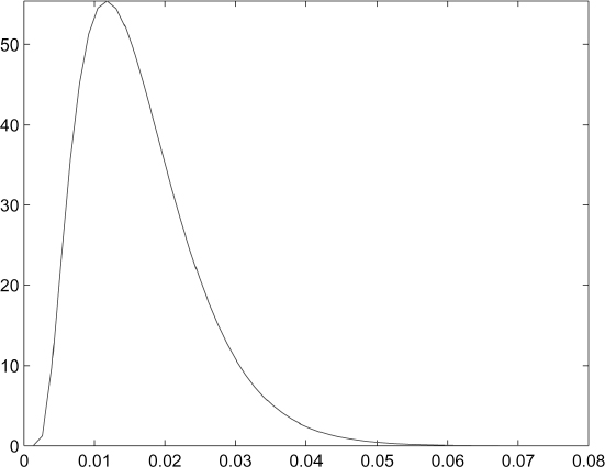
Figure 9.22. The probability distribution of ![]() . Parameters are set at
. Parameters are set at ![]() , σ = 15%,
, σ = 15%, ![]() , αi = 1,
, αi = 1, ![]() and T = 1 year
and T = 1 year
Having numerically evaluated the probability distribution of ![]() , we can evaluate the probability distribution of the Poisson process using the following formula:
, we can evaluate the probability distribution of the Poisson process using the following formula:
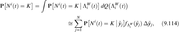
where ![]() ,
, ![]() is the spacing of the grid and N the number of points, i = 1,…, m. The term
is the spacing of the grid and N the number of points, i = 1,…, m. The term ![]() is simply given by the Poisson density function:
is simply given by the Poisson density function:
Adding the time-dependent parameter is also easy, since it means increasing the jump intensity by the quantity ![]() , so that (9.115) becomes:
, so that (9.115) becomes:
Example 9.4.1. We plot the usage (USG) distribution after 1 year of a credit line. As seen above, this is tantamount to computing a Poisson process distribution with jumps from 0 to 100. We assume that the default intensity ![]() is composed of two CIR processes
is composed of two CIR processes ![]() and CIRC(0.015, 0.8, 0.2, 0.015, 1), such that
and CIRC(0.015, 0.8, 0.2, 0.015, 1), such that ![]() . Furthermore, we suppose a coefficient αi = 1,500. Figure 9.23 represents the three plots having a value for the Pi coefficient equal to 0.8: the light-grey line is the plot of
. Furthermore, we suppose a coefficient αi = 1,500. Figure 9.23 represents the three plots having a value for the Pi coefficient equal to 0.8: the light-grey line is the plot of ![]() , the grey line is NC(t) and the dark-grey line Ni(t) is the total distribution, which is defined as total withdrawal intensity. In Figure 9.24 we show the withdrawal distribution when pi = 0.2, with the other parameters as before.
, the grey line is NC(t) and the dark-grey line Ni(t) is the total distribution, which is defined as total withdrawal intensity. In Figure 9.24 we show the withdrawal distribution when pi = 0.2, with the other parameters as before.
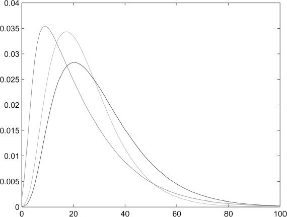
Figure 9.23. In this figure we plot the probability distributions of (i) ![]() in light grey, (ii) NC(t) in grey and (iii) Ni(t) in dark grey. These processes are characterized by the following parameters:
in light grey, (ii) NC(t) in grey and (iii) Ni(t) in dark grey. These processes are characterized by the following parameters: ![]() , CIRC(0.8, 0.2, 0.015, 0.015, 1) and hence
, CIRC(0.8, 0.2, 0.015, 0.015, 1) and hence ![]()
![]() since we have pi = 0.8
since we have pi = 0.8
Percentile evaluation
It is useful to compute the highest withdrawal within the chosen period, at a given confidence level c.l. (e.g., 99%), when pricing and managing the liquidity risk of the credit line. We evaluate the c.l.-percentile of the withdrawal distribution as follows:
- We find the c.l.-percentile of the distribution. We indicate this value by
 ;
; - Using equation (9.116), we evaluate the Poisson distribution of withdrawals using as the new deterministic intensity.
- We calculate the c.l.-percentile of the distribution obtained in the previous step.
Example 9.4.2. Let us consider, for instance, a CIR process characterized by the following parameters: CIR(0.8, 0.15, 0.02, 0.015, 1), which have a multiplying factor equal to αi = 1,500. Let us consider a confidence level of 99%. We find a value for ![]() equal to 62.2217 (as shown in Figure 9.25). This plot is in jump basis, which means that the x-axis goes from 0 to 100 jumps. What we actually need is a different basis: 1% amounts of borrowed money on that specific credit line (as previously specified in Section 9.4.2). If the credit line, for example, has a value of EUR5,000,000, then the largest usage at the 99th percentile is 5,000,000 × 62.2217/100 = EUR3,111,085.
equal to 62.2217 (as shown in Figure 9.25). This plot is in jump basis, which means that the x-axis goes from 0 to 100 jumps. What we actually need is a different basis: 1% amounts of borrowed money on that specific credit line (as previously specified in Section 9.4.2). If the credit line, for example, has a value of EUR5,000,000, then the largest usage at the 99th percentile is 5,000,000 × 62.2217/100 = EUR3,111,085.
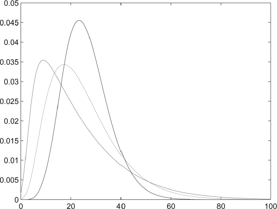
Figure 9.24. In this figure we plot the probability distributions of (i) ![]() in light grey, (ii)ΛC(t) in grey and (iii)
in light grey, (ii)ΛC(t) in grey and (iii) ![]() in dark grey. These processes are characterized by the following parameters:
in dark grey. These processes are characterized by the following parameters: ![]() , CIR(0.8, 0.2, 0.015, 0.015, 1) and hence CIRi(0.8, 0.0894, 0.0230, 0.015, 1) since we have pi = 0.2
, CIR(0.8, 0.2, 0.015, 0.015, 1) and hence CIRi(0.8, 0.0894, 0.0230, 0.015, 1) since we have pi = 0.2
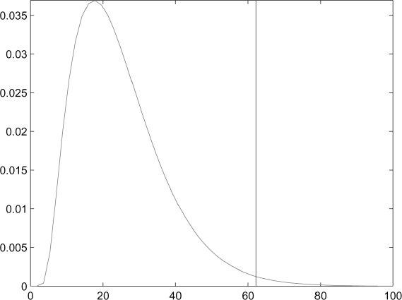
Figure 9.25. The curve represents the density function of integrated stochastic intensity Λi(t) characterized by the following parameters: CIR 0.8, 0.15, 0.02, 0.015, 1. The vertical line represents the 99th percentile of this distribution, which in this case is equal to 62.2217
Dealing with jumps over 100
As already mentioned, if we do not allow an overdraft on the credit line, then we have to deal with jumps above 100 of the Poisson process used to define the withdrawal distribution. Basically, we need to redistribute the probability of jumps above 100 over the full range of jumps between 0 and 100. We here show two methods to cope with this problem: one is the proportional approach, the other is to put all the probability on the last possible jump (i.e., 100).
Looking at this in greater detail, the proportional approach splits the probability of an overdraft on the credit line (i.e., more than 100 jumps) proportionally over the probabilities of the number of jumps from 0 to 100. This redistribution is operated via the formula:
where k = 1,…, 100, ![]() is the cumulated probability of the first 100 jumps and P(R) = 1 − P(L) is the probability of the overdrawn part of the credit line. So, the probability of there being K jumps is adjusted by the fraction of the total probability that has more than 100 jumps, this fraction being proportional to its weight in the cumulated probability of the first 100 jumps. In other words, the method calculates jump probabilities conditioned to having fewer than 100 jumps.
is the cumulated probability of the first 100 jumps and P(R) = 1 − P(L) is the probability of the overdrawn part of the credit line. So, the probability of there being K jumps is adjusted by the fraction of the total probability that has more than 100 jumps, this fraction being proportional to its weight in the cumulated probability of the first 100 jumps. In other words, the method calculates jump probabilities conditioned to having fewer than 100 jumps.
The second approach simply assigns to the 100th jump probability the cumulated probability of there being an overdraft of the line, according to the formula:
where the notation is the same as in the first approach.
Figure 9.26 shows the two redistribution methods we have sketched: (a) represents the proportional approach and (b) shows the last point approach. Of course, expected usage of the credit line is different depending on the method adopted: in fact, expected usage with the proportional method is 28.2877% while it is 29.6318% with the second approach.
Although the first (proportional) approach seems more sensible, the second (last jump) approach allows capturing an effect that has been documented in empirical studies (see, for example, [77]). More specifically, empirical withdrawal distributions seem to be bimodal peaking at around average usage and at full (100%) usage. The second method is best at addressing this situation. However, in what follows we will use only the first method.
Example 9.4.3. We consider usage of a credit line on an amount of L = 5,000,000, using the parameters given in Table 9.30. The probability distribution can be normalized using the procedure described in this section. The results are shown in Figure 9.27. In Table 9.31, we show the values of the 1st and 99th percentiles and the average distribution.
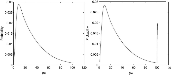
Figure 9.26. (a) Adjusted distribution of jumps (withdrawal percentages of the line) according to the proportional approach. (b) The same distribution adjusted according to the last point approach. Both figures are based on the withdrawal intensity given by a process ![]() and ρ = 0
and ρ = 0
Table 9.30. Parameters used for the single credit line used in Example 9.4.3
| Credit line | |
| L | 5,000,000 |
| κ | 0.8 |
| α | 2,500 |
| λ | 1.735% |
| θ | 1.735% |
| σ | 10.00% |
Joint usage of a portfolio of credit lines
The joint distribution of usage of more than one line is more complex to derive than when dealing with a single credit line. Moreover, in this case the common factor of the default intensity of each debtor, λC, plays a crucial role since not only does it drive the (affine) correlation amongst defaults, but it also affects the probability of simultaneous withdrawals from different lines.
Considering this in greater detail, when a jump given the common intensity process λC occurs, all debtors withdraw a given percentage of their line. The higher the intensity of the common component, the larger the amount withdrawn from each line at the same time. It is clear that in this setting a portfolio more concentrated in terms of credit risk is also riskier in terms of unexpected liquidity needs (as we will see below).
We will outline a numerical procedure that approximates the joint distribution, which unfortunately is not available in analytical form. First, along the lines of [60], we set the following approximation:
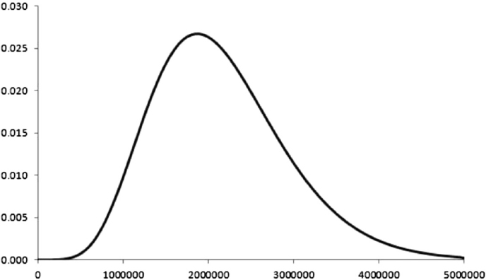
Figure 9.27. Probability usage for a single user withdrawing from a credit line of total value L = 5,000,000. The distribution parameters are specified in Table 9.30
Table 9.31. Values of the 1st and 99th percentiles U01 and U99, and of average usage ![]() , for the calculation of usage probability in Figure 9.27
, for the calculation of usage probability in Figure 9.27
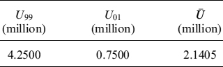
where ![]() is the i-th idiosyncratic event-counting process indicating the number of times it has jumped by time t, while NC(t) is the common event-counting process indicating the number of times it has jumped by time t; pi indicates the weight (or the probability) by which the common event affects single debtor i. So, we can either have a withdrawal specific for each debtor, or a common withdrawal for all debtors, although in the latter case every debtor has probability pi to actually withdraw.33
is the i-th idiosyncratic event-counting process indicating the number of times it has jumped by time t, while NC(t) is the common event-counting process indicating the number of times it has jumped by time t; pi indicates the weight (or the probability) by which the common event affects single debtor i. So, we can either have a withdrawal specific for each debtor, or a common withdrawal for all debtors, although in the latter case every debtor has probability pi to actually withdraw.33
To illustrate the procedure, consider for simplicity two credit lines of amounts, respectively, L1 and L2, so that the total portfolio of credit lines of the bank is L = L1 + L2. Let w1 (w2) be the value of 1% of the first (respectively, second) credit line, w1 = L1 × 1%.
Let us divide the usage percentage of the total credit line L into G discrete intervals of size δ = 1/G. For example, we divide total usage into 100 intervals from 0 to 100% of equal size δ = 1%. A given usage is assigned to each interval (e.g., usage corresponding to the midpoint or the upper bound of the interval). Let U(k) be the usage of the two lines for the interval [lk−1 × L, lk × L], where lk = kδ = k/100. The probability of usage U(k) can be expressed as
Table 9.32. Withdrawal model specification. Columns represent individual components and rows common components. Each withdrawal is a combination of jumps of two components
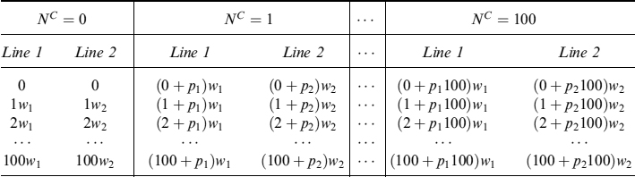

To evaluate (9.120) in practice, we can build a table like that in Table 9.32. Each column records the number of times NC the common event occurred. Given this, each row shows withdrawal from the two lines. For example, the second row in the second column shows withdrawal from line 1 when there is one idiosyncratic jump and one common jump (i.e., (1 + p1 × 1)× w1), since we only have probability p1 that the common jump actually translates into withdrawal from line 1.
The probability that each idiosyncratic jump occurs can be computed by (9.116), by setting ![]() and using the related CIR process. The probability P[NC = K] is similarly derived as in (9.116), by setting
and using the related CIR process. The probability P[NC = K] is similarly derived as in (9.116), by setting ![]() (using parameters of the corresponding CIR process) and πi = 0.
(using parameters of the corresponding CIR process) and πi = 0.
After building the matrix, we start the following procedure.
Procedure 9.4.1. Set all probabilities P(U(k)) = 0, for k = 1,…, 100.
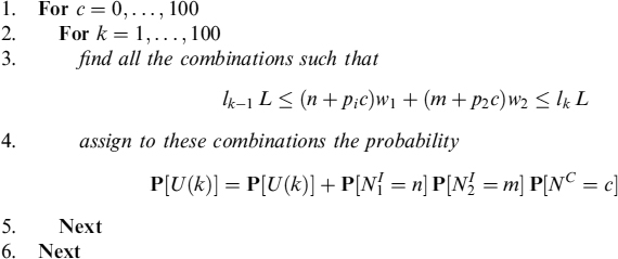
The procedure produces the discrete distribution of absolute usage U of lines L = L1 + L2.
In a compact formula, the joint probability of usage P[U(k)] for withdrawal of amount U(k) is given by
where the sum runs over all values of c, n, m that satisfy the condition lk−1L ≤ (n + p1c)w1 + (m + p2c)w2 ≤ lkL. We write this condition in compact form as
where the indicator function for an element x over a set (a, b] is
Procedure 9.4.1 can easily be generalized to the case when the bank has a portfolio of M credit lines. All the combinations that generate usage U > L have a probability that can be summed to probability P(R) in equation (9.117) (i.e., to have an overdraft on the lines). This probability can be dealt with using the normalization approach outlined in Section 9.4.3.
Example 9.4.4. We consider joint usage of a credit line from two identical credit lines, each of total value L1 = L2 = 5,000,000, using the parameters in Table 9.33. We consider extreme cases when the common process plow = 0.01 (lowly correlated) and when the common process phigh = 0.99 (highly correlated). We have chosen parameters such that both intensities have the same CIR parameters for the total process
![]()
and equate the CIR parameters used in the case of the single credit line in Example 9.4.3. The results are shown in Figure 9.28.
Marginal distributions of the usage of credit lines
For each debtor withdrawing from the total of credit lines L, we can obtain the marginal probability distribution of usage of its line by following the methods outlined in Section 9.4.3. Assuming that the i-th debtor can withdraw a maximum amount Li from the total of lines L, the marginal probability Pi[Ui (k)] of usage of the Ui(k) bucket in terms of the common and idiosyncratic distributions is

where lk = kLi/100. Equation (9.124) is obtained using Procedure 9.4.1 when only one credit line is present. Since, for a single credit line, the probability of usage for bucket Ui(k) is given by all processes with k − 1 < n + pic ≤ k, we obtain

Table 9.33. Parameters used for the joint probability of usage when phigh = 0.99 (highly correlated) and when plow = 0.01 (lowly corelated)
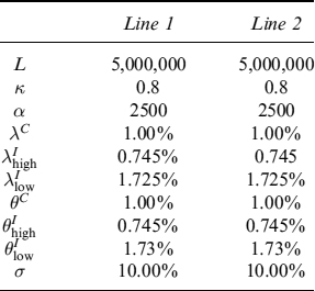
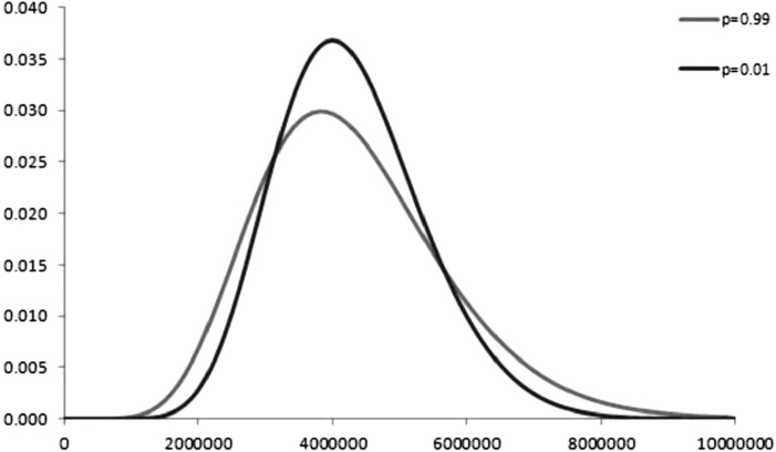
Figure 9.28. The joint probability of usage when p = 0.01 (lowly correlated) and when p = 0.99 (highly correlated), using the parameters in Table 9.33. Also shown are the averages, the 1st and the 99th percentile of the two distributions
Using the results in Section 9.4.3, the probability Pi[R] of having an overdraft on the single credit line i is
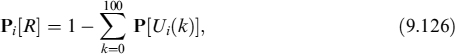
from which we obtain the normalized marginal distribution as
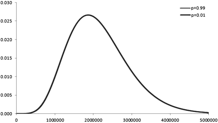
Figure 9.29. The marginal usage probability distribution for a 5,000,000 credit line, given the joint usage distribution arrived at through the parameters in Table 9.33. We show the case when there is high correlation (p = 0.99) and low correlation (p = 0.01) with the process of common usage
Example 9.4.5. In Example 9.4.4, we considered the case of the joint usage distribution of two identical credit lines, respectively with a low (p = 0.01) or a high (p = 0.99) correlation with the common withdrawal process. Here, we construct the marginal usage distributions for each credit line. The parameters are given in Table 9.33. Since correlation parameter p also occurs in the indicator function, when p = 0.01, the common jump does not affect the sum n + p c in the indicator function, and the probability of usage coincides with the idiosyncratic probability; for p = 0.99, the probability of usage is the convolution of idiosyncratic and common components. In the case considered, the two distributions coincide because we assumed the same process for intensity in both cases, see Figure 9.29.
For both p = 0.99 and p = 0.01, we find that the 99th percentile of the joint distribution lies below the 99th prcentile of two identical single credit lines. For example, for p = 0.99, the value of the 99th percentile for the joint distribution is L99,joint = 8,100,000, while each single line with the same parameters has a 99th percentile at L99,single = 4,300,000. We thus have L99,joint < 2L99,single. Similarly, for p = 0.01, the value of the 99th percentile for the joint distribution is L01,joint = 5,400,000, while each single line with the same parameters has a 99th percentile at L01,single = 3,000,000. We thus have L01,joint < 2L01,single.
Term structure of usage
We study how the probability distribution evolves in time when future times at which usage is computed are changed. We make the simplifying assumption that the borrower withdraws the line only on a predefined number of dates Tj, with j ∈ {1,…, n}. As in the examples below, we consider usage over the period of one year divided into 12 months (n = 12), and we take monthly steps
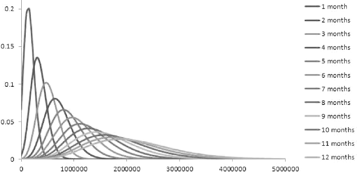
Figure 9.30. The term structure of usage probability of a single credit line, using the parameters given in Table 9.30
at which usage is computed.
Example 9.4.6. We consider the term structure of usage of a single credit line, using the parameters given in Table 9.30, and the term structure of time steps defined in equation (9.128). To model the term structure of usage numerically, we build a cycle going from j = 1 to j = 12 in which, at each step, we generate probability of usage P[N = n], at withdrawal date Tj. We obtain the plot in Figure 9.30. In Table 9.34 we show the average and the 99th percentile of the term structure of distributions.
Table 9.34. The term structure of the 1st percentile, the 99th percentile and the average usage of a single credit line arrived at through the parameters given in Table 9.30
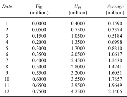
Example 9.4.7. We consider the term structure of joint usage of two identical credit lines, using the parameters given in Table 9.33, and the term structure of withdrawal dates as in equation (9.128). To model the term structure of usage numerically, we build a cycle going from j = 1 to j = 12 in which, at each step, we generate the probability of usage distribution for both the common component P[NC = c] and each idiosyncratic one P[NI = n], at time horizon Tj. Since the two lines in Table 9.33 are identical, we do not need to distinguish between the two idiosyncratic probabilities. In the case of high correlation (p = 0.99), joint usage evolves in time as shown in Figure 9.31. In the case of weak correlation (p = 0.01), we obtain the plot in Figure 9.32.
Example 9.4.8. We build the term structure of the marginal usage distribution of a credit line associated with the portfolio of credit lines in Example 9.4.4, for the case when there is high correlation with the common default probability and for the case when there is low correlation. We build a cycle going from j = 1 to j = 12 in which, at each step, we generate the probability of usage distribution for both the common component P[NC = c] and the idiosyncratic one P[NI = n], at time horizon Tj. After we normalize these distributions according to the procedure in Section 9.4.3, we find the probability of usage P[U(k)] from equation (9.124).
The term structure of the marginal distribution for the joint probability distribution in Example 9.4.7 is shown in Figure 9.33 and Table 9.35 when p = 0.99, and in Figure 9.34 and Table 9.36 when p = 0.01.
Adding default events
The intensity of default of the i-th credit line, ![]() , is related to the stochastic withdrawal intensity for the i-th borrower
, is related to the stochastic withdrawal intensity for the i-th borrower ![]() by equation (9.105), and follows the CIR process defined in equation (9.109). At time t, the probability of survival to time T is
by equation (9.105), and follows the CIR process defined in equation (9.109). At time t, the probability of survival to time T is
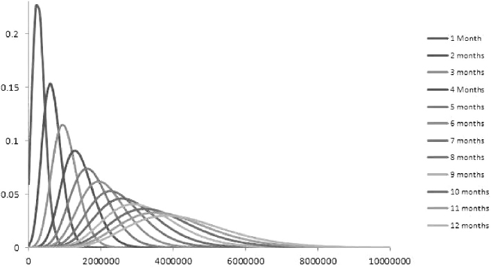
Figure 9.31. The term structure of joint usage probability of two identical credit lines when p = 0.99 and the other parameters are as in Table 9.33
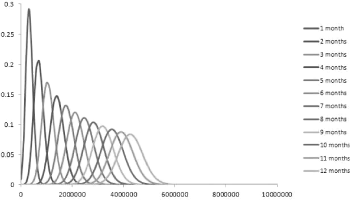
Figure 9.32. The term structure of joint usage probability of two identical credit lines when p = 0.01 and the other parameters are as in Table 9.33
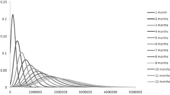
Figure 9.33. The term structure of marginal usage probability of a credit line when p = 0.99 and the other parameters are as in Table 9.33
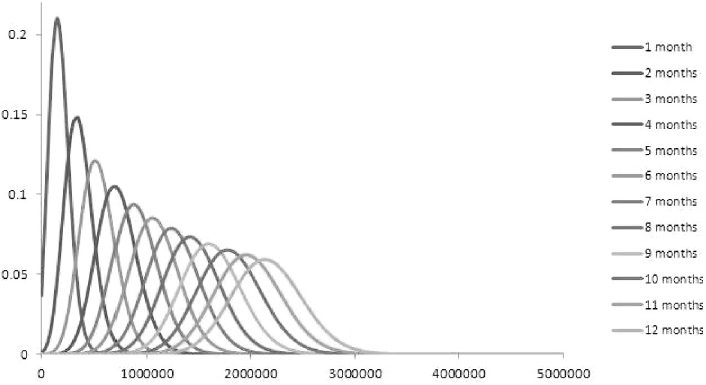
Figure 9.34. The term structure of marginal usage probability of a credit line when p = 0.01 and the other parameters are as in Table 9.33
Table 9.35. The term structure of the 1st percentile, the 99th percentile, and average usage from the marginal distribution of the usage probability of a credit line when there is high correlation (p = 0.99) with the common default probability (the parameters are given in Table 9.33)
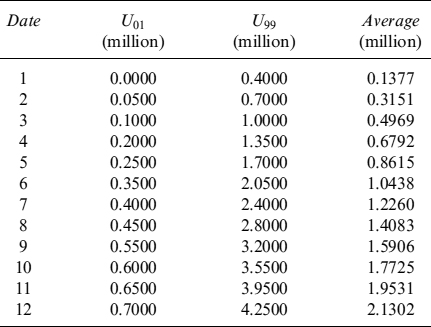
where A(t, T) and B(t, T) are functions entering the CIR discount factor defined in equation (8.27). Similarly, the probability of default is
Table 9.36. The term structure of the 1st percentile, the 99th percentile and average usage from the marginal distribution of the usage probability of a credit line when there is low correlation (p = 0.01) with the common default probability (the parameters are given in Table 9.33)
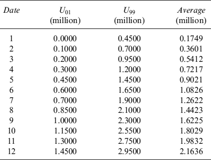
Since ![]() , we use an approximation34 to find usage in the case of default. We introduce the indicators
, we use an approximation34 to find usage in the case of default. We introduce the indicators ![]() and DC, which take the value one in the case of default and zero in the case of survival to time T. The indicator for process
and DC, which take the value one in the case of default and zero in the case of survival to time T. The indicator for process ![]() is then
is then ![]() , where ξi is one with probability Pi and zero with probability 1 − Pi. The probability of usage P[Uk] for the total credit line L, with lk−1L< Uk ≤ lkL and with a total of N credit lines, can be written as
, where ξi is one with probability Pi and zero with probability 1 − Pi. The probability of usage P[Uk] for the total credit line L, with lk−1L< Uk ≤ lkL and with a total of N credit lines, can be written as
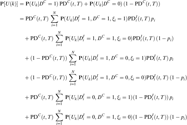
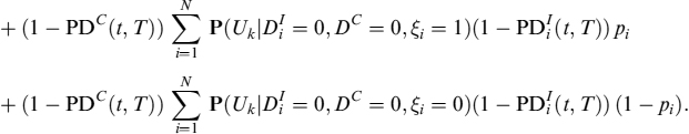
When the i-th firm defaults, its probability of usage is zero, ![]() , independently of the value of the other indicators DC and ξi. We also have a default event if both ξi = 1 and DC = 1. These cases correspond to the first five sums above, which give a probability of zero usage, while the remaining three probabilities are
, independently of the value of the other indicators DC and ξi. We also have a default event if both ξi = 1 and DC = 1. These cases correspond to the first five sums above, which give a probability of zero usage, while the remaining three probabilities are
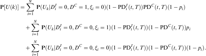
The three terms in the summation correspond to default of the common line with ξi = 0 (with probability 1 − pi, first line in the equation) and to survival of both the idiosyncratic and common terms (last two lines of the equation).
In case of no default of the i-th line, all three probabilities ![]() ,
, ![]() ,
, ![]() ,
, ![]() are equal and equate to the probability of usage computed without assuming default, call it P(Uk, Di = 0), where Di is a new indicator that states whether the i-th firm has defaulted or not at time T, independently of the cause. Summing up all three probabilities, we obtain the idiosyncratic usage from the i-th line including the survival probability,
are equal and equate to the probability of usage computed without assuming default, call it P(Uk, Di = 0), where Di is a new indicator that states whether the i-th firm has defaulted or not at time T, independently of the cause. Summing up all three probabilities, we obtain the idiosyncratic usage from the i-th line including the survival probability,
Similarly, we define
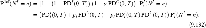
Joint usage with probability of default
We now introduce the possibility that the entirety of credit lines L is drawn by two defaultable debtors. The case of m users can easily be derived from this case. To obtain the joint usage from two credit lines, we modify equation (9.121) as
with the triplet (c,n,m) satisfying lk−1L ≤ (n + p1c)w1 + (m + p2c)w2 ≤ lkL, lk = k/100, wi = Li/100.
To obtain the marginal probability of usage from a single credit line of total usage Li, we modify equation (9.124) by considering the idiosyncratic probability of default Psurv[NI = n] in equation (9.131) for the idiosyncratic process. We have

where the suffix “def” indicates that the probability distribution takes into account the probability of default.
Example 9.4.9. In Figure 9.35, we show the results for the joint probability of usage for two credit lines using the parameters in Table 9.33, obtained from equation (9.133). We considered the case when there is low correlation with the common default process (p = 0.01) and the case when there is high correlation with the common default process (p = 0.99). Figure 9.35 further compares the joint probability of usage without considering the probability of default, equation (9.121). We have collected the relevant information on the distributions in Table 9.37 and in Table 9.38 we show the term structures of expected usage for all the cases..
The marginal probability distribution for a single credit line of the joint distribution considered above is shown in Figure 9.36 and Table 9.38 for both cases p = 0.01 and p = 0.99. Figure 9.36 further shows the marginal usage probabilities when the probability of default is not considered, equation (9.124). We find the probability of zero usage for p = 0.99 equal to Pdef(0) = 1.94%, and for p = 0.99 equal to Pdef(0) = 1.72%.
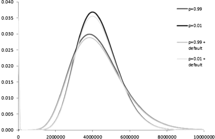
Figure 9.35. The joint usage probability of two credit lines for p = 0.99 and p = 0.01 and the corresponding joint usage probability including the probability of default for p = 0.99 and p = 0.01
Table 9.37. Relevant data for the distributions in Figure 9.35
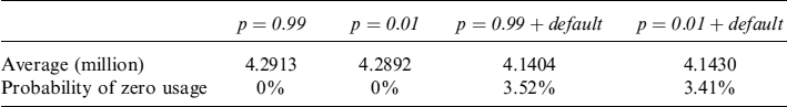
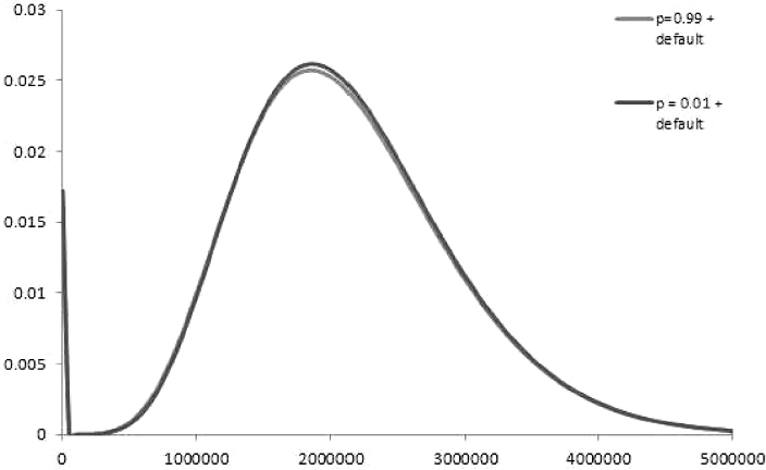
Figure 9.36. The marginal usage probability for a single credit line using the parameters as in Table 9.33 for the case of high correlation (p = 0.99) and that of low correlation (p = 0.01) with the common default process
9.4.4 Pricing of credit lines
The setup we introduced above is useful to monitor the withdrawal distribution of a portfolio of credit lines and thus allow for effective liquidity management. Nonetheless, it is also rich enough to allow pricing of a credit line featured by a notional amount of L, by a probability of usage P[U] and by a term structure of usage at times Tj, j ∈ {1,…, n}, defined in Section 9.4.3. We indicate average usage of the credit line up to time Tj with ![]() , the liquidity buffer with LBi and we define
, the liquidity buffer with LBi and we define
where T0 = t.
Assume that at time Tj the funding cost (expressed as a simply compounded rate ) that the bank has to pay for the period [Tj−1, Tj] is a sum of constant funding spread sB and risk-free rj, the latter derived from the term structure of risk-free35 discount factors by
Table 9.38. Average usage with the parameters in Table 9.33, for p = 0.99 and p = 0.01. We also separately show the case of no default (first two columns) and the case of default (last two columns)
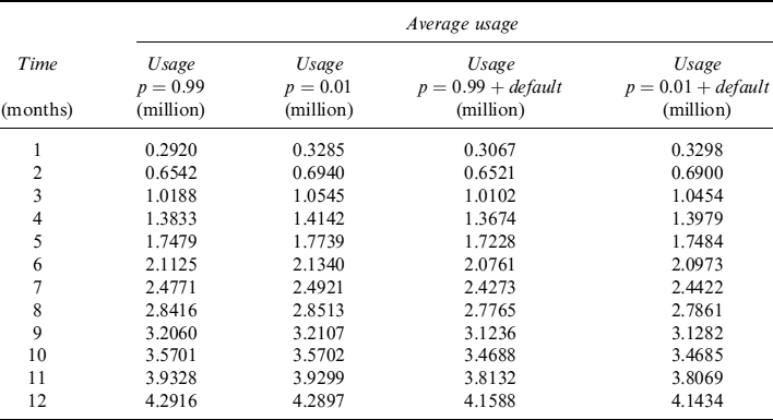
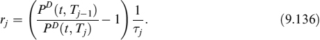
Let us define total usage of the credit line as:
Absolute usage Uj is split into three parts:
- Expected (average) usage
 .
. - Liquidity buffer LBj to cope with usage beyond the expected level.36
- A liquidity option,
 , sold to the borrower equal to the maximum usage the bank can cover (expected plus LB) minus actual usage U.
The LB is set at a level that covers maximum usage in excess of the expected level at a given confidence level (say, 99%).
Expected usage, given that maximum usage is within the confidence level chosen when setting the LB, can be found with the formula:
which makes use of the distribution of usage derived above.
When a counterparty withdraws a given amount from the line, it will pay interest for the period. Just for modelling purposes, we assume that the borrower decides to use the line at the beginning of each period (Tj−1) and repays the amount plus interest at Tj; then it can choose to withdraw a given amount from the credit line for all periods until expiry of the contract.
Assume for the moment that the borrower is not subject to credit risk, so that the bank does not have to worry about being compensated for the default. The interest required should only be enough to cover the total funding cost of the bank (i.e., the risk-free rate plus the bank's funding spread). Over the period [Tj−1, Tj] the bank can expect to receive interest equal to:
which is simply the total funding cost charged for the duration of the period for expected usage (given maximum usage).
Given maximum usage of the line at time Tj, at a confidence level that we assume the bank sets at 99%, the liquidity buffer is:
where U99,j is the 99th quantile of the distribution at time Tj. Total usage in equation (9.137) is
usage up to the value U99,j is
So, expected interest received, given maximum usage of the credit line at the 99% c.l., is
9.4.5 Commitment fee
In credit line contracts the bank applies a fee that has to be paid periodically by the counterparty. This fee remunerates the bank for providing liquidity on demand and is applied to the unused part of the line: The level of the fee can be determined in such a way that the contract is fair at inception, as we explain below.
The bank funds maximum usage of the credit line over period Tj by borrowing quantity U99,j at time Tj−1, and repaying the amount [1 + Tj(rj + sB)] U99,j (i.e., notional plus total funding cost at time Tj). This amount should equate to earnings from:
- Expected interest received (as given in equation (9.143)) and repayment of the amount withdrawn.37
- Reinvesting the unused amount
 in risk-free liquid investments earning rj.
 - The commitment fee Feej applied to the unused amount
 .
.
from which, using equation (9.143), we obtain the fair commitment fee
Introducing the fee rate cj for the commitment fee over the unused amount,
and equating equations (9.145) and (9.146), we obtain
The commitment fee is determined once and for all at the inception of the contract, so we need to find the unique rate c that ensures the present value of the total amount paid by the bank over all periods [Tj−1, Tj], until the expiry of the contract, equates to the present value of inflows previously described, received from all periods [Tj−1, Tj] as well. We then have:

where PD(t, Tj) is the risk-free discount factor for cash flows occurring at Tj.
An example should clarify the ideas presented so far.
Example 9.4.10. We consider the term structure of a single credit line using the parameters in Table 9.30. In Table 9.39, we give values for U99, average usage up to ![]() , average unused line
, average unused line ![]() , and commitment rate cj for usage of the single credit line, obtained from equation (9.147). We used the value sB = 1%, over a period of a year divided into n = 12 months. The unique rate ensuring that bank ouflow and inflow equate, equation (9.148), is c = 0.3%.
, and commitment rate cj for usage of the single credit line, obtained from equation (9.147). We used the value sB = 1%, over a period of a year divided into n = 12 months. The unique rate ensuring that bank ouflow and inflow equate, equation (9.148), is c = 0.3%.
Table 9.39. Values for the 99th percentile (U99), usage up to ![]() , unused line
, unused line ![]() and the commitment fee rate cj for a single credit line, obtained from equation (9.144) using the parameters in Table 9.30. We assumed sB = 1% and chose the other parameters from Table 9.30
and the commitment fee rate cj for a single credit line, obtained from equation (9.144) using the parameters in Table 9.30. We assumed sB = 1% and chose the other parameters from Table 9.30
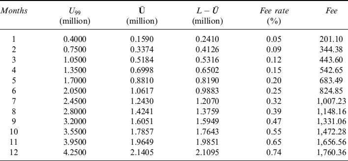
9.4.6 Adding the probability of default
We consider the pricing of a credit line subject to default risk of the borrower over the life of the contract and relating to the term structure of usage described in Section 9.4.4. When the possibility of default is taken into account, the expected value of usage U in equation (9.142) is computed using the probability of usage Pdef [U] (see equation (9.134)) in place of P[U]. Put mathematically,
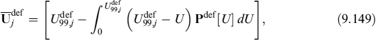
where ![]() is the 99th quantile of
is the 99th quantile of ![]() at time Tj.
at time Tj.
For the i-th credit line, the probability of withdrawal Pdef[U] is given by equation (9.134), whereas the probability the line has survived to time Tj−1 is
When the possibility of default is not considered, balancing between the costs of the bank and the corresponding profits leads to equation (9.144). To find an analogy to equation (9.144) when the probability of default is included, we have to consider that expected interest and the commitment fee are repaid in the case the borrower survives, while in the case of default the bank receives only recovery amount ![]() . To compensate for this risk, the bank adds credit spread sc to the total interest applied over the average used amount. Put mathematically,
. To compensate for this risk, the bank adds credit spread sc to the total interest applied over the average used amount. Put mathematically,
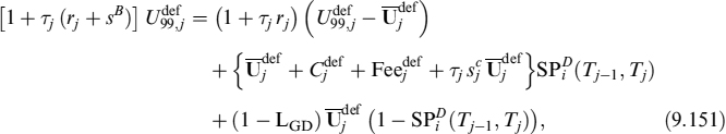
where the expected interest earned by the bank is
the commitment fee is
Equation (9.151) states that the total funding cost plus repayment of the capital ![]() equates to:
equates to:
- The interest earned by investing the unused amount in a risk-free liquid asset:
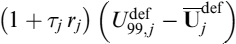
- The expected amount received from the counterparty in case it survives:
 .
. - Recovery of the used amount in case the counterparty defaults:
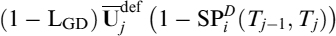 .
.
The credit spread that the bank should apply, ![]() , satisfies
, satisfies
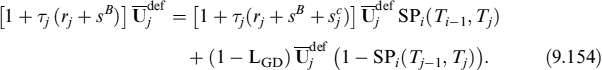
So we find:
Furthermore, in this case the bank does not apply different spreads for each period, but sets at inception a single spread valid for the entirety of the contract, ![]() , which is determined as:
, which is determined as:
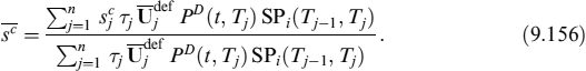
The commitment fee has to be recalculated considering the probability of default of the borrower: using equation (9.151) we obtain an expression for fee rate cj over period Tj as:
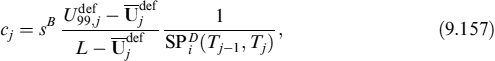
to be compared with the value in equation (9.147) obtained when the probability of default is not added. The unique value of c that has to be applied for the entire duration of the contract is:
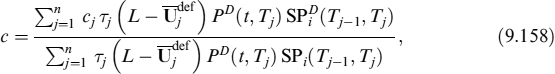
Example 9.4.11. Referring to the discussion in Example 9.4.10, in Table 9.40 we show the value of the fee rate for usage of a single credit line when the probability of default is added. The probability of default is modelled by a CIR process using the parameters in Table 9.30.
The numerical value of the fee rate in equation (9.158) is c = 0.30% and the credit spread in equation (9.156) is ![]() .
.
9.4.7 Spread option
The fact that the credit spread for the borrower is set once for the entire life of the contract at inception implicitly means that the bank is selling a spread option to the counterparty. The borrower will find it attractive to withdraw the line if its credit-worthiness worsened, since it can always pay the spread fixed in the contract. This is the reason we introduced a dependenc of the withdrawal intensity of the line on the probability of default of the borrower: this contributes to building the marginal and joint distribution of withdrawals and as such it is useful for liquidity management purposes. On the other hand, the bank has not yet considered how much the option is worth financially, so we now have to include in the pricing.
Table 9.40. Values for the 99th percentile (U99), usage up to ![]() , unused line
, unused line ![]() and the commitment fee rate cj for a single credit line, obtained from equation (9.144) using the parameters in Table 9.30. We assumed sB = 1% and chose the other parameters from Table 9.30
and the commitment fee rate cj for a single credit line, obtained from equation (9.144) using the parameters in Table 9.30. We assumed sB = 1% and chose the other parameters from Table 9.30
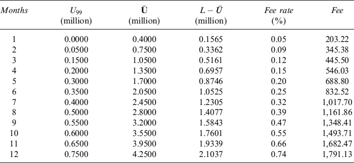
For a given time Tj, the payout of the spread option to the counterparty is:
The payoff is the same as a call option on the level of the credit spread where the strike ![]() is the value that satisfies equation (9.157) (i.e., the level of the credit spread set for the entire duration of the contract). The value is obviously greater when the credit spread increases with respect to the strike level, since the borrower finds it more convenient to withdraw the line rather than borrowing money by a new debt contract.
is the value that satisfies equation (9.157) (i.e., the level of the credit spread set for the entire duration of the contract). The value is obviously greater when the credit spread increases with respect to the strike level, since the borrower finds it more convenient to withdraw the line rather than borrowing money by a new debt contract.
To compute equation (9.159), we replace the expectation value by weighted integration over the possible values of default intensity λ, where the weight pi(λ) is the CIR probability of obtaining a value λ at time Tj if the value at time t is λt. Mathematically, the probability is
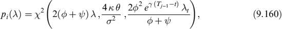
where
The spread option formula is
where we have made the dependence of usage U and sc on λ explicit. Looking at this in greater detail, sc(λ) depends on λ through survival probability SPi(Tj−1, Tj), as is clear from (9.157). The term ![]() limits the range of integration to
limits the range of integration to ![]() , where
, where
![]() is the value of λ at time Tj that satisfies
is the value of λ at time Tj that satisfies
Usage U(λ) depends on λ through the probability distribution of the Poisson process Pdef [N = k], see equation (9.134), and the relation between the probability of the i-th debtor ![]() making a withdrawal and default of the i-th credit line expressed in equation (9.105). Conditioning the probability of usage to
making a withdrawal and default of the i-th credit line expressed in equation (9.105). Conditioning the probability of usage to ![]() gives
gives

where Uk = kL/100.
The spread option is sold by the bank to the counterparty, so it is an additional cost that has to be considered besides total funding, for each period the life of the contract has been divided into. We charge this additional cost ![]() to the commitment fee in equation (9.151), by solving the following equation:
to the commitment fee in equation (9.151), by solving the following equation:
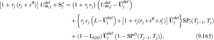
where ![]() satisfies equation (9.154). We obtain
satisfies equation (9.154). We obtain
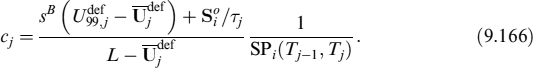
To compute the value of the spread option, we use a numerical approximation of the integral over λ in equation (9.164). We first truncate the range of integration to ![]() , we divide the interval
, we divide the interval ![]() into N intervals, setting
into N intervals, setting
and we define integration points ![]() . Equation (9.164) is then approximated as
. Equation (9.164) is then approximated as

Example 9.4.12. In Table 9.41, we show spread options ![]() , fee rate cj and the commitment fee for a single credit line using the parameter in Table 9.30. Using equation (9.158) with the values of cj as in equation (9.166), we obtain the new value c = 0.42%, higher than c = 0.30% obtained without considering spread options.
, fee rate cj and the commitment fee for a single credit line using the parameter in Table 9.30. Using equation (9.158) with the values of cj as in equation (9.166), we obtain the new value c = 0.42%, higher than c = 0.30% obtained without considering spread options.
Table 9.41. Values for spread option ![]() , fee rate cj and the commitment fee for a single credit line with parameters chosen as in Table 9.30
, fee rate cj and the commitment fee for a single credit line with parameters chosen as in Table 9.30
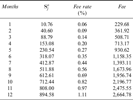
9.4.8 Incremental pricing
The pricing of a credit line is strongly affected by considering it as a new contract to be included in the existing portfolio of credit lines, but not on a standalone basis, as we have done above: we call this incremental pricing. Here the correlation effect can play a role in making the portfolio more diversified so that the bank can close the contract by giving better terms to the counterparty, thus being competitive with other financial institutions without impairing the correct and sound remuneration for all the costs and risks borne.
Consider joint usage of a portfolio of credit lines with total notional L opened by the bank to m debtors, so that
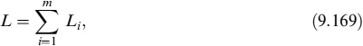
where Li is maximum usage of the i-th line. Because of the subadditivity of the quantile, the 99th percentile of the distribution U99(L1,…, Lm) and the 99th percentiles of each marginal distribution U99,i satisfy
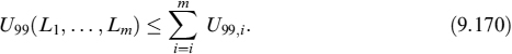
When we consider the single lines of m separately, a buffer needs to be allocated that is higher than the one implied by the joint distribution of usage of the lines. If pricing of a new line is operated on a standalone basis, this will result in commitment fees having higher values. If the bank wants to improve the level of the fee to the borrower, it may consider what happens when inserting the new contract into the existing portfolio. Consider the following incremental quantile approach for usage of credit lines:
the 99th percentile of the joint distribution satisfies
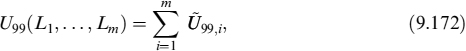
so that U99(L1,…, Lm) is additive in the incremental quantile. To determine the value of U99,I for a particular counterparty I, we proceed by first computing the 99th percentile of the distributionof joint usage in which the I-th debtor has maximum usage ![]() , with
, with ![]() . We then compute the numerical derivative
. We then compute the numerical derivative
This is the increment of the maximum level, at the 99% c.l., of total usage of all credit lines. This increment can be attributed to the new contract the bank is dealing with the counterparty. It is also the level to use in the formulae we presented above for standalone pricing, replacing the maximum usage level at the 99% c.l. derived from the distribution of the single line considered separately from the portfolio. The commitment fee is then calculated accordingly.
Example 9.4.13. We consider the joint usage probability of two users of total credit lines of, respectively, L1 = 5,000,000 and L2 = 7,000,000. The parameters for usage probabilities are given in Table 9.42. We price the marginal probability distribution for the first credit line of total usage L1 = 5,000,000. Table 9.43 summarizes pricing of the credit line without considering the incremental quantile of usage.
In Table 9.44, we reprice the credit line on an incremental basis by using the value of ![]() instead of U99,j with all other details of the distribution left unchanged.
instead of U99,j with all other details of the distribution left unchanged.
In Table 9.45, we summarize the results to ascertain the value of the unique fee rate c obtained whether we consider the spread option or not and whether or not we reprice the marginal credit line distribution with the incremental liquidity buffer.
Table 9.42. Parameters used to build the marginal joint usage distribution for two credit lines when there is high correlation phigh = 0.99 (see Example 9.4.13)
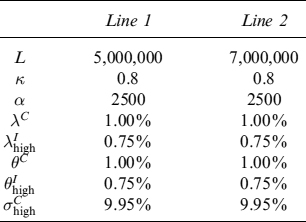
Table 9.43. The values of ![]() ,
, ![]() , the fee rate and the commitment fee for the marginal joint usage distribution using parameters from Table 9.33 and phigh = 0.99
, the fee rate and the commitment fee for the marginal joint usage distribution using parameters from Table 9.33 and phigh = 0.99
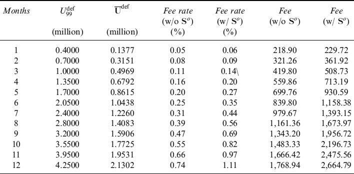
Table 9.44. The values of ![]() ,
, ![]() , the fee rate and the commitment fee for the marginal joint usage distribution (from incremental pricing) using parameters from Table 9.33 and phigh = 0:99
, the fee rate and the commitment fee for the marginal joint usage distribution (from incremental pricing) using parameters from Table 9.33 and phigh = 0:99
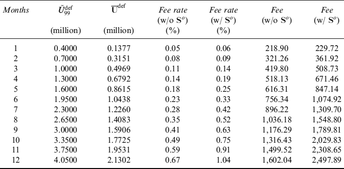
Table 9.45. The values of fee rate c when there is no spread option, when there is a spread option and when there is standalone (LB = U99) and incremental ![]() pricing
pricing
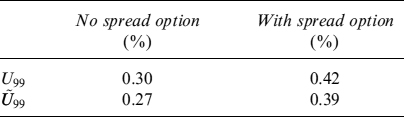
APPENDIX 9.A GENERAL DECOMPOSITION OF HEDGING SWAPS
Assume at time t0 the mortgage has the following contract terms:
- The mortgage notional is A0 = A.
- The mortgagee pays on predefined scheduled times tj, for j ∈ (0, 1,…, b), fixed rate c computed on the outstanding residual capital at the beginning of reference period Tj = tj − tj−1, denoted by Aj−1. The interest payment will then be cTjAj−1.
- On the same dates, besides interest, the mortgagee also pays Ij, which is a portion of the outstanding capital, according to an amortization schedule.
- Expiry is time tb = T.
- The mortgagee has the option to end the contract by prepaying on payment dates tj the remaining residual capital Aj, together with the interest and capital payments as defined above. The decision to prepay, for whatever reason, can be taken at any time, although actual prepayment occurs on scheduled payment dates.
The assumption that the interest, capital, and the prepayment dates are the same, can easily be relaxed.
The fair coupon rate c can be computed by balancing the present value of future cash flows with the notional at time t0:
![]()
which immediately leads to:
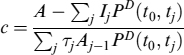
where PD(t0, tj) is the discount factor at time t0 for date tj. It should be noted that the quantity A − ∑jIjPD(t0, tj) can be replaced by ∑jTjAj−1Fj(t0)PD(t0, tj),38 where Fj(t0) is the forward at time t0 starting at time tj.
When projecting expected cash flows, the probability of an anticipated inflow of the residual notional at given time tk has to be computed as follows:
where SPe(t, T) is the survival probability. Expected total cash flow (interest + capital) at time t0 for each scheduled payment time39 {tj = tk} is given by the formula:
The expected outstanding amount at each time is given by:
Let us consider hedging this mortgage with a bundle of single-period swaps, starting from t0 up to tb = T:
It is possible to show, with some manipulation, that at time t1 we have:

and at t2:

where we have defined ΔPPi = PPe(t0, ti) − PPe(t0, ti−1). By the same token, at time tj we can write:
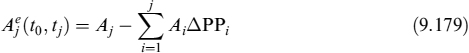
Let us now define a set of swaps with variable notional equal to the contract-amortizing schedule of mortgage SwpA(ta, tb): these swaps do not have to start at the same date as the mortgage, they can also start at later dates, in which case their notional amounts match the contract-amortizing schedule of the mortgage for residual dates only.
If we replace ![]() in the hedging portfolio, we sum over all the forward-starting swaps, we see that the portfolio actually contains:
in the hedging portfolio, we sum over all the forward-starting swaps, we see that the portfolio actually contains:
- a fixed rate payer swap SwpA(t0, tb);
- a portfolio of short-payer (or long-receiver) forward-starting swaps, each ending in tb and each rescaled to a given factor:
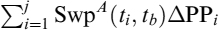 .
.
Each forward-starting swap can be, in turn, decomposed by means of put–call parity: SwpA(ti, tb) = PayA(ti, tb; c) − RecA(ti, tb; c). The payer and the receiver are written on swaps mirroring the mortgage contract-amortizing schedule for the residual dates until the final date tb. So, collecting all the results again, we have that hedging portfolio P is equal to

This is the result described in Section 9.2.3.
APPENDIX 9.B ACCURACY OF MORTGAGE RATE APPROXIMATION
In this section we simulate risk-neutral distribution and assume lognormal forward rates with the purpose of getting a good approximation of counterparty risk which would otherwise be computed via the yield curve simulation of an internal model.
The cost borne when a mortgage is prepaid can be considered equal to the unwinding cost of a hedging swap that matches cash flows perfectly. Assuming there is no credit spread due to the default risk of the mortgagee, the swap rate is equal to the mortgage rate. EL can thus be measured as the expected positive exposure (EPE) of a hedging swap.
The assumption of lognormal forward rates also allows for a closed-form approximation to be used for the EPE of a swap contract (equal to EL of the mortgage on possible prepayment dates): we test the accuracy of the closed-form formula with respect to Monte Carlo calculation of the EPE.
9.B.1 Internal model simulation engine
We calibrated the zero curve to swap rates (pillars 1 to 10, 15, 20, 25 and 30) on each day from 2 September 1998 to 15 August 2009. For each day we then computed the 30 adjacent forward Libor rates with maturity 1 year. We then calculated percentage daily change for the panel including the 30 adjacent forward rates.
In Figure 9.37 we plot the 10Y swap over the entire period. In Figure 9.38 (left-hand side), we plot the historical annualized volatility of forward rates and on the right-hand side we plot the average correlation between all forward rate pairs with the same start date distance. On the right-hand side, we can clearly see a decay pattern going on: the more distant the start date of forward rates the smaller their correlation on average.
We next simulated the EPE for a 10-year 5% payer swap (pay fixed 5%, receive floater). We simulated the evolution of the risk-free curve using a multifactor Libor market model where the annualized volatility of forward rates is constant for all start dates at 20% (in line with Figure 9.38, left-hand side), and the correlation between any two forward rates ri and rj (where ti and tj are the start dates of the two forward rates) is modelled as
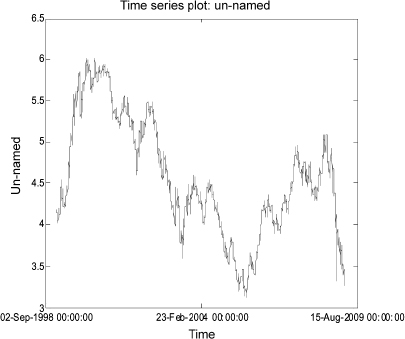
Figure 9.37. Time series of the 10-year euro swap
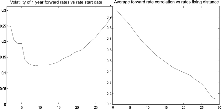
Figure 9.38. Forward rate volatilities (left-hand side) and average correlation (right-hand side)
where the coefficient 0.95 has been calibrated to fit the decay displayed in Figure 9.38 (right-hand side).
In our simulation exercise we will model evolution of the mark-to-market of a plain vanilla swap through time. To do so we will simulate evolution of the forward rate curve given an initial forward curve, a deterministic and constant forward rate volatility term structure and a deterministic and constant correlation between forward rates as calculated in equation (9.181).
9.B.2 Results
Figures 9.39, 9.40 and 9.41 compare the analytical approximation of the EPE vs the simulated EPE for different sets of simulation scenarios in the event of a plain vanilla (non-amortizing) swap:
- Different initial shapes of the forward rate curve:
- flat forward rate curve at the 5% level;
- increasing the forward rate curve from 2% for the (0Y × 1Y) forward to 5% for the (9Y × 1Y) forward.
- Different initial shapes of forward rate volatility:
- flat term structure of forward rate volatility at 20%;
- decreasing the volatility of forward rates from 20% for the 1Y to 10% for the 20Y.
- Different correlation of future Libor rates depending on their fixing date distance:
- high correlation, 95%, in line with Figure 9.38;
Figure 9.39. Analytic (light-grey line) and simulated EPE (black line) for a 10Y plain vanilla swap. (Left) Flat forward curve at 5% level, flat term structure of forward rate volatility at 20% and annual forward rate correlation decay equal to 99%. (Right) Forward rate curve from 2% for the (0Y × 1Y) forward to 5% for the (9Y × 1Y) forward; the term structure of forward rate volatility is flat at the 20% level and annual forward rate correlation decay equal to 99%. The number of simulations is 10,000
Figure 9.40. Analytic (light-grey line) and simulated EPE (black line) for a 10Y plain vanilla swap. (Left) Decreasing volatility of forward rates, from 20% for the 1Y to 10% for the 20Y; annual forward rates correlation decay equal to 99% and the forward rate curve is flat at 5%. (Right) Annual forward rate correlation decay equal to 80%, flat forward rate curve at 5% and flat volatility term strucutre of 20%. The number of simulations is 10,000
- low correlation, 80%, so as to test the approximation vs more complex forward rate term structures.
- high correlation, 95%, in line with Figure 9.38;
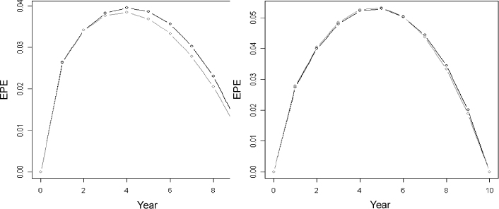
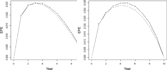
Figures 9.43, 9.44 and 9.45 are the equivalent of Figures 9.39, 9.40 and 9.41 in the event of an amortizing swap, the amortization schedule of which is depicted in Figure 9.42.
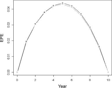
Figure 9.41. Analytic (light-grey line) and simulated EPE (black line) for a 10Y plain vanilla swap. Increasing forward rate curve, from 2% for the (0Y × 1Y) forward to 5% for the (9Y × 1Y) forward and decreasing volatility of forward rates, from 20% for the 1Y to 10% for the 20Y. The number of simulations is 10,000
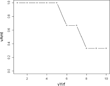
Figure 9.42. Amortization scheme for a 10Y swap
We see that the analytical approximation is satisfactory even when the initial shape of the forward rate curve, volatility term structure and forward Libor correlation are put under stress. Keeping in mind that from the regulatory standpoint the horizon of the EPE can only be up to 1 year, the analytical approximation is almost perfect.
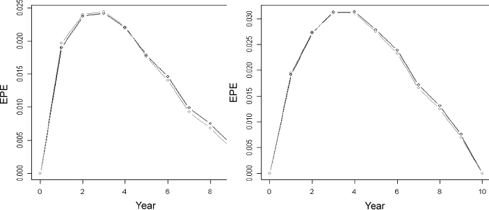
Figure 9.43. Analytic (light-grey line) and simulated EPE (black line) for a 10Y amortizing swap. (Left) Flat forward curve at 5% level, flat term structure of forward rate volatility at 20% and annual forward rate correlation decay equal to 99%. (Right) Forward rate curve from 2% for the (0Y × 1Y) forward to 5% for the (9Y × 1Y) forward; the term structure of forward rate volatility is flat at the 20% level and annual forward rate correlation decay equal to 99%. The number of simulations is 10,000
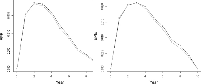
Figure 9.44. Analytic (light-grey line) and simulated EPE (black line) for a 10Y amortizing swap. (Left) Decreasing volatility of forward rates, from 20% for the 1Y to 10% for the 20Y, annual forward rate correlation decay equal to 99% and the forward rate curve is flat at 5%. (Right) Annual forward rate correlation decay equal to 80%, flat forward rate curve at 5% and flat volatility term structure of 20%. The number of simulations is 10,000
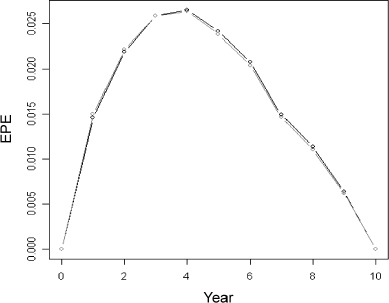
Figure 9.45. Analytic (light-grey line) and simulated EPE (black line) for a 10Y amortizing swap. Increasing forward rate curve, from 2% for the (0Y × 1Y) forward to 5% for the (9Y × 1Y) forward and decreasing volatility of forward rates, from 20% for the 1Y to 10% for the 20Y. The number of simulations is 10,000
APPENDIX 9.C ACCURACY OF THE APPROXIMATED FORMULA FOR CORRELATED MORTGAGE RATE AND PREPAYMENT INTENSITY
As mentioned above, we use an approximation to calculate the ELoP analytically, since the assumption of a correlation between the mortgage rate and prepayment intensity does not allow for a closed-form formula and we do not want to use Monte Carlo simulation.
The approximation formula has been tested against Monte Carlo simulation to test its accuracy. In the test we used the following values for CIR intensity:
- θ = 0.07
- λ0 = 0.11
- κ = 2
- ν = 0.1.
Tests were conducted assuming a generic lognormally distributed process (such as the one we chose to describe the mortgage rate) for the underlying asset and we price a call option. The volatility of the process is σ = 0.2 and the starting value of the asset is S0 = 100. The test was carried out for different values of strike K, expiry T and correlation with the CIR process ρ.
Numerical results are given in Tables 9.46–9.48.
Table 9.46. In this table we summarize and list all the values computed by Monte Carlo simulation and by the theoretical approximated formula for an European call option with stochastic prepayment intensity and expiry over 1 year. We have the following parameter specification: underlying S0 = 100 and volatility σ = 0.2
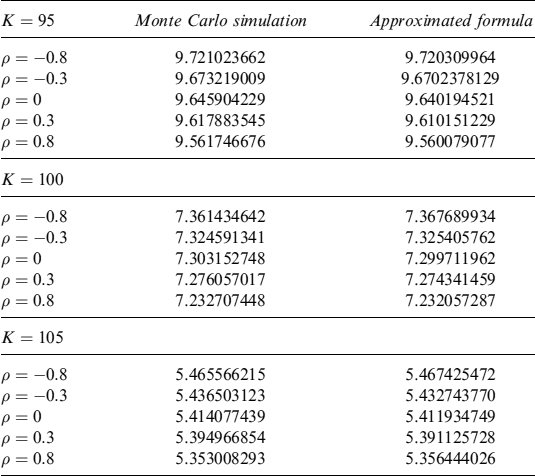
Table 9.47. In this table we summarize and list all the values computed by Monte Carlo simulation and by the theoretical approximated formula for an European call option with stochastic prepayment intensity and expiry over 5 years. We have the following parameter specification: underlying S0 = 100 and volatility σ = 0.2
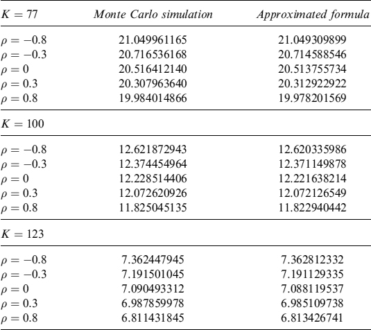
Table 9.48. In this table we summarize and list all the values computed by Monte Carlo simulation and by the theoretical approximated formula for an European call option with stochastic prepayment intensity and expiry over 10 years. We have the following parameter specification: underlying S0 = 100 and volatility σ = 0.2
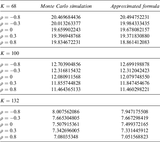
APPENDIX 9.D CHARACTERISTIC FUNCTION OF THE INTEGRAL 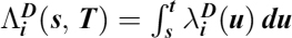
Let us consider a general process: the case in Section 9.4.3 is a special case of this process. A stochastic process X on a filtrated probability space ![]() , is said to follow CIR dynamics if it has the following form
, is said to follow CIR dynamics if it has the following form
where Wt is ![]() -standard Brownian motion and Jt is an independent compound Poisson process with jump intensity l and exponentially distributed jumps with mean μ. We want to evaluate the following expectation
-standard Brownian motion and Jt is an independent compound Poisson process with jump intensity l and exponentially distributed jumps with mean μ. We want to evaluate the following expectation
where functions α(t) and β(t) solve Riccati's equations
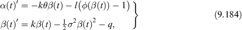
with boundary condition α(0) = β(0) = 0. The closed formula is given by
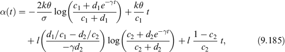
and
where
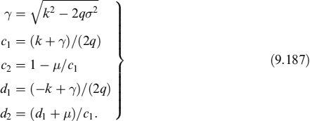
It is now sufficient to pose q = u, for ![]() , to obtain the characteristic function of the Xt process.
, to obtain the characteristic function of the Xt process.
1 The original Richard and Roll model was conceived for MBS. S = 0 if the model is used for standard mortgage portfolios.
2 What is more, some vendors advocate such a practice to bring about more competitive rates for mortgages than those of other banks. Needless to say, banks are giving away value if this policy is adopted, as we will show below.
3 Actually, the ALM should match the basis point sensitivities of the assets and liabilities for each relevant maturity bucket. We do not go into detail since they are beyond the scope of the current analysis.
4 Here we assume no transaction costs; hence, brute force replacement of the first swap by the second is chosen. Clearly, more cost-effective rebalancing strategies could be adopted to minimize transaction costs, since they are actually paid in the market.
5 Actually, after one year it is the 9Y maturity. For the purposes of this analysis we try to project the new 10Y rate.
6 It could be deterministically time dependent though.
7 This very important distinction is not manifest in this simplified 2-year example, but it is much clearer by generalizing (see Appendix 9.A) the suggested decomposition of the hedge using arbitrary maturities and amortization schedules.
8 The model was proposed in [47].
9 Basically, parameter ψ is assumed to be included in parameter κ. They both occur in formula (9.3) (always as a sum), so they can jointly be estimated from historical data. We will also use the real measure for pricing; hence, we implicitly assume that the market premium for prepayment risk is zero so that the risk-neutral measure coincides with the real one.
10 Decisions to prepay depend on the jump occurrence modelled by intensities.
11 This is trivially obtained by considering the pricing equation of an amortizing floating rate mortgage.
12 We will use the notation ca,b(t) to indicate the time-t fair rate of a mortgage with residual payments at tj, with j ∈ {a, a + 1, …, b}.
13 OIS (or Eonia for the euro) can be considered risk-free rates for practical purposes.
14 See Chapter 8 for details on market models.
16 Derivation of the formula follows [81] in the specific case when the underlying asset is a pure martingale. Extensive tests on the accuracy of the formula using Monte Carlo simulation are shown therein.
17 See [52] for complete derivation of the following formulae.
18 For more details on how to compute conditional expected values in a VaR context see [48].
19 The complete proof is in [52].
20 Scheduled payment times are assumed to be equal to possible prepayment times.
21 We would like to thank Francesco Manenti for the help preciously provided in implementing and testing the models outlined in this section.
22 We will extend the analysis of the funding mix in Chapter 11.
23 We think the term OAS is misleading for a number of reasons: it does not explicitly model any optionality and does not adjust any spread, as will be clear from what we show below. The name is likely derived from suspect practice in the fixed income market, which uses an effective discount rate to price assets by taking into account embedded optionalities (whence the name).
24 See, amongst others, [86], [57], [80] and [26].
25 The gamma function was also chosen for the behavioural function in [97].
26 See Chapter 8 for discretization schemes for CIR processes.
27 Data are also available at www.bancaditalia.it
29 We are aware this is likely not the most sound way to interpolate GDP data, but we think it is reasonably good for the limited purpose of our analysis.
30 The specification of default intensity is the same as in [60].
31 See Section 8.4.
32 See Appendix 9.C.
33 As noted in [60] and analogously for the “default” event, the approximation overestimates the number of occurrences since the sum of the idiosyncratic and common jumps can be above 100. On the other hand, it underestimates the probability of events related to multiple common events. The two effects somehow cancel each other out.
34 The approximation was first suggested in [60] and has already been used in Chapter 8.
35 As noted several times already, the best approximation to the risk-free rate is given by the OIS (Eonia for the euro) swap rates.
36 See Chapter 7 for a discussion on how to set the LB for credit lines.
37 Remember, this is only a modelling assumption that might not actually occur in reality. It allows for the amount to be repaid and immediately withdrawn again.
38 This is trivially obtained by considering the pricing equation of an amortizing floating rate mortgage.
39 Scheduled payment times are assumed to be equal to possible prepayment times.