
Linear and Geometric Tolerancing of Dimensions
7.1 Linear tolerancing
7.1.1 Limits and fits
It is not possible to work to an exact size nor is it possible to measure to an exact size. Therefore dimensions are given limits of size. Providing the dimensions of a part lie within the limits of size set by the designer, then the part will function correctly. Similarly the dimensions of gauges and measuring equipment are given limits of size. As a general rule, the limits of size allocated to gauges and measuring instruments are approximately 10 times more accurate than the dimensions they are intended to check (gauges) or measure (measuring instruments).
The upper and lower sizes of a dimension are called the limits and the difference in size between the limits is called the tolerance. The terms associated with limits and fits can be summarized as follows:
• Nominal size: This is the dimension by which a feature is identified for convenience. For example, a slot whose actual width is 25.15 mm would be known as the 25- mm wide slot.
• Basic size: This is the exact functional size from which the limits are derived by application of the necessary allowance and tolerances. The basic size and the nominal size are often the same.
• Actual size: The measured size corrected to what it would be at 20°C.
• Limits: These are the high and low values of size between which the size of a component feature may lie. For example, if the lower limit of a hole is 25.05 mm and the upper limit of the same hole is 25.15 mm, then a hole which is 25.1 mm diameter is within limits and is acceptable. Examples are shown in Fig. 7.1(a).
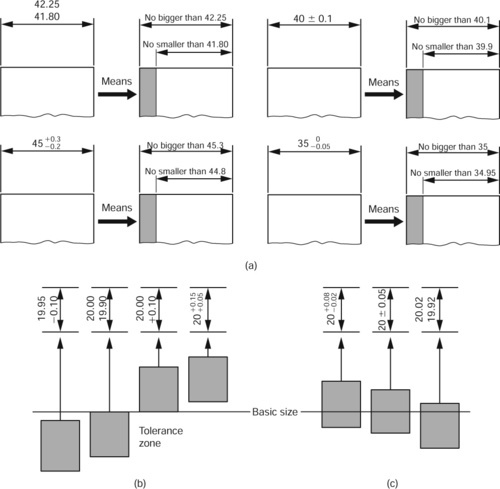
• Tolerance: This is the difference between the limits of size. That is, the upper limit minus the lower limit. Tolerances may be bilateral or unilateral as shown in Fig. 7.1(b) and (c).
• Deviation: This is the difference between the basic size and the limits. The deviation may be symmetrical, in which case the limits are equally spaced above and below the basic size (e.g. 50.00 ± 0.15 mm). Alternatively, the deviation may be asymmetrical, in which case the deviation may be greater on one side of the basic size than on the other (e.g. 50.00 + 0.25 or −0.05).
• Mean size: This size lies halfway between the upper and lower limits of size, and must not be confused with either the nominal size nor the basic size. It is only the same as the basic size when the deviation is symmetrical.
• Minimum clearance (allowance): This is the clearance between a shaft and a hole under maximum metal conditions. That is, the largest shaft in the smallest hole that the limits will allow. It is the tightest fit between shaft and hole that will function correctly. With a clearance fit the allowance is positive. With an interference fit the allowance is negative. These types of fit are discussed in the next section.
7.1.2 Classes of fit
Figure 7.2(a) shows the classes of fit that may be obtained between mating components. In the hole basis system the hole size is kept constant and the shaft size is varied to give the required class of fit. In an interference fit the shaft is always slightly larger than the hole. In a clearance fit the shaft is always slightly smaller than the hole. A transition fit occurs when the tolerances are so arranged that under maximum metal conditions (largest shaft: smallest hole) an interference fit is obtained, and that under minimum metal conditions (largest hole: smallest shaft) a clearance fit is obtained. The hole basis system is the most widely used since most holes are produced by using standard tools such as drills and reamers. It is then easier to vary the size of the shaft by turning or grinding to give the required class of fit.
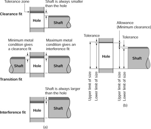
In a shaft basis system the shaft size is kept constant and the hole size is varied to give the required class of fit. Again, the classes of fit are interference fit transition fit and clearance fit. Figure 7.2(b) shows the terminology relating to limits and fits.
7.1.3 Accuracy
The greater the accuracy demanded by a designer, the narrower will be the tolerance band and the more difficult and costly will it be to manufacture the component within the limits specified. Therefore, for ease of manufacture at minimum cost, a designer never specifies an accuracy greater than is necessary to ensure the correct functioning of the component. The more important factors affecting accuracy when measuring components are as follows.
7.2 Standard systems of limits and fits (introduction)
This section is based on BS EN 20286-2: 1993 and is compatible with ISO 286-2: 1988 tables of standard tolerance grades and limit deviations for holes and shafts. These tables in these standards are suitable for all classes of work from the finest instruments to heavy engineering. It allows for the size of the work, the type of work, and provides for both hole basis and shaft basis systems as required.
7.2.1 Application of tables of limits and fits
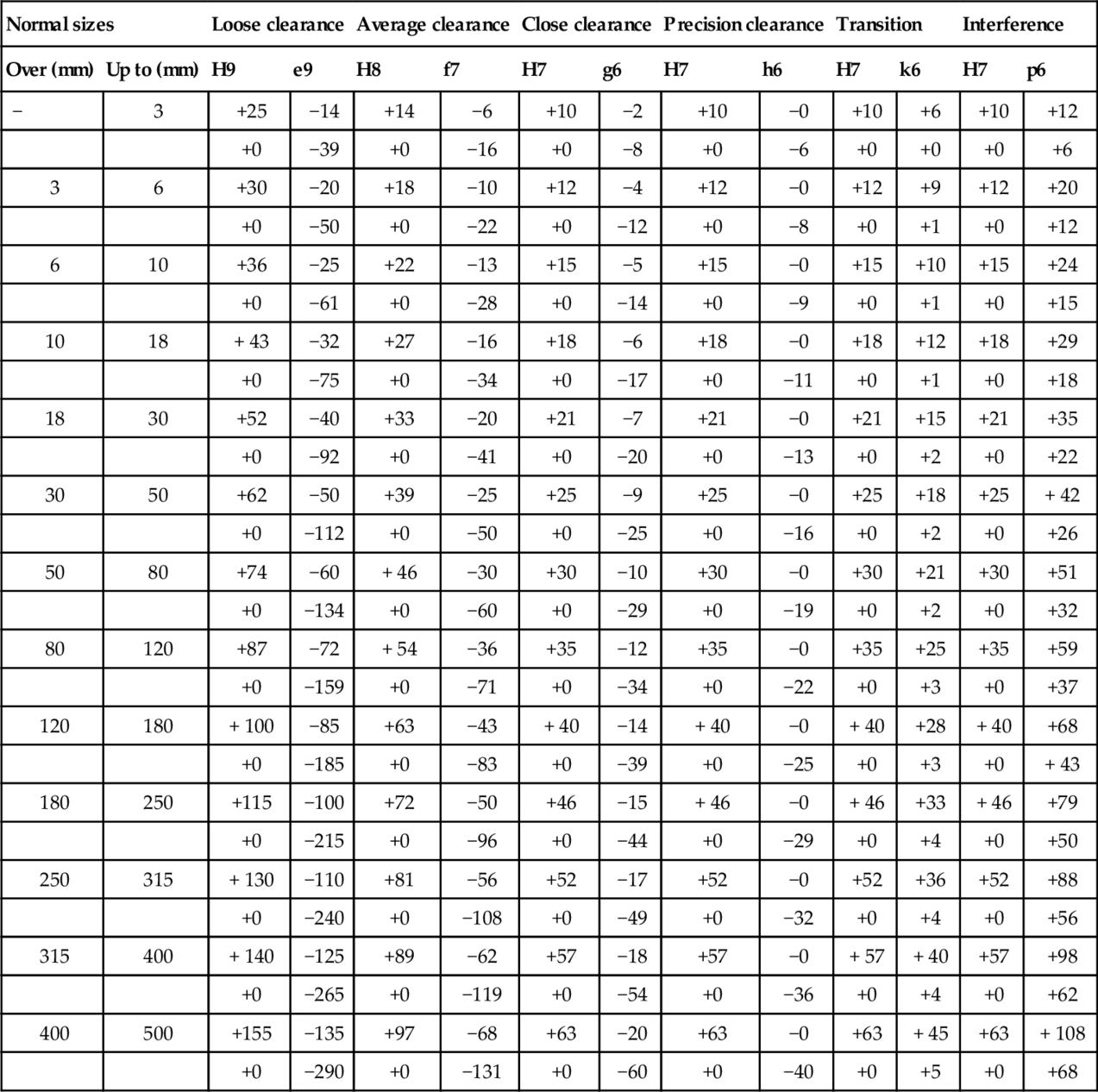
The tables provide for 28 types of shaft designated by lower-case letters, a, b, c, etc., and 28 types of hole designated by upper-case (capital) letters A, B, C, etc. To each type of shaft or hole the grade of tolerance is designated by a number 1–18 inclusive. The letter indicates the position of the tolerance relative to the basic size and is called the fundamental deviation. The number indicates the magnitude of the tolerance and is called the fundamental tolerance. A shaft is completely defined by its basic size, letter and number (e.g. 75 mm h6). Similarly a hole is completely defined by its basic size, letter and number, for example: 75 mm H7. Table 7.1 shows a selection of limits and fits for a wide range of hole and shaft combinations for a variety of applications.
Table 7.1
Primary selection of fits.
| Normal sizes | Loose clearance | Average clearance | Close clearance | Precision clearance | Transition | Interference | |||||||
| Over (mm) | Up to (mm) | H9 | e9 | H8 | f7 | H7 | g6 | H7 | h6 | H7 | k6 | H7 | p6 |
| − | 3 | +25 | −14 | +14 | −6 | +10 | −2 | +10 | −0 | +10 | +6 | +10 | +12 |
| +0 | −39 | +0 | −16 | +0 | −8 | +0 | −6 | +0 | +0 | +0 | +6 | ||
| 3 | 6 | +30 | −20 | +18 | −10 | +12 | −4 | +12 | −0 | +12 | +9 | +12 | +20 |
| +0 | −50 | +0 | −22 | +0 | −12 | +0 | −8 | +0 | +1 | +0 | +12 | ||
| 6 | 10 | +36 | −25 | +22 | −13 | +15 | −5 | +15 | −0 | +15 | +10 | +15 | +24 |
| +0 | −61 | +0 | −28 | +0 | −14 | +0 | −9 | +0 | +1 | +0 | +15 | ||
| 10 | 18 | + 43 | −32 | +27 | −16 | +18 | −6 | +18 | −0 | +18 | +12 | +18 | +29 |
| +0 | −75 | +0 | −34 | +0 | −17 | +0 | −11 | +0 | +1 | +0 | +18 | ||
| 18 | 30 | +52 | −40 | +33 | −20 | +21 | −7 | +21 | −0 | +21 | +15 | +21 | +35 |
| +0 | −92 | +0 | −41 | +0 | −20 | +0 | −13 | +0 | +2 | +0 | +22 | ||
| 30 | 50 | +62 | −50 | +39 | −25 | +25 | −9 | +25 | −0 | +25 | +18 | +25 | + 42 |
| +0 | −112 | +0 | −50 | +0 | −25 | +0 | −16 | +0 | +2 | +0 | +26 | ||
| 50 | 80 | +74 | −60 | + 46 | −30 | +30 | −10 | +30 | −0 | +30 | +21 | +30 | +51 |
| +0 | −134 | +0 | −60 | +0 | −29 | +0 | −19 | +0 | +2 | +0 | +32 | ||
| 80 | 120 | +87 | −72 | + 54 | −36 | +35 | −12 | +35 | −0 | +35 | +25 | +35 | +59 |
| +0 | −159 | +0 | −71 | +0 | −34 | +0 | −22 | +0 | +3 | +0 | +37 | ||
| 120 | 180 | + 100 | −85 | +63 | −43 | + 40 | −14 | + 40 | −0 | + 40 | +28 | + 40 | +68 |
| +0 | −185 | +0 | −83 | +0 | −39 | +0 | −25 | +0 | +3 | +0 | + 43 | ||
| 180 | 250 | +115 | −100 | +72 | −50 | +46 | −15 | + 46 | −0 | + 46 | +33 | + 46 | +79 |
| +0 | −215 | +0 | −96 | +0 | −44 | +0 | −29 | +0 | +4 | +0 | +50 | ||
| 250 | 315 | + 130 | −110 | +81 | −56 | +52 | −17 | +52 | −0 | +52 | +36 | +52 | +88 |
| +0 | −240 | +0 | −108 | +0 | −49 | +0 | −32 | +0 | +4 | +0 | +56 | ||
| 315 | 400 | + 140 | −125 | +89 | −62 | +57 | −18 | +57 | −0 | + 57 | + 40 | +57 | +98 |
| +0 | −265 | +0 | −119 | +0 | −54 | +0 | −36 | +0 | +4 | +0 | +62 | ||
| 400 | 500 | +155 | −135 | +97 | −68 | +63 | −20 | +63 | −0 | +63 | + 45 | +63 | + 108 |
| +0 | −290 | +0 | −131 | +0 | −60 | +0 | −40 | +0 | +5 | +0 | +68 | ||
source: Abstract from BS 4500 (data compatible with BS EN 20286-2: 1993).
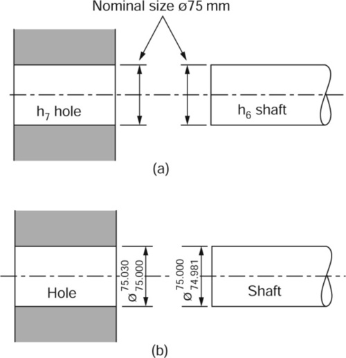
Consider a precision clearance fit as given by a 75 mm H7 hole and a 75 mm h6 shaft as shown in Fig. 7.3(a) This hole and shaft combination is high-lighted in Table 7.1
Hole
Enter the table along diameter band 50–80 mm, and where this band crosses the column H7 the limits are given as +30 and +0. These dimensions are in units of 0.001 mm [0.001 mm = 1 micrometre (µm)j. Therefore, when applied to a basic size of 75 mm, they give working limits of 75.030 and 75.000 mm as shown in Fig. 7.3(b)
shaft
Enter the table along diameter band 50–80 mm, and where this band crosses the column h6 the limits are given as −0 and −19. Again these dimensions are in units of 0.001 mm (1 µm). Therefore, when applied to a basic size of 75 mm, they give working limits of 75.000 and 74.981 mm as shown in Figure 7.3(b)
7.2.2 Selection of tolerance grades
From what has already been stated, it is obvious that the closer the limits (smaller the tolerance) the more difficult and expensive it is to manufacture a component. It is no use specifying very small (close) tolerances if the manufacturing process specified by the designer cannot achieve such a high degree of precision. Alternatively there is no point in choosing a process on grounds of low cost if it cannot achieve the accuracy necessary for the component to function correctly. Table 7.2 based on BS EN 20286–1: 1993 shows the standard tolerances from which the tables of limits and fits are derived.
Table 7.2
Numerical values of standard tolerance grades IT for basic sizes up to 3 150mm1
| Basic size mm | Standard tolerance grades | ||||||||||||||||||
| IT12 | IT22 | IT32 | IT42 | IT52 | IT6 | IT7 | IT8 | IT9 | IT10 | IT11 | IT12 | IT13 | IT143 | IT153 | IT163 | IT173 | IT183 | ||
| Above | Up to and including | Tolerances | |||||||||||||||||
| μm | mm | ||||||||||||||||||
| − | 33 | 0.8 | 1.2 | 2 | 3 | 4 | 6 | 10 | 14 | 25 | 40 | 60 | 0.1 | 0.14 | 0.25 | 0.4 | 0.6 | 1 | 1.4 |
| 3 | 6 | 1 | 1.5 | 2.5 | 4 | 5 | 8 | 12 | 18 | 30 | 48 | 75 | 0.12 | 0.18 | 0.3 | 0.48 | 0.75 | 1.2 | 1.8 |
| 6 | 10 | 1 | 1.5 | 2.5 | 4 | 6 | 9 | 15 | 22 | 36 | 58 | 90 | 0.15 | 0.22 | 0.36 | 0.58 | 0.9 | 1.5 | 2.2 |
| 10 | 18 | 1.2 | 2 | 3 | 5 | 8 | 11 | 18 | 27 | 43 | 70 | 110 | 0.18 | 0.27 | 0.43 | 0.7 | 1.1 | 1.8 | 2.7 |
| 18 | 30 | 1.5 | 2.5 | 4 | 6 | 9 | 13 | 21 | 33 | 52 | 84 | 130 | 0.21 | 0.33 | 0.52 | 0.84 | 1.3 | 2.1 | 3.3 |
| 30 | 50 | 1.5 | 2.5 | 4 | 7 | 11 | 16 | 25 | 39 | 62 | 100 | 160 | 0.25 | 0.39 | 0.62 | 1 | 1.6 | 2.5 | 3.9 |
| 50 | 80 | 2 | 3 | 5 | 8 | 13 | 19 | 30 | 46 | 74 | 120 | 190 | 0.3 | 0.46 | 0.74 | 1.2 | 1.9 | 3 | 4.6 |
| 80 | 120 | 2.5 | 4 | 6 | 10 | 15 | 22 | 35 | 54 | 87 | 140 | 220 | 0.35 | 0.54 | 0.87 | 1.4 | 2.2 | 3.5 | 5.4 |
| 120 | 180 | 3.5 | 5 | 8 | 12 | 18 | 25 | 40 | 63 | 100 | 160 | 250 | 0.4 | 0.63 | 1 | 1.6 | 2.5 | 4 | 6.3 |
| 180 | 250 | 4.5 | 7 | 10 | 14 | 20 | 29 | 46 | 72 | 115 | 185 | 290 | 0.46 | 0.72 | 1.15 | 1.85 | 2.9 | 4.6 | 7.2 |
| 250 | 315 | 6 | 8 | 12 | 16 | 23 | 32 | 52 | 81 | 130 | 210 | 320 | 0.52 | 0.81 | 1.3 | 2.1 | 3.2 | 5.2 | 8.1 |
| 315 | 400 | 7 | 9 | 13 | 18 | 25 | 36 | 57 | 89 | 140 | 230 | 360 | 0.57 | 0.89 | 1.4 | 2.3 | 3.6 | 5.7 | 8.9 |
| 400 | 500 | 8 | 10 | 15 | 20 | 27 | 40 | 63 | 97 | 155 | 250 | 400 | 0.63 | 0.97 | 1.55 | 2.5 | 4 | 6.3 | 9.7 |
| 500 | 6302 | 9 | 11 | 16 | 22 | 32 | 44 | 70 | 110 | 175 | 280 | 440 | 0.7 | 1.1 | 1.75 | 2.8 | 4.4 | 7 | 11 |
| 630 | 8002 | 10 | 13 | 18 | 25 | 36 | 50 | 80 | 125 | 200 | 320 | 500 | 0.8 | 1.25 | 2 | 3.2 | 5 | 8 | 12.5 |
| 800 | 10002 | 11 | 15 | 21 | 28 | 40 | 56 | 90 | 140 | 230 | 360 | 560 | 0.9 | 1.4 | 2.3 | 3.6 | 5.6 | 9 | 14 |
| 1000 | 12502 | 13 | 18 | 24 | 33 | 47 | 66 | 105 | 165 | 260 | 420 | 660 | 1.05 | 1.65 | 2.6 | 4.2 | 6.6 | 10.5 | 16.5 |
| 1250 | 16002 | 15 | 21 | 29 | 39 | 55 | 78 | 125 | 195 | 310 | 500 | 780 | 1.25 | 1.95 | 3.1 | 5 | 7.8 | 12.5 | 19.5 |
| 1600 | 20002 | 18 | 25 | 35 | 46 | 65 | 92 | 150 | 230 | 370 | 600 | 920 | 1.5 | 2.3 | 3.7 | 6 | 9.2 | 15 | 23 |
| 2000 | 25002 | 22 | 30 | 41 | 55 | 78 | 110 | 175 | 280 | 440 | 700 | 1100 | 1.75 | 2.8 | 4.4 | 7 | 11 | 17.5 | 28 |
| 2500 | 31502 | 26 | 36 | 50 | 68 | 96 | 135 | 210 | 330 | 540 | 860 | 1350 | 2.1 | 3.3 | 5.4 | 8.6 | 13.5 | 21 | 33 |
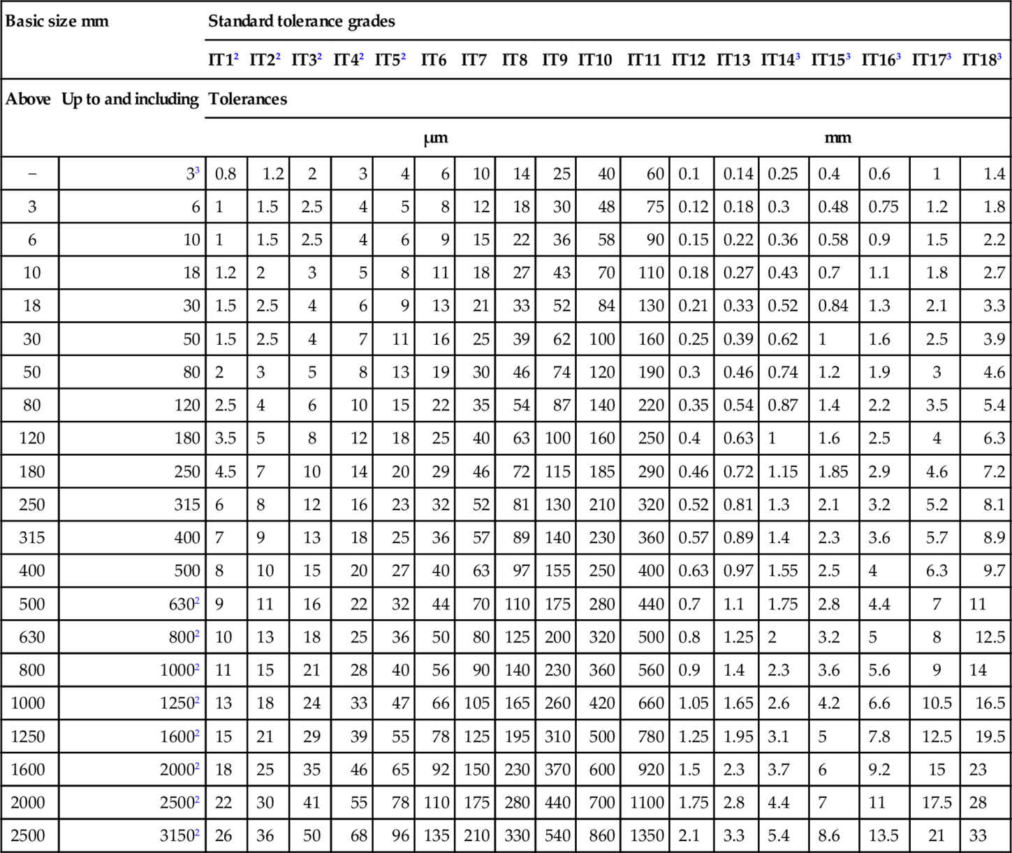
Note: This table, taken from ISO 286-1, has been included in this part of ISO 286 to facilitate understanding and use of the system.
1 Values for standard tolerance grades IT01 and IT0 for basic sizes less than or equal to 500 mm are given in ISO 286-1, Annex A, Table 5.
2 Values for standard tolerance grades IT1 to IT5 (inclusive) for basic sizes over 500 mm are included for experimental use.
3 Standard tolerance grades IT14 to IT18 (inclusive) shall not be used for basic sizes less than or equal to 1 mm.
It can be seen that as the International Tolerance (IT) number gets larger, so the tolerance increases. The recommended relationship between process and standard tolerance is as follows:
| IT16 | Sand casting, flame cutting (coarsest tolerance) |
| IT15 | Stamping |
| IT14 | Die-casting, plastic moulding |
| IT13 | Presswork, extrusion |
| IT12 | Light presswork, tube drawing |
| IT11 | Drilling, rough turning, boring |
| IT10 | Milling, slotting, planing, rolling |
| IT9 | Low grade capstan and automatic lathe work |
| IT8 | Centre lathe, capstan and automatic lathe work |
| IT7 | High-quality turning, broaching, honing |
| IT6 | Grinding, fine honing |
| IT5 | Machine lapping, fine grinding |
| IT4 | Gauge making, precision lapping |
| IT3 | High quality gap gauges |
| IT2 | High quality plug gauges |
| IT1 | Slip gauges, reference gauges (finest tolerance). |
7.1 Example
Determine a process that is suitable for manufacturing the shaft shown in Fig. 7.4
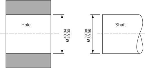
From Table 7.2 it can be seen that for a shaft of 40 mm nominal diameter and a tolerance of 0.03 mm (30 µm) the IT number lies between IT7 and IT8. Therefore a good turned finish would be sufficiently accurate. However to avoid wear the shaft would probably receive some form of heat treatment to harden the bearing surfaces, in which case the tolerance could easily be achieved by commercial quality cylindrical grinding.
7.3 Geometric tolerancing
Geometric tolerancing is a complex subject and there is only room to consider the basic principles in this volume. The reader is referred to BS ISO 1101: 2004 for a detailed explanation and examples of applications. The linear tolerancing of component dimensions is only concerned with the limits of size within which the component must be manufactured. Geometric tolerancing takes the dimensioning of components further and is concerned with the correct geometric shape of the component.
The importance of correct geometric accuracy as well as correct dimensional accuracy is being increasingly recognized.
Figure 7.5(a) shows a shaft whose dimensions have been given limits of size. The difference between the given limits is called the tolerance. For many applications, if the process used can achieve the dimensional tolerance, it will also produce a geometrically correct form. For example, the shaft shown in Fig. 7.5(a) would most likely be cylindrically ground to achieve the dimensional accuracy specified. Cylindrical grinding between centres should give a satisfactory degree of roundness. However, the shaft could also be mass-produced by centreless grinding and some out-of-roundness may occur such as ovality and lobing. Figure 7.5(b) shows how the shaft can be out-of-round yet still remain within its limits of size.

If cylindricity is important for the correct functioning of the component, then additional information must be added to the drawing to emphasize this point. This additional informa-tion is a geometrical tolerance which, in this case, would be added as shown in Fig. 7.6(a)

The symbol in the box indicates cylindricity, and the number indicates the geometrical tolerance. Figure 7.6(b) shows the interpretation of this tolerance.
7.3.1 Geometrical tolerance (principles)
In some circumstances, dimensions and tolerance of size, however well applied, do not impose the necessary control of form. If control of form is necessary then geometrical tolerances must be added to the component drawing. Geometrical tolerances should be specified for all requirements critical to the interchangeability and correct functioning of components. An exception can be made when the machinery and techniques used can be relied upon to achieve the required standard of form. Geometrical tolerances may also need to be specified even when no special size tolerance is given. For example, the thickness of a surface plate is of little importance, but its accuracy of flatness is of fundamental importance.
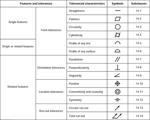
Figure 7.7 shows the standard tolerance symbols as specified in BS ISO 1101: 1983 and it can be seen that they are arranged into groups according to their function. In order to apply geometrical tolerances it is first necessary to consider the following definitions.
7.3.2 Tolerance frame
The tolerance frame is a rectangular frame (box) that is divided into two or more compartments containing the requisite information. Reading from left to right, this information is as shown in Fig. 7.8(a) and includes:
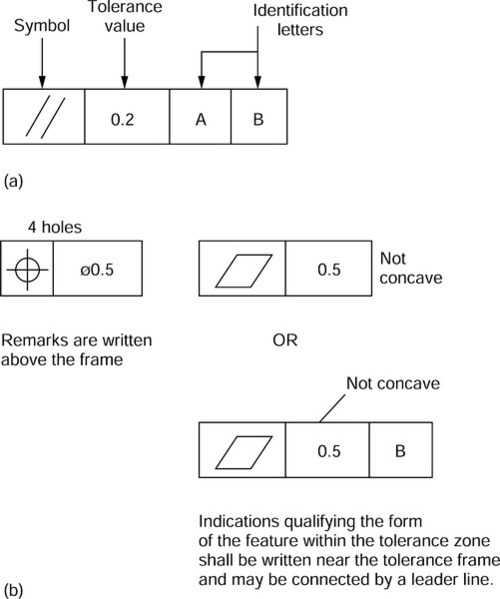
• The tolerance value in the same units as the associated linear dimension.
• If required, a letter or letters identifying the datum feature or features.
• If required, additional remarks may be added as shown in Fig. 7.8(b)
7.3.3 Geometrical tolerance
This is the maximum permissible overall variation of form or of position of a feature. That is, it defines the size and shape of a tolerance zone within which the surface, median plane or axis of the feature is to lie. It represents the full indicator movement it causes where testing with a dial test indicator (DTI) is applicable, for example, the ‘run-out’ of a shaft rotated about its own axis.
7.3.4 Tolerance zone
This is the zone within which the feature has to be contained. Thus, according to the characteristic that is to be toleranced and the manner in which it is to be dimensioned, the tolerance zone is one of the following:
• The area between two parallel lines or two parallel straight lines.
• The space between two parallel surfaces or two parallel planes.
• The space within a parallelepiped.
Note
The tolerance zone, once established, permits any feature to vary within that zone. If it is considered necessary to prohibit sudden changes in surface direction, or to control the rate of change of a surface within this zone, this should be additionally specified.
7.3.5 Geometrical reference frame
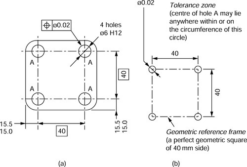
This is the diagram composed of the constructional dimensions that serve to establish the true geometrical relationships between positional features in any one group as shown in Fig. 7.9 For example, the symbol indicates that the hole centre may lie anywhere within a circle of 0.02 mm diameter that is itself centred upon the intersection of the frame. The dimension indicates that the reference frame is a geometrically perfect square of side length 40 mm.
7.3.6 Applications of geometrical tolerances
Figure 7.9 shows a plate in which four holes need to be drilled. For ease of assembly, the relationship between the hole-centres is more important than the group position on the plate. Therefore a combination of dimensional and geometrical tolerances has to be used.
Using the dimensional tolerances and the boxed dimension that defines true position, it is possible to determine the pattern locating tolerance zone for each of the holes as shown in Fig. 7.10. That is, the reference frame (which must always by a perfect square of side length 40 mm in this example) may lie in any position providing its corners are within the shaded boxes. The shaded boxes represent the dimensional tolerance. The hole centres may then (in this example) lie anywhere within the 0.02 mm circles that are themselves centred upon the corners of the reference frame.
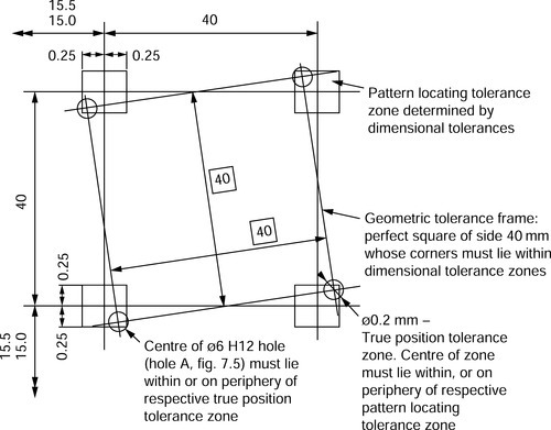
Figure 7.11 shows a stepped shaft with four concentric diameters and a flange that must run true with the datum axis. The shaft is to be located within journals at X and Y, and these are identified as datums. Note the use of leader lines terminating in solid triangles resting upon the features to be used as datums. The common axis of these datum diameters is used as a datum axis for relating the tolerances controlling the concentricity of the remaining diameters and the true running of the flange face. Figure 7.11(a) also shows that the dependent diameters and face carry geometric tolerances as well as dimensional tolerances. The tolerance frames carry the concentricity symbol, the concentricity toler-ance and the datum identification letters. These identification letters show that the concentricity of the remaining diameters is relative to the common axis of the datum diameters X and Y. The tolerance frame whose leader touches the flange face indicates that this face must run true, within the tolerance indicated when the shaft rotates in the vee-blocks supporting it at X and Y, as shown in Fig. 7.11(b)

These two examples are in no way a comprehensive resume of the application of geometric tolerancing but stand as an introduction to the subject and as an introduction to BS ISO 1101:1983. This British Standard details the full range of applications and their interpretation, and includes a number of fully dimensioned examples.
7.4 Virtual size
To understand this section, it is necessary to introduce the terms maximum metal condition and minimum metal condition.
• The maximum metal condition exists for both the hole and the shaft when the least amount of metal has been removed but the component is still within its specified limits of size, that is, the largest shaft and smallest hole that will lie within the specified tolerance.
• The minimum metal condition exists when the greatest amount of metal has been removed but the component is still within its limits of size, that is the largest hole and the smallest shaft that will lie within the specified tolerance.
Figure 7.12 shows the effect of a change in geometry on the fit of a pin in a hole. In Figure 7.12(a), an ideal pin is used with a straight axis. It can be seen that, as drawn, there is clearance between the pin and the hole. However, in Fig. 7.12(b) the pin is distorted and now becomes a tight fit in the hole despite the fact that its dimensional tolerance has not changed.

Figure 7.13(a) shows the same pin and hole, only this time dimensional and geometrical tolerances have been added to the pin. For simplicity the hole is assumed to be geometrically correct. The tolerance frame shows a straightness tolerance of 0.05 mm. This means that the axis of the pin can bow within the confines of an imaginary cylinder 0.05 mm diameter. The dimensional limits indicate a tolerance of 0.08 mm. The worst conditions for assembly (tightest fit) occurs when the pin and the hole are in their respective maximum metal conditions and, in addition, the maximum error permitted by the geometrical tolerancing is also present. Figure 7.13(b) shows the fit between the pin and the hole under these conditions.
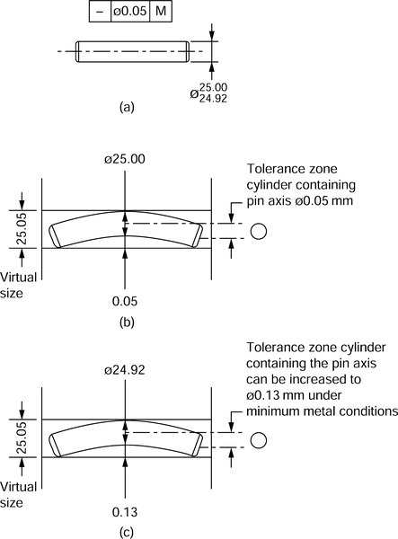
Under such conditions the pin will just enter a truly straight and cylindrical hole equal to the pin diameter under maximum metal conditions (25.00 mm) plus the geometrical tolerance of 0.05 mm, that is a hole diameter of 25.05 mm. This theoretical hole diameter of 25.05 mm is referred to as the virtual size for the pin.
Under minimum metal conditions, the geometrical tolerance for the pin can be increased without altering the fit of the pin in the hole. As shown in Fig. 7.13(c), the geometric tolerance can now be increased to 0.13 mm without any increase in the virtual size or the change of fit.
7.5 The economics of geometrical tolerancing
Figure 7.14 shows a typical relationship between tolerance and manufacturing costs for any given manufactured component part. As tolerance is reduced the manufacturing costs tend to rise rapidly. The addition of geometrical tolerances on top of the dimensional tolerances aggravates this situation still further. Thus geometric tolerances are only applied if the function and the interchangeability of the component is critical and absolutely dependent upon a tightly controlled geometry. To keep costs down, it can often be assumed that the machine or process will provide adequate geometric control and only dimensional tolerances are added to the component drawing. For example, it can generally be assumed that a component finished on a cylindrical grinding machine between centres will be straight and cylindrical to a high degree of geometrical accuracy. However, current trends in quality control and just-in-time (JIT) scheduling tends to increase the demand for closer dimensional and geometrical control to ensure no hold ups occur during assembly and that any quality specifications are met first time without the need for corrective action or rejection by the customer.
