
Engineering Mathematics
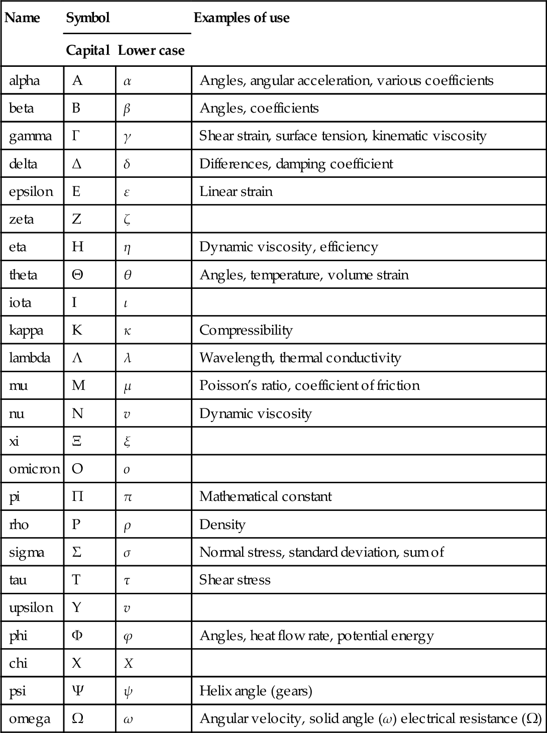
1.1 The Greek alphabet
| Name | Symbol | Examples of use | |
| Capital | Lower case | ||
| alpha | A | α | Angles, angular acceleration, various coefficients |
| beta | B | β | Angles, coefficients |
| gamma | Γ | γ | Shear strain, surface tension, kinematic viscosity |
| delta | Δ | δ | Differences, damping coefficient |
| epsilon | E | ε | Linear strain |
| zeta | Z | ζ | |
| eta | H | η | Dynamic viscosity, efficiency |
| theta | Θ | θ | Angles, temperature, volume strain |
| iota | I | ι | |
| kappa | K | κ | Compressibility |
| lambda | Λ | λ | Wavelength, thermal conductivity |
| mu | M | μ | Poisson’s ratio, coefficient of friction |
| nu | N | v | Dynamic viscosity |
| xi | Ξ | ξ | |
| omicron | O | ο | |
| pi | Π | π | Mathematical constant |
| rho | P | ρ | Density |
| sigma | Σ | σ | Normal stress, standard deviation, sum of |
| tau | T | τ | Shear stress |
| upsilon | Y | v | |
| phi | ϕ | ϕ | Angles, heat flow rate, potential energy |
| chi | X | X | |
| psi | Ψ | ψ | Helix angle (gears) |
| omega | Ω | ω | Angular velocity, solid angle (ω) electrical resistance (Ω) |
1.2 Mathematical symbols
| Is equal to | = |
| Is identically equal to | ≡ |
| Approaches | → |
| Is smaller than | < |
| Is smaller than or equal to | ≤ |
| Magnitude of a | |a| |
| Square root of a | √a |
| Mean value of a | ˉa |
| Sum | ∑ |
| Complex operator | i, j |
| Imaginary part of z | Im z |
| Argument of z | arg z |
| Is not equal to | ≠ |
| Is approximately equal to | ≈ |
| Is proportional to | ∝ |
| Is larger than | > |
| Is larger than or equal to | ≥ |
| a raised to power n | an |
| nth root of a | n√a |
| Factorial a | a! |
| Product | ∏ |
| Real part of z | Re z |
| Modulus of z | |z| |
| Complex conjugate of z | z* |
| a multiplied by b | ab, a•b,a×b |
| a divided by b | a/b,ab,ab−1 |
| Function of x | f(x) |
| Variation of x | δx |
| Finite increment of x | Δx |
| Limit to which f(x) tends as x approaches a | limx→af(X) |
| Differential coefficient of f(x) with respect to x | dfdx,df/dx,f′(x) |
| Indefinite integral of f(x) with respect to x | ∫f(x)dx |
| Increase in value of f(x) as x increases from a to b | [f(x)]ba |
| Definite integral of f(x) from x = a to x = b | ∫baf(x)dx |
| Logarithm to the base 10 of x | lgX,log10X |
| Logarithm to the base a of x | logaX |
| Exponential of x | exp x, eX |
| Natural logarithm | In x, logex |
| Inverse sine of x | arcsinx |
| Inverse cosine of x | arccosx |
| Inverse tangent of x | arctanx |
| Inverse secant of x | arcsecx |
| Inverse cosecant of x | arccosecx |
| Inverse cotangent of x | arccotx |
| Inverse hyperbolic sine of x | arcsinhx |
| Inverse hyperbolic cosine of x | arcoshx |
| Inverse hyperbolic tangent of x | artanhx |
| Inverse hyperbolic cosecant of x | arcosechx |
| Inverse hyperbolic secant of x | arsechx |
| Inverse hyperbolic cotangent of x | arcothx |
| Vector | A |
| Magnitude of vector A | |A|,A |
| Scalar products of vectors A and B | A•B |
| Vector products of vectors A and B | A×B,A∧B |
1.3 Units: SI
1.3.1 Basic and supplementary units
The International System of Units (SI) is based on nine physical quantities.
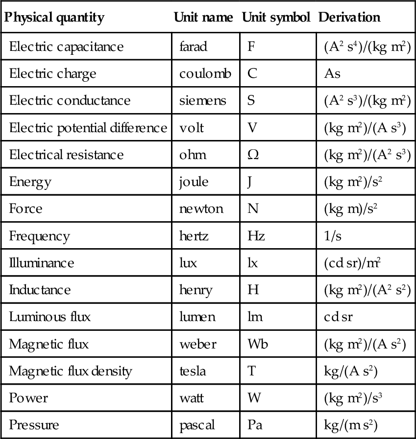
1.3.2 Derived units
By dimensionally appropriate multiplication and/or division of the units shown above, derived units are obtained. Some of these are given special names.
| Physical quantity | Unit name | Unit symbol | Derivation |
| Electric capacitance | farad | F | (A2 s4)/(kg m2) |
| Electric charge | coulomb | C | As |
| Electric conductance | siemens | S | (A2 s3)/(kg m2) |
| Electric potential difference | volt | V | (kg m2)/(A s3) |
| Electrical resistance | ohm | Ω | (kg m2)/(A2 s3) |
| Energy | joule | J | (kg m2)/s2 |
| Force | newton | N | (kg m)/s2 |
| Frequency | hertz | Hz | 1/s |
| Illuminance | lux | lx | (cd sr)/m2 |
| Inductance | henry | H | (kg m2)/(A2 s2) |
| Luminous flux | lumen | lm | cd sr |
| Magnetic flux | weber | Wb | (kg m2)/(A s2) |
| Magnetic flux density | tesla | T | kg/(A s2) |
| Power | watt | W | (kg m2)/s3 |
| Pressure | pascal | Pa | kg/(m s2) |
Some other derived units not having special names.
| Physical quantity | Unit | Unit symbol |
| Acceleration | metre per second squared | m/s2 |
| Angular velocity | radian per second | rad/s |
| Area | square metre | m2 |
| Current density | ampere per square metre | A/m2 |
| Density | kilogram per cubic metre | kg/m3 |
| Dynamic viscosity | pascal second | Pa s |
| Electric charge density | coulomb per cubic metre | C/m3 |
| Electric field strength | volt per metre | V/m |
| Energy density | joule per cubic metre | J/m3 |
| Heat capacity | joule per kelvin | J/K |
| Heat flux density | watt per square metre | W/m2 |
| Kinematic viscosity | square metre per second | m2/s |
| Luminance | candela per square metre | cd/m2 |
| Magnetic field strength | ampere per metre | A/m |
| Moment of force | newton metre | N m |
| Permeability | henry per metre | H/m |
| Permittivity | farad per metre | F/m |
| Specific volume | cubic metre per kilogram | m3/kg |
| Surface tension | newton per metre | N/m |
| Thermal conductivity | watt per metre kelvin | W/(m K) |
| Velocity | metre per second | m/s |
| Volume | cubic metre | m3 |
1.3.3 Units: not SI
Some of the units which are not part of the SI system, but which are recognized for continued use with the SI system, are as shown.
| Physical quantity | Unit name | Unit symbol | Definition |
| Angle | degree | ° | (π/180) rad |
| Angle | minute | ' | (π/10800) rad |
| Angle | second | " | (π/648000) rad |
| Celsius temperature | degree Celsius | °C | K – 273.2 (For K see 1.3.1) |
| Dynamic viscosity | poise | P | 10−1 Pas |
| Energy | calorie | cal | ≈4.18J(π/180)rad |
| Fahrenheit temperature | degree Fahrenheit | °F | (95)∘C+32 |
| Force | kilogram force | kgf | ≈9.807 N |
| Kinematic viscosity | stokes | St | 10–4m2/s |
| Length | inch | in. | 2.54 Χ 10−2m |
| Length | micron | µm | 10−6m |
| Mass | pound | lb | ≈0.454kg |
| Mass | tonne | t | 103kg |
| Pressure | atmosphere | atm | 101 325 Pa |
| Pressure | bar | bar | 105 Pa |
| Pressure | millimetre of mercury | mm Hg | ≈ 133.322 Pa |
| Pressure | torr | torr | ≈ 133.322 Pa |
| Thermodynamic temperature | degree Rankine | °R | °F + 459.7 |
| Time | minute | min | 60 s |
| Time | hour | h | 3600s |
| Time | day | d | 86400s |

1.3.4 Notes on writing symbols
(a) Symbols should be in roman type lettering: thus cm, not cm.
(b) Symbols should remain unaltered in the plural: thus cm, not cms.
(c) There should be a space between the product of two symbols: thus N m, not Nm.
(d) Index notation may be used: thus m/s may be written as m s−1 and W/(m K) as Wm−1 K−1
1.3.5 Decimal multiples of units
For quantities which are much larger or much smaller than the units so far given, decimal multiples of units are used.
Internationally agreed multiples are as shown.
For small quantities
For large quantities
Notes
(a) A prefix is used with the gram, not the kilogram: thus Mg, not kkg.
(b) A prefix may be used for one or more of the unit symbols: thus kN m, N mm and kN mm are all acceptable.
(c) Compound prefixes should not be used: thus ns, not mµs.
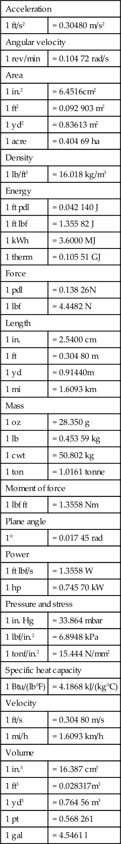
1.4 Conversion factors for units
The conversion factors shown below are accurate to five significant figures where FPS is the foot-pound-second system.
1.4.1 FPS to SI units
| Acceleration | |
| 1 ft/s2 | = 0.30480 m/s2 |
| Angular velocity | |
| 1 rev/min | = 0.104 72 rad/s |
| Area | |
| 1 in.2 | = 6.4516cm2 |
| 1 ft2 | = 0.092 903 m2 |
| 1 yd2 | = 0.83613 m2 |
| 1 acre | = 0.404 69 ha |
| Density | |
| 1 lb/ft3 | = 16.018 kg/m3 |
| Energy | |
| 1 ft pdl | = 0.042 140 J |
| 1 ft lbf | = 1.355 82 J |
| 1 kWh | = 3.6000 MJ |
| 1 therm | = 0.105 51 GJ |
| Force | |
| 1 pdl | = 0.138 26N |
| 1 lbf | = 4.4482 N |
| Length | |
| 1 in. | = 2.5400 cm |
| 1 ft | = 0.304 80 m |
| 1 yd | = 0.91440m |
| 1 mi | = 1.6093 km |
| Mass | |
| 1 oz | = 28.350 g |
| 1 lb | = 0.453 59 kg |
| 1 cwt | = 50.802 kg |
| 1 ton | = 1.0161 tonne |
| Moment of force | |
| 1 lbf ft | = 1.3558 Nm |
| Plane angle | |
| 1° | = 0.017 45 rad |
| Power | |
| 1 ft lbf/s | = 1.3558 W |
| 1 hp | = 0.745 70 kW |
| Pressure and stress | |
| 1 in. Hg | = 33.864 mbar |
| 1 lbf/in.2 | = 6.8948 kPa |
| 1 tonf/in.2 | = 15.444 N/mm2 |
| Specific heat capacity | |
| 1 Btu/(lb°F) | = 4.1868 kJ/(kg°C) |
| Velocity | |
| 1 ft/s | = 0.304 80 m/s |
| 1 mi/h | = 1.6093 km/h |
| Volume | |
| 1 in.3 | = 16.387 cm3 |
| 1 ft3 | = 0.028317m3 |
| 1 yd3 | = 0.764 56 m3 |
| 1 pt | = 0.568 261 |
| 1 gal | = 4.5461 l |
1.4.2 SI to FPS units
| Acceleration | |
| 1 m/s2 | = 3.2808 ft/s2 |
| Angular velocity | |
| 1 rad/s | = 9.5493 rev/min |
| Area | |
| 1 cm2 | = 0.155 00 in.2 |
| 1m2 | = 10.764 ft2 |
| 1m2 | = 1.1960yd2 |
| 1 ha | = 2.4711 acre |
| Density | |
| 1 kg/m3 | = 0.062 428 lb/ft3 |
| Energy | |
| 1J | = 23.730 ft pdl |
| 1J | = 0.737 56ft lbf |
| 1 MJ | = 0.277 78 kWh |
| 1 GJ | = 9.4781 therm |
| Force | |
| 1N | = 7.2330 pdl |
| 1N | = 0.22481 lbf |
| Length | |
| 1 cm | = 0.393 70 in. |
| 1 m | = 3.2808ft |
| 1 m | = 1.0936 yd |
| 1 km | = 0.621 37 mi |
| Mass | |
| 1g | = 0.035 274oz |
| 1 kg | = 2.2046 lb |
| 1 kg | = 2.2046 lb |
| 1 tonne | = 0.984 21 ton |
| Moment of force | |
| 1 Nm | = 0.737 56 lbf ft |
| Plane angle | |
| 1 rad | = 57.296° |
| Power | |
| 1W | = 0.737 56ft lbf/s |
| 1 kW | = 1.3410 hp |
| Pressure and stress | |
| 1 mbar | = 0.029 53 in. Hg |
| 1 kPa | = 0.145 04 lbf/in.2 |
| 1 N/mm2 | = 0.064 749tonf/in.2 |
| Specific heat capacity | |
| 1 kJ/(kg °C) | = 0.23885 Btu/(lb°F) |
| Velocity | |
| 1 m/s | = 3.2808 ft/s |
| km/h | = 0.621 37 mi/h |
| Volume | |
| 1cm3 | = 0.061 024 in.3 |
| 1m3 | = 35.315ft3 |
| 1m3 | = 1.3080yd3 |
| 1l | = 1.7598 pt |
| 1l | = 0.21997 gal |

1.5 Preferred numbers
When one is buying, say, an electric lamp for use in the home, the normal range of lamps available is 15, 25, 40, 60, 100W and so on. These watt values approximately follow a geometric progression, roughly giving a uniform percentage change in light emission between consecutive sizes. In general, the relationship between the sizes of a commodity is not random but based on a system of preferred numbers.
Preferred numbers are based on R numbers devised by Colonel Charles Renard. The principal series used are R5, R10, R20, R40 and R80, and subsets of these series. The values within a series are approximate geometric progressions based on common ratios of 5√10,10√10,20√10,40√10and80√10,![]() representing changes between various sizes within a series of 58% for the R5 series, 26% for the R10, 12% for the R20, 6% for the R40 and 3% for the R80 series.
representing changes between various sizes within a series of 58% for the R5 series, 26% for the R10, 12% for the R20, 6% for the R40 and 3% for the R80 series.
Further details on the values and use of preferred numbers may be found in BS 2045:1965. The rounded values for the R5 series are given as 1.00, 1.60, 2.50, 4.00, 6.30 and 10.00; these values indicate that the electric lamp sizes given above are based on the R5 series. Many of the standards in use are based on series of preferred numbers and these include such standards as sheet and wire gauges, nut and bolt sizes, standard currents (A) and rotating speeds of machine tool spindles.
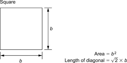
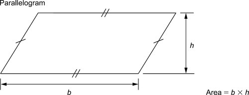
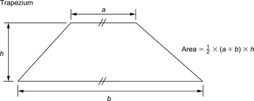
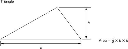
1.6 Mensuration
1.6.1 Plane figures
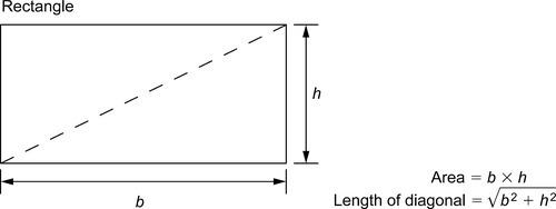
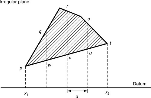
Several methods are used to find the shaded area, such as the mid-ordinate rule, the trapezoidal rule and Simpson’s rule. As an example of these, Simpson’s rule is as shown. Divide x1x2 into an even number of equal parts of width d. Let p, q, r, … be the lengths of vertical lines measured from some datum, and let A be the approximate area of the irregular plane, shown shaded. Then:
A=d3[(p+t)+4(q+s)+2r]−d3[(p+t)+4(u+w)+2r]
![]()
In general, the statement of Simpson’s rule is:
Approximate area=(d/3)×[(first+last)+4(sum of evens)+2(sum of odds)]
![]()
where first, last, evens, odds refer to ordinate lengths and d is the width of the equal parts of the datum line.
1.6.2 Solid objects
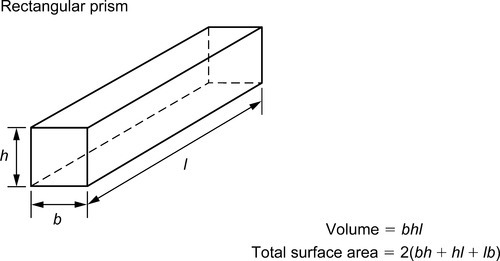

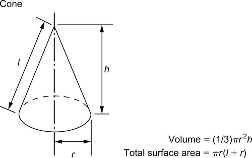
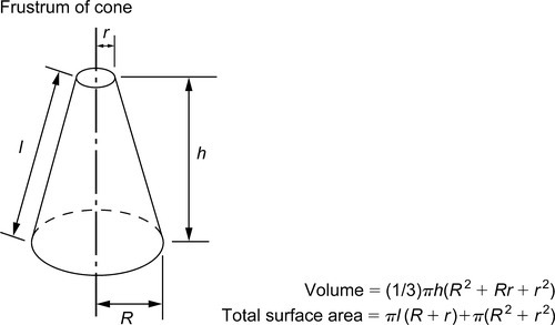
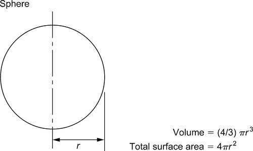
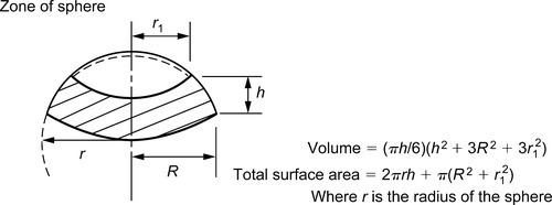

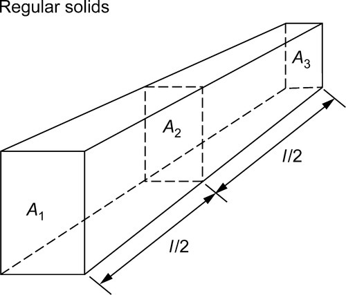
The volume of any regular solid can be found by using the prismoidal rule. Three parallel planes of areas A1, A3 and A2 are considered to be at the ends and at the centre of the solid, respectively. Then:
Volume=(l/6)(A1+4A2+A3)
![]()
Where:
l is the length of the solid.

Various methods can be used to determine volumes of irregular solids; one of these is by applying the principles of Simpson’s rule (see earlier this section). The solid is considered to be divided into an even number of sections by equally spaced, parallel planes, distance d apart and having areas of A1, A2, A3, …. Assuming, say, seven such planes, then approximate volume =(d/3)[(A1+A7)+4(A2+A4+A6)+2(A3+A5)].![]()
1.7 Powers, roots and reciprocals
| n | n2 | √n | √10n | n3 | (n)1/3 | (10n)1/3 | (100n)1/3 | 1/n |
| 1 | 1 | 1.000 | 3.162 | 1 | 1.000 | 2.154 | 4.642 | 1.000 00 |
| 2 | 4 | 1.414 | 4.472 | 8 | 1.260 | 2.714 | 5.848 | 0.500 00 |
| 3 | 9 | 1.732 | 5.477 | 27 | 1.442 | 3.107 | 6.694 | 0.333 33 |
| 4 | 16 | 2.000 | 6.325 | 64 | 1.587 | 3.420 | 7.368 | 0.250 00 |
| 5 | 25 | 2.236 | 7.071 | 125 | 1.710 | 3.684 | 7.937 | 0.200 00 |
| 6 | 36 | 2.449 | 7.746 | 216 | 1.817 | 3.915 | 8.434 | 0.166 67 |
| 7 | 49 | 2.646 | 8.367 | 343 | 1.913 | 4.121 | 8.879 | 0.142 86 |
| 8 | 64 | 2.828 | 8.944 | 512 | 2.000 | 4.309 | 9.283 | 0.125 00 |
| 9 | 81 | 3.000 | 9.487 | 729 | 2.080 | 4.481 | 9.655 | 0.111 11 |
| 10 | 100 | 3.162 | 10.000 | 1 000 | 2.154 | 4.642 | 10.000 | 0.100 00 |
| 11 | 121 | 3.317 | 10.488 | 1 331 | 2.224 | 4.791 | 10.323 | 0.090 91 |
| 12 | 144 | 3.464 | 10.954 | 1 738 | 2.289 | 4.932 | 10.627 | 0.08333 |
| 13 | 169 | 3.606 | 11.402 | 2 197 | 2.351 | 5.066 | 10.914 | 0.076 92 |
| 14 | 196 | 3.742 | 11.832 | 2 744 | 2.410 | 5.192 | 11.187 | 0.071 43 |
| 15 | 225 | 3.873 | 12.247 | 3375 | 2.466 | 5.313 | 11.447 | 0.066 67 |
| 16 | 256 | 4.000 | 12.649 | 4096 | 2.520 | 5.429 | 11.696 | 0.062 50 |
| 17 | 289 | 4.123 | 13.038 | 4913 | 2.571 | 5.540 | 11.935 | 0.058 82 |
| 18 | 324 | 4.243 | 13.416 | 5 832 | 2.621 | 5.646 | 12.164 | 0.055 56 |
| 19 | 361 | 4.359 | 13.784 | 6859 | 2.668 | 5.749 | 12.386 | 0.052 63 |
| 20 | 400 | 4.472 | 14.142 | 8 000 | 2.714 | 5.848 | 12.599 | 0.050 00 |
| 21 | 441 | 4.583 | 14.491 | 9 261 | 2.759 | 5.944 | 12.806 | 0.047 62 |
| 22 | 484 | 4.690 | 14.832 | 10 648 | 2.802 | 6.037 | 13.006 | 0.045 45 |
| 23 | 529 | 4.796 | 15.166 | 12 167 | 2.844 | 6.127 | 13.200 | 0.043 48 |
| 24 | 576 | 4.899 | 15.492 | 13 824 | 2.884 | 6.214 | 13.389 | 0.041 67 |
| 25 | 625 | 5.000 | 15.811 | 15 625 | 2.924 | 6.300 | 13.572 | 0.040 00 |
| 26 | 676 | 5.099 | 16.125 | 17 576 | 2.962 | 6.383 | 13.751 | 0.038 46 |
| 27 | 729 | 5.196 | 16.432 | 19 683 | 3.000 | 6.463 | 13.925 | 0.037 04 |
| 28 | 784 | 5.292 | 16.733 | 21 952 | 3.037 | 6.542 | 14.095 | 0.035 71 |
| 29 | 841 | 5.385 | 17.029 | 24389 | 3.072 | 6.619 | 14.260 | 0.034 48 |
| 30 | 900 | 5.477 | 17.321 | 27 000 | 3.107 | 6.694 | 14.422 | 0.033 33 |
| 31 | 961 | 5.568 | 17.607 | 29791 | 3.141 | 6.768 | 14.581 | 0.032 26 |
| 32 | 1024 | 5.657 | 17.889 | 32 768 | 3.175 | 6.840 | 14.736 | 0.031 25 |
| 33 | 1089 | 5.745 | 18.166 | 35 937 | 3.208 | 6.910 | 14.888 | 0.030 30 |
| 34 | 1156 | 5.831 | 18.439 | 39 304 | 3.240 | 6.980 | 15.037 | 0.029 41 |
| 35 | 1225 | 5.916 | 18.708 | 42 875 | 3.271 | 7.047 | 15.183 | 0.028 57 |
| 36 | 1296 | 6.000 | 18.974 | 46 656 | 3.302 | 7.114 | 15.326 | 0.027 78 |
| 37 | 1369 | 6.083 | 19.235 | 50 653 | 3.332 | 7.179 | 15.467 | 0.027 03 |
| 38 | 1444 | 6.164 | 19.494 | 54 872 | 3.362 | 7.243 | 15.605 | 0.026 32 |
| 39 | 1521 | 6.245 | 19.748 | 59 319 | 3.391 | 7.306 | 15.741 | 0.025 64 |
| 40 | 1600 | 6.325 | 20.000 | 64 000 | 3.420 | 7.368 | 15.874 | 0.025 00 |
| 41 | 1681 | 6.430 | 20.248 | 68 921 | 3.448 | 7.429 | 16.005 | 0.024 39 |
| 42 | 1764 | 6.481 | 20.494 | 74 088 | 3.476 | 7.489 | 16.134 | 0.023 81 |
| 43 | 1849 | 6.557 | 20.736 | 79 507 | 3.503 | 7.548 | 16.261 | 0.023 26 |
| 44 | 1936 | 6.633 | 20.976 | 85 184 | 3.530 | 7.606 | 16.386 | 0.022 73 |
| 45 | 2025 | 6.708 | 21.213 | 91 125 | 3.557 | 7.663 | 16.510 | 0.022 22 |
| 46 | 2116 | 6.782 | 21.448 | 97 336 | 3.583 | 7.719 | 16.631 | 0.021 74 |
| 47 | 2209 | 6.856 | 21.679 | 103 823 | 3.609 | 7.775 | 16.751 | 0.021 28 |
| 48 | 2304 | 6.928 | 21.909 | 110 592 | 3.634 | 7.830 | 16.869 | 0.020 83 |
| 49 | 2401 | 7.000 | 22.136 | 117 649 | 3.659 | 7.884 | 16.985 | 0.020 41 |
| 50 | 2500 | 7.071 | 22.361 | 125 000 | 3.684 | 7.937 | 17.100 | 0.020 00 |
| 51 | 2601 | 7.141 | 22.583 | 132 651 | 3.708 | 7.990 | 17.213 | 0.019 61 |
| 52 | 2704 | 7.211 | 22.804 | 140 608 | 3.733 | 8.041 | 17.325 | 0.019 23 |
| 53 | 2809 | 7.280 | 23.022 | 148 877 | 3.756 | 8.093 | 17.435 | 0.018 87 |
| 54 | 2916 | 7.348 | 23.238 | 157 464 | 3.780 | 8.143 | 17.544 | 0.018 52 |
| 55 | 3025 | 7.416 | 23.452 | 166 375 | 3.803 | 8.193 | 17.652 | 0.018 18 |
| 56 | 3136 | 7.483 | 23.664 | 175 616 | 3.826 | 8.243 | 17.758 | 0.017 86 |
| 57 | 3249 | 7.550 | 23.875 | 185 193 | 3.849 | 8.291 | 17.863 | 0.017 54 |
| 58 | 3364 | 7.616 | 24.083 | 195 112 | 3.871 | 8.340 | 17.967 | 0.017 24 |
| 59 | 3481 | 7.681 | 24.290 | 205 379 | 3.893 | 8.387 | 18.070 | 0.016 95 |
| 60 | 3600 | 7.746 | 24.495 | 216 000 | 3.915 | 8.434 | 18.171 | 0.016 67 |
| 61 | 3721 | 7.810 | 24.698 | 226 981 | 3.936 | 8.481 | 18.272 | 0.016 39 |
| 62 | 3844 | 7.874 | 24.900 | 238 328 | 3.958 | 8.527 | 18.371 | 0.016 13 |
| 63 | 3969 | 7.937 | 25.100 | 250 047 | 3.979 | 8.573 | 18.469 | 0.015 87 |
| 64 | 4096 | 8.000 | 25.298 | 262 144 | 4.000 | 8.618 | 18.566 | 0.015 62 |
| 65 | 4225 | 8.062 | 25.495 | 274 625 | 4.021 | 8.662 | 18.663 | 0.015 38 |
| 66 | 4356 | 8.124 | 25.690 | 287 496 | 4.041 | 8.707 | 18.758 | 0.015 15 |
| 67 | 4489 | 8.185 | 25.884 | 300 763 | 4.062 | 8.750 | 18.852 | 0.014 93 |
| 68 | 4624 | 8.246 | 26.077 | 314 432 | 4.082 | 8.794 | 18.945 | 0.014 71 |
| 69 | 4761 | 8.307 | 26.268 | 328 509 | 4.102 | 8.837 | 19.038 | 0.014 49 |
| 70 | 4900 | 8.367 | 26.458 | 343 000 | 4.121 | 8.879 | 19.129 | 0.014 29 |
| 71 | 5041 | 8.426 | 26.646 | 357 911 | 4.141 | 8.921 | 19.220 | 0.014 08 |
| 72 | 5184 | 8.485 | 26.833 | 373 248 | 4.160 | 8.963 | 19.310 | 0.013 89 |
| 73 | 5329 | 8.544 | 27.019 | 389 017 | 4.179 | 9.004 | 19.399 | 0.013 70 |
| 74 | 5476 | 8.602 | 27.203 | 405 224 | 4.198 | 9.045 | 19.487 | 0.013 51 |
| 75 | 5625 | 8.660 | 27.386 | 421 875 | 4.217 | 9.086 | 19.574 | 0.013 33 |
| 76 | 5776 | 8.718 | 27.568 | 438 976 | 4.236 | 9.126 | 19.661 | 0.013 16 |
| 77 | 5929 | 8.775 | 27.749 | 456 533 | 4.254 | 9.166 | 19.747 | 0.012 99 |
| 78 | 6084 | 8.832 | 27.928 | 474 552 | 4.273 | 9.205 | 19.832 | 0.012 82 |
| 79 | 6241 | 8.888 | 28.107 | 493 039 | 4.291 | 9.244 | 19.916 | 0.012 66 |
| 80 | 6400 | 8.944 | 28.284 | 512 000 | 4.309 | 9.283 | 20.000 | 0.012 50 |
| 81 | 6561 | 9.000 | 28.460 | 531 441 | 4.327 | 9.322 | 20.083 | 0.012 35 |
| 82 | 6724 | 9.055 | 28.636 | 551 368 | 4.344 | 9.360 | 20.165 | 0.012 20 |
| 83 | 6889 | 9.110 | 28.810 | 571 787 | 4.362 | 9.398 | 20.247 | 0.012 05 |
| 84 | 7056 | 9.165 | 28.983 | 592 704 | 4.380 | 9.435 | 20.328 | 0.011 90 |
| 85 | 7225 | 9.220 | 29.155 | 614 125 | 4.397 | 9.473 | 20.408 | 0.011 76 |
| 86 | 7396 | 9.274 | 29.326 | 636 056 | 4.414 | 9.510 | 20.488 | 0.011 63 |
| 87 | 7569 | 9.327 | 29.496 | 658 503 | 4.431 | 9.546 | 20.567 | 0.011 49 |
| 88 | 7744 | 9.381 | 29.665 | 681 472 | 4.448 | 9.583 | 20.646 | 0.011 36 |
| 89 | 7921 | 9.434 | 29.833 | 704 969 | 4.465 | 9.619 | 20.724 | 0.011 24 |
| 90 | 8100 | 9.487 | 30.000 | 729 000 | 4.481 | 9.655 | 20.801 | 0.011 11 |
| 91 | 8281 | 9.539 | 30.166 | 753 571 | 4.498 | 9.691 | 20.878 | 0.010 99 |
| 92 | 8464 | 9.592 | 30.332 | 778 688 | 4.514 | 9.726 | 20.954 | 0.010 87 |
| 93 | 8649 | 9.644 | 30.496 | 804 357 | 4.531 | 9.761 | 21.029 | 0.010 75 |
| 94 | 8836 | 9.695 | 30.659 | 830 584 | 4.547 | 9.796 | 21.105 | 0.010 64 |
| 95 | 9025 | 9.747 | 30.822 | 857 375 | 4.563 | 9.830 | 21.179 | 0.010 53 |
| 96 | 9216 | 9.798 | 30.984 | 884 736 | 4.579 | 9.865 | 21.253 | 0.010 42 |
| 97 | 9409 | 9.849 | 31.145 | 912 673 | 4.595 | 9.899 | 21.327 | 0.010 31 |
| 98 | 9604 | 9.899 | 31.305 | 941 192 | 4.610 | 9.933 | 21.400 | 0.010 20 |
| 99 | 9801 | 9.950 | 31.464 | 970 299 | 4.626 | 9.967 | 21.472 | 0.010 10 |


1.8 Progressions
A set of numbers in which one number is connected to the next number by some law is called a series or a progression.
1.8.1 Arithmetic progressions
The relationship between consecutive numbers in an arithmetic progression is that they are connected by a common difference. For the set of numbers 3, 6, 9, 12, 15, …, the series is obtained by adding 3 to the preceding number; that is, the common difference is 3. In general, when a is the first term and d is the common difference, the arithmetic progression is of the form:
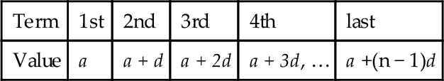
where:
n is the number of terms in the progression.
The sum Sn of all the terms is given by the average value of the terms times the number of terms; that is:
Sn=[(first+last)/2]×(numberofterms)=[(a+a+(n−1)d)/2]×n=(n/2)[2a+(n−1)d]
1.8.2 Geometric progressions
The relationship between consecutive numbers in a geometric progression is that they are connected by a common ratio. For the set of numbers 3, 6, 12, 24, 48, …, the series is obtained by multiplying the preceding number by 2. In general, when a is the first term and r is the common ratio, the geometric progression is of the form:
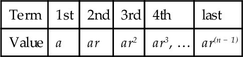
where:
n is the number of terms in the progression.
The sum Sn of all the terms may be found as follows:
Sn=a+ar+ar2+ar3+...+arn−1
Multiplying each term of equation (1) by r gives
rSn=ar+ar2+ar3+...+arn−1+arn
Subtracting equation (2) from (1) gives:
Sn(1−r)=a−arnSn=[a(1−r2)]/(1−r)
Alternatively, multiplying both numerator and denominator by −1 gives:
Sn=[a(rn−1)]/(r−1)
It is usual to use equation (3) when r<1 and (4) when r>1.
When −1>r>1,![]() each term of a geometric progression is smaller than the preceding term and the terms are said to converge. It is possible to find the sum of all the terms of a converging series. In this case, such a sum is called the sum to infinity. The term [a(1−rn)]/(1−r)
each term of a geometric progression is smaller than the preceding term and the terms are said to converge. It is possible to find the sum of all the terms of a converging series. In this case, such a sum is called the sum to infinity. The term [a(1−rn)]/(1−r)![]() can be rewritten as [a/(1−r)]−[arn/(1−r)].
can be rewritten as [a/(1−r)]−[arn/(1−r)].![]() Since r is less than 1, rn becomes smaller and smaller as n grows larger and larger. When n is very large, rn effectively becomes zero, and thus [arn/(1−r)].
Since r is less than 1, rn becomes smaller and smaller as n grows larger and larger. When n is very large, rn effectively becomes zero, and thus [arn/(1−r)].![]() becomes zero. It follows that the sum to infinity of a geometric progression is a/(1−r),
becomes zero. It follows that the sum to infinity of a geometric progression is a/(1−r),![]() which is valid when −1>r>1.
which is valid when −1>r>1.![]()
1.8.3 Harmonic progressions
The relationship between numbers in a harmonic progression is that the reciprocals of consecutive terms form an arithmetic progression. Thus for the arithmetic progression 1, 2, 3, 4, 5, …, the corresponding harmonic progression is 1, 1/2, 1/3, 1/4, 1/5, ….
1.9 Trigonometric formulae
1.9.1 Basic definitions
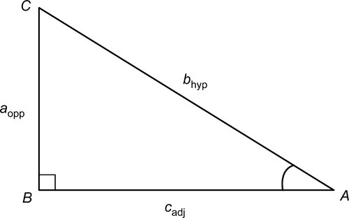
In the right-angled triangle shown below, a is the side opposite to angle A, b is the hypotenuse of the triangle and c is the side adjacent to angle A. By definition:
sinA=opp/hyp=a/bcosA=adj/hyp=c/btanA=opp/adj=a/ccosecA=hyp/opp=b/a=1/sinAsecA=hyp/adj=b/c=1/cosAcotA=adj/opp=c/a=1/tanA
1.9.2 Identities
sin2A+cos2A=11+tan2A=sec2A1+cot2A=cosec2Asin(−A)=−sinAcos(−A)=cosAtan(−A)=−tanA
1.9.3 Compound and double angle formulae
sin(A+B)=sinAcosB+cosAsinBsin(A−B)=sinAcosB−cosAsinBcos(A+B)=cosAcosB−sinAsinBcos(A−B)=cosAcosB+sinAsinBtan(A+B)=(tanA+tanB)/(1−tanAtanB)tan(A−B)=(tanA−tanB)/(1+tanAtanB)sin2A=2sinAcosAcos2A=cos2A−sin2A=2cos2A−1=1−2sin2Atan2A=(2tanA)/(1−tan2A)

1.9.4 ‘Product to sum’ formulae
sinAcosB=12[sin(A+B)+sin(A−B)]cosAsinB=12[sin(A+B)−sin(A−B)]cosAcosB=12[cos(A+B)+cos(A−B)]sinAsinB=12[cos(A+B)−cos(A−B)]
1.9.5 Triangle formulae

With reference to the above figure:
Sine rule:
a/sinA=b/sinB=c/sinC
![]()
Cosine rule:
a2=b2+c2−2bccosAb2=c2+a2−2cacosBc2=a2+b2−2abcosC
Area:
Area=12absinC=12bcsinA=12casinB
![]()
Also:
Area=√s(s−a)(s−a)(s−c)
![]()
where:
s is the semi-perimeter, that is, (a + b + c)/2.
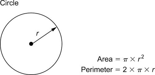
1.10 Circles: some definitions and properties
For a circle of diameter d and radius r:
The circumference is πd or 2πr
The area is πd2/4![]() or πr2.
or πr2.![]()
An arc of a circle is part of the circumference.
A tangent to a circle is a straight line which meets the circle at one point only. A radius drawn from the point where a tangent meets a circle is at right angles to the tangent.
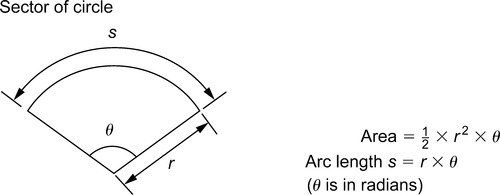
A sector of a circle is the area between an arc of the circle and two radii. The area of a sector is, 12r2θ,![]() where θ is the angle in radians between the radii.
where θ is the angle in radians between the radii.
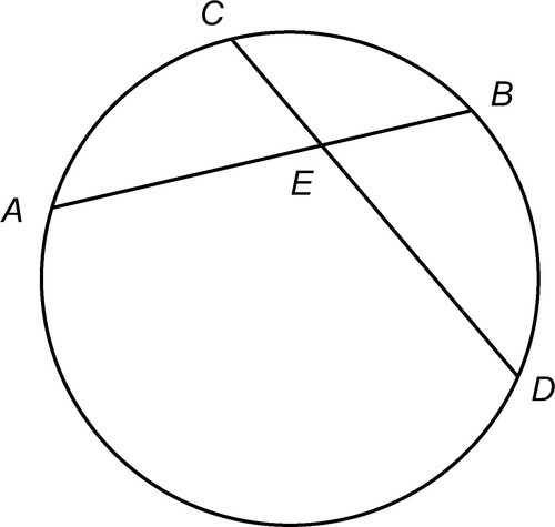
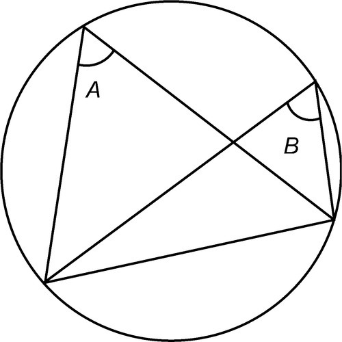
A chord is a straight line joining two points on the circumference of a circle. When two chords intersect, the product of the parts of one chord is equal to the products of the parts of the other chord. In the following figure, AE × BE = CE × ED.
A segment of a circle is the area bounded by a chord and an arc. Angles in the same segment of a circle are equal: in the following figure, angle A = angle B.
1.10.1 Circles: areas and circumferences
| Diameter | Area | Circumference |
| 1 | 0.7854 | 3.142 |
| 2 | 3.1416 | 6.283 |
| 3 | 7.0686 | 9.425 |
| 4 | 12.566 | 12.57 |
| 5 | 19.635 | 15.71 |
| 6 | 28.274 | 18.85 |
| 7 | 38.485 | 21.99 |
| 8 | 50.265 | 25.13 |
| 9 | 63.617 | 28.27 |
| 10 | 78.540 | 31.42 |
| 11 | 95.033 | 34.56 |
| 12 | 113.10 | 37.70 |
| 13 | 132.73 | 40.84 |
| 14 | 153.94 | 43.98 |
| 15 | 176.71 | 47.12 |
| 16 | 201.06 | 50.27 |
| 17 | 226.98 | 53.41 |
| 18 | 254.47 | 56.55 |
| 19 | 283.53 | 59.69 |
| 20 | 314.16 | 62.83 |
| 21 | 346.36 | 65.97 |
| 22 | 380.13 | 69.11 |
| 23 | 415.48 | 72.26 |
| 24 | 452.39 | 75.40 |
| 25 | 490.87 | 78.54 |
| 26 | 530.93 | 81.68 |
| 27 | 572.56 | 84.82 |
| 28 | 616.75 | 87.96 |
| 29 | 660.52 | 91.11 |
| 30 | 706.86 | 94.25 |
| 31 | 754.77 | 97.39 |
| 32 | 804.25 | 100.5 |
| 33 | 855.30 | 103.7 |
| 34 | 907.92 | 106.8 |
| 35 | 962.11 | 110.0 |
| 36 | 1017.9 | 113.1 |
| 37 | 1075.2 | 116.2 |
| 38 | 1134.1 | 119.4 |
| 39 | 1194.6 | 122.5 |
| 40 | 1256.6 | 125.7 |
| 41 | 1320.3 | 128.8 |
| 42 | 1385.4 | 131.9 |
| 43 | 1452.2 | 135.1 |
| 44 | 1520.5 | 138.2 |
| 45 | 1590.4 | 141.4 |
| 46 | 1661.9 | 144.5 |
| 47 | 1734.9 | 147.7 |
| 48 | 1809.6 | 150.8 |
| 49 | 1885.7 | 153.9 |
| 50 | 1963.5 | 157.1 |
| 51 | 2042.8 | 160.2 |
| 52 | 2123.7 | 163.4 |
| 53 | 2206.2 | 166.5 |
| 54 | 2290.2 | 169.6 |
| 55 | 2375.8 | 172.8 |
| 56 | 2463.0 | 175.9 |
| 57 | 2551.8 | 179.1 |
| 58 | 2642.1 | 182.2 |
| 59 | 2734.0 | 185.4 |
| 60 | 2827.4 | 188.4 |
| 61 | 2922.5 | 191.6 |
| 62 | 3019.1 | 194.8 |
| 63 | 3117.2 | 197.9 |
| 64 | 3217.0 | 201.1 |
| 65 | 3318.3 | 204.2 |
| 66 | 3421.2 | 207.3 |
| 67 | 3525.7 | 210.5 |
| 68 | 3631.7 | 213.6 |
| 69 | 3739.3 | 216.8 |
| 70 | 3848.5 | 219.9 |
| 71 | 3959.2 | 223.1 |
| 72 | 4071.5 | 226.2 |
| 73 | 4185.4 | 229.3 |
| 74 | 4300.8 | 232.5 |
| 75 | 4417.9 | 235.6 |
| 76 | 4536.5 | 238.8 |
| 77 | 4656.6 | 241.9 |
| 78 | 4778.4 | 245.0 |
| 79 | 4901.7 | 248.2 |
| 80 | 5026.5 | 251.3 |
| 81 | 5153.0 | 254.5 |
| 82 | 5381.0 | 257.6 |
| 83 | 5410.6 | 260.8 |
| 84 | 5541.8 | 263.9 |
| 85 | 5674.5 | 267.0 |
| 86 | 5808.8 | 270.2 |
| 87 | 5944.7 | 273.3 |
| 88 | 6082.1 | 276.5 |
| 89 | 6221.1 | 279.6 |
| 90 | 6361.7 | 282.7 |
| 91 | 6503.9 | 285.9 |
| 92 | 6647.6 | 289.0 |
| 93 | 6792.9 | 292.2 |
| 94 | 6939.8 | 295.3 |
| 95 | 7088.2 | 298.5 |
| 96 | 7238.2 | 301.6 |
| 97 | 7389.8 | 304.7 |
| 98 | 7543.0 | 307.9 |
| 99 | 7697.7 | 311.0 |
1.11 Quadratic equations
The solutions (roots) of a quadratic equation:
ax2+ bx + c= 0
![]()
are:
x=−b±√b2−4ac2a
![]()
1.12 Natural logarithms
The natural logarithm of a positive real number x is denoted by In x. It is defined to be a number such that:
elnx=x
![]()
where:
e = 2.1782 which is the base of natural logarithms.
Natural logarithms have the following properties:
In(xy)=Inx+InyIn(x/y)=Inx−InyInyx=xIny
1.13 Statistics: an introduction
1.13.1 Basic concepts
To understand the fairly advanced statistics underlying quality control, a certain basic level of statistics is assumed by most texts dealing with this subject. The brief introduction given below should help to lead readers into the various texts dealing with quality control.
The arithmetic mean, or mean, is the average value of a set of data. Its value can be found by adding together the values of the members of the set and then dividing by the number of members in the set. Mathematically:
X=(X1+X2+……+XN)/N
![]()
Thus the mean of the set of numbers 4, 6, 9, 3 and 8 is (4+6+9+3+8)/5=6.![]()
The median is either the middle value or the mean of the two middle values of a set of numbers arranged in order of magnitude. Thus the numbers 3, 4, 5, 6, 8, 9, 13 and 15 have a median value of (6+8)/2=7,![]() and the numbers 4, 5, 7, 9, 10, 11, 15, 17 and 19 have a median value of 10.
and the numbers 4, 5, 7, 9, 10, 11, 15, 17 and 19 have a median value of 10.
The mode is the value in a set of numbers which occurs most frequently. Thus the set 2, 3, 3, 4, 5, 6, 6, 6, 7, 8, 9 and 9 has a modal value of 6.
The range of a set of numbers is the difference between the largest value and the smallest value. Thus the range of the set of numbers 3, 2, 9, 7, 4, 1, 12, 3, 17 and 4 is 17 − 1 = 16.
The standard deviation, sometimes called the root mean square deviation, is defined by:
s=√[(X1−X)2+(X2−X)2+…+(XN−X)2]/N
![]()
Thus for the numbers 2, 5 and 11, the mean in (2 + 5 + 11)/3), that is 6. The standard deviation is:
s=√[(2−6)2+(5−6)2+(11−6)2]/3=√(16+1+25)/3=√14≈3.74
Usually s is used to denote the standard deviation of a population (the whole set of values) and σ is used to denote the standard deviation of a sample.
1.13.2 Probability
When an event can happen x ways out of a total of n possible and equally likely ways, the probability of the occurrence of the event is given by p=x/n.![]() The probability of an event occurring is therefore a number between 0 and 1. If q is the probability of an event not occurring it also follows that p+q=1.
The probability of an event occurring is therefore a number between 0 and 1. If q is the probability of an event not occurring it also follows that p+q=1.![]() Thus when a fair six-sided dice is thrown, the probability of getting a particular number, say a three, is 1/6, since there are six sides and the number three only appears on one of the six sides.
Thus when a fair six-sided dice is thrown, the probability of getting a particular number, say a three, is 1/6, since there are six sides and the number three only appears on one of the six sides.
1.13.3 Binomial distribution
The binomial distribution as applied to quality control may be stated as follows.
The probability of having 0, 1, 2, 3, …, n defective items in a sample of n items drawn at random from a large population, whose probability of a defective item is p and of a nondefective item is q, is given by the successive terms of the expansion of (q+p)n,![]() taking terms in succession from the right.
taking terms in succession from the right.
Thus if a sample of, say, four items is drawn at random from a machine producing an average of 5% defective items, the probability of having 0, 1, 2, 3 or 4 defective items in the sample can be determined as follows. By repeated multiplication:
(q+p)4=q4+4q3p+6q2p2+4qp3+p4
![]()
The values of q and p are q = 0.95 and p = 0.05. Thus:
(0.95+0.05)4=0.954+(4×0.953×0.05)+(6×0.952×0.052)+(4×0.95×0.053)+0.054=0.8145+0.1715+0.011354+…
![]()
This indicates that
(a) 81% of the samples taken are likely to have no defective items in them.
(b) 17% of the samples taken are likely to have one defective item.
(c) 1% of the samples taken are likely to have two defective items.
(d) There will hardly ever be three or four defective items in a sample.
As far as quality control is concerned, if by repeated sampling these percentages are roughly maintained, the inspector is satisfied that the machine is continuing to produce about 5% defective items. However, if the percentages alter then it is likely that the defect rate has also altered. Similarly, a customer receiving a large batch of items can, by random sampling, find the number of defective items in the samples and by using the binomial distribution can predict the probable number of defective items in the whole batch.
1.13.4 Poisson distribution
The calculations involved in a binomial distribution can be very long when the sample number n is larger than about six or seven, and an approximation to them can be obtained by using a Poisson distribution. A statement for this is:
When the chance of an event occurring at any instant is constant and the expectation np of the event occurring is λ, then the probabilities of the event occurring 0, 1, 2, 3, 4, … times are given by:
e−λ,λe−λ,λ2e−λ/2!,λ3e−λ/3!,λ4e−λ/4!,…
![]()
where:
e is the constant 2.71828 … and 2!=2 × 1, 3!=3 × 2 × 1, 4!=4 × 3 × 2 × 1, and so on (where 4! is read ‘four factorial').
Applying the Poisson distribution statement to the machine producing 5% defective items, used above to illustrate a use of the binomial distribution, gives:
expectation np 4 × 0.05 =0.2 probability of no defective items ise−λ=e−0.2=0.8187probability of one defective item isλe−λ=0.2e−0.2=0.1637probability of two defective items isλ2e−λ/2!=0.22e−0.2/2=0.0164
It can be seen that these probabilities of approximately 82%, 16% and 2% compare quite well with the results obtained previously.
1.13.5 Normal distribution
Data associated with measured quantities such as mass, length, time and temperature is called continuous, that is, the data can have any values between certain limits. Suppose that the lengths of items produced by a certain machine tool were plotted as a graph, as shown in the figure; then it is likely that the resulting shape would be mathematically definable. The shape is given by y=(1/σ)ez,![]() where z=(−X2/2σ2),
where z=(−X2/2σ2),![]() is the standard deviation of the data, and x is the frequency with which the data occurs. Such a curve is called a normal probability or a normal distribution curve.
is the standard deviation of the data, and x is the frequency with which the data occurs. Such a curve is called a normal probability or a normal distribution curve.
Important properties of this curve to quality control are:
(a) The area enclosed by the curve and vertical lines at ±1 standard deviation from the mean value is approximately 67% of the total area.

(b) The area enclosed by the curve and vertical lines at ±2 standard deviations from the mean value is approximately 95% of the total area.
(c) The area enclosed by the curve and vertical lines at ±3 standard deviations from the mean value is approximately 99.75% of the total area.
(d) The area enclosed by the curve is proportional to the frequency of the population.
To illustrate a use of these properties, consider a sample of 30 round items drawn at random from a batch of 1000 items produced by a machine. By measurement it is established that the mean diameter of the samples is 0.503 cm and that the standard deviation of the samples is 0.0005 cm. The normal distribution curve theory may be used to predict the reject rate if, say, only items having a diameter of 0.502-0.504 cm are acceptable. The range of items accepted is. Since the standard deviation is 0.0005 cm, this range corresponds to ±2 standard deviations. From (b) above, it follows that 95% of the items are acceptable, that is, that the sample is likely to have 28 to 29 acceptable items and the batch is likely to have 95% of 1000, that is, 950 acceptable items.
This example was selected to give exactly ±2 standard deviations. However, sets of tables are available of partial areas under the standard normal curve, which enable any standard deviation to be related to the area under the curve.
1.14 Differential calculus (Derivatives)
Ify=xnthendydx=nxn−1Ify=axnthendydx=anxn−1or

Iff(x)=axnthenf'(x)=anxn−1Ify=sinθthendydθ=cosθIfy=cosθthendydθ=−sinθIfy=tanθthendydθ=sec2θIfy=cotθthendydθ=cosec2θIfy=secθthendydθ=tanθsecθ=sinθcos2θIfy=cosecθthendydθ=−cotθcosecθ=−cosθsin2θIfy=sin−1xathendydx=1√a2−x2Ify=cos−1xathendydx=−1√a2−x2Ify=tan−1xathendydx=aa2+x2Ify=cot−1xathendydx=−aa2+x2Ify=sec−1xathendydx=ax√x2−a2Ify=cosec−1xathendydx=−ax√x2−a2Ify=exthendydx=exIfy=eaxthendydx=aeaxIfy=axthendydx=axlnaIfy=lnxthendydx=1x
Product rule
If y = uv where u and v are both functions of x, then dydx=udvdx+vdudx![]()
Quotient rule
If y=uv![]() where u and v are both functions of x, then dydx=vdudx−udvdxv2
where u and v are both functions of x, then dydx=vdudx−udvdxv2
Function of a function
If y is a function of x then dydx=dydu×dudx![]()
Successive differentiation
If y = f(x) then its first derivative is written dydx![]() or f″(x)
or f″(x)
If this expression is differentiated a second time then the second derivative is obtained and is written d2ydx2![]() or f״(x).
or f״(x).![]()
1.15 Integral calculus (Standard forms)
∫xndx=xn+1n+1+c(n≠−1)
![]()
Where
C = the constant of integration
∫axndx=axn−1n+1+c(n≠−1)∫cosθdθ=sinθ+c∫sinθdθ=−cosθ+c∫sec2θdθ=tanθ+c∫cosec2θdθ=−cotθ+c∫tanθsecθdθ=secθ+c∫cotθcosecθdθ=−cosecθ+c
∫dx√a2−x2=sin−1xa+c∫−dx√a2−x2=cos−1xa+c∫adxa2+x2=tan−1xa+c∫−adxa2+x2=cot−1xa+c∫adxx√x2−a2=sec−1xa+c∫−adxx√x2−a2=cosec−1xa+c∫exdx=ex+c∫eax=eaxa+c∫axdx=axIna+c∫dxx=lnx+c∫sinhxdx=coshx+c∫coshxdx=sinhx+c∫sech2dx=tanhx+c∫dx√a2+x2=sinh−1xa+corln[x+√x2+a2a]+c∫dx√x2−a2=cosh−1xa+corln[x+√x2−a2a]+c∫dxa2−x2=1atanhxa+cor12aIn(a+x)(a−x)+c

1.15.1 Integration by parts
∫udv=uv−∫vdu+c
![]()
1.15.2 Definite integrals
The foregoing integrals contain an arbitrary constant ‘c’ and are called indefinite integrals. Definite integrals are those to which limits are applied thus: [x]ba=(b)−(a),![]() therefore:
therefore:
y=3∫1x2dx=[x33+c]31=[333+c]−[133+c]=(9+c)−[13+c]=823

Note how the constant of integration (c) is eliminated in a definite integral.
1.16 Binomial theorem
(a+x)n=an+nan−1x+n(n−1)2!an−2x2+n(n−1)(n−2)3!an−3x3+…+xn
![]()
Where 3! is factorial 3 and equals 1 × 2 × 3.
1.17 Maclaurin’s theorem
f(x)=f(0)+xf′(0)+x22!f″(0)+……
![]()
1.18 Taylor’s theorem
f(x+h)=f(x)+hf′(x)+h22!f″(x)+……
![]()
For further information on Engineering Mathematics the reader is referred to the following Pocket Book: Newnes Engineering Mathematics Pocket Book, Third Edition, John Bird, 0750649925