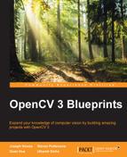
Given a dataset of face regions, we can use feature extraction to obtain the feature vector, which gives us the most important information from the expression. The following figure shows the process that we use in our implementation to extract features vectors:
The feature extraction process
In order to understand this chapter, you need to understand that the feature representation of the expression image is the distribution of image features over k clusters (k = 1000 in our implementation). We have implemented a few common types of features that are supported in OpenCV, such as SIFT, SURF, and some advanced features, such as DENSE-SIFT, KAZE, DAISY. Since these image features are computed at image key points such as corners, except for DENSE cases, the number of image features can vary between images. However, we want to have a fixed feature size for every image to perform classification, since we will apply machine learning classification techniques later. It is important that the feature size of the images is the same so that we can compare them to obtain the final result. Therefore, we apply a clustering technique (kmeans in our case) to separate the image feature space into a k cluster. The final feature representation for each image is the histogram of the image features over k bins. Moreover, in order to reduce the dimension of the final feature, we apply principle component analysis as a last step.
In the following sections, we will explain the process step by step. At the end of this section, we will show you how to use our implementation to obtain the final feature representation of the dataset.
At this point, we will assume that you have the face region for each image in the dataset. The next step is to extract the image features from these face regions. OpenCV provides good implementations of many well-known key point detection and feature description algorithms.
In this section, we will show you how to use some of these algorithms in our implementation.
We will use a function that takes current regions, a feature type, and returns a matrix with image features as rows:
Mat extractFeature(Mat face, string feature_name);
In this extractFeature function, we will extract image features from each Mat and return the descriptors. The implementation of extractFeature is simple, and shown here:
Mat extractFeature(Mat img, string feature_name){
    Mat descriptors;
    if(feature_name.compare("brisk") == 0){
        descriptors = extractBrisk(img);
    } else if(feature_name.compare("kaze") == 0){
        descriptors = extractKaze(img);
    } else if(feature_name.compare("sift") == 0){
        descriptors = extractSift(img);
    } else if(feature_name.compare("dense-sift") == 0){
        descriptors = extractDenseSift(img);
    } else if(feature_name.compare("daisy") == 0){
        descriptors = extractDaisy(img);
    }
    return descriptors;
}
In the above code, we call the corresponding function for each feature. For simplicity, we only use one feature each time. In this chapter, we will discuss two types of features:
- Contributed features: SIFT, DAISY, and DENSE SIFT. In OpenCV 3, the implementation of SIFT and SURF have been moved to the opencv_contrib module.
In this chapter, we will use SIFT features and the SIFT variant, DENSE SIFT.
- Advanced features: BRISK and KAZE. These features are a good alternative to SIFT and SURF in both performance and computation time. DAISY and KAZE are only available in OpenCV 3. DAISY is in opencv_contrib. KAZE is in the main OpenCV repository.
Let's take a look at SIFT features first.
In order to use SIFT features in OpenCV 3, you need to compile the opencv_contrib module with OpenCV.
The code to extract SIFT features is very simple:
Mat extractSift(Mat img){
    Mat descriptors;
    vector<KeyPoint> keypoints;

    Ptr<Feature2D> sift = xfeatures2d::SIFT::create();
    sift->detect(img, keypoints, Mat());
    sift->compute(img, keypoints, descriptors);

    return descriptors;
}
First, we create the Feature2D variable with xfeatures2d::SIFT::create() and use the detect function to obtain key points. The first parameter for the detection function is the image that we want to process. The second parameter is a vector to store detected key points. The third parameter is a mask specifying where to look for key points. We want to find key points in every position of the images so we just pass an empty Mat here.
Finally, we use the compute function to extract features descriptors at these key points. The computed descriptors are stored in the descriptors variable.
Next, let's take a look at the SURF features.
The code to obtain SURF features is more or less the same as that for SIFT features. We only change the namespace from SIFT to SURF:
Mat extractSurf(Mat img){
    Mat descriptors;
    vector<KeyPoint> keypoints;

    Ptr<Feature2D> surf = xfeatures2d::SURF::create();
    surf->detect(img, keypoints, Mat());
    surf->compute(img, keypoints, descriptors);

    return descriptors;
}
Let's now move on to DAISY.
DAISY is an improved version of the rotation-invariant BRISK descriptor and the LATCH binary descriptor that is comparable to the heavier and slower SURF. DAISY is only available in OpenCV 3 in the opencv_contrib module. The code to implement DAISY features is fairly similar to the Sift function. However, the DAISY class doesn't have a detect function so we will use SURF to detect key points and use DAISY to extract descriptors:
Mat extractDaisy(Mat img){
    Mat descriptors;
    vector<KeyPoint> keypoints;

    Ptr<FeatureDetector> surf = xfeatures2d::SURF::create();
    surf->detect(img, keypoints, Mat());
    Ptr<DescriptorExtractor> daisy = xfeatures2d::DAISY::create();
    daisy->compute(img, keypoints, descriptors);

    return descriptors;
}
It is now time to take a look at dense SIFT features.
Dense collects features at every location and scale in an image. There are plenty of applications where dense features are used. However, in OpenCV 3, the interface for extracting dense features has been removed. In this section, we show a simple approach to extracting dense features using the function in the OpenCV 2.4 source code to extract the vector of key points.
The function to extract dense Sift is similar to the Sift function:
Mat extractDenseSift(Mat img){
    Mat descriptors;
    vector<KeyPoint> keypoints;

    Ptr<Feature2D> sift = xfeatures2d::SIFT::create();
    createDenseKeyPoints(keypoints, img);
    sift->compute(img, keypoints, descriptors);

    return descriptors;
}
Instead of using the detect function, we can use the createDenseKeyPoints function to obtain key points. After that, we pass this dense key points vector to compute the function. The code for createDenseKeyPoints is obtained from the OpenCV 2.4 source code. You can find this code at modules/features2d/src/detectors.cpp in the OpenCV 2.4 repository:
void createDenseFeature(vector<KeyPoint> &keypoints, Mat image, float initFeatureScale=1.f, int featureScaleLevels=1,
                                    float featureScaleMul=0.1f,
                                    int initXyStep=6, int initImgBound=0,
                                    bool varyXyStepWithScale=true,
                                    bool varyImgBoundWithScale=false){
    float curScale = static_cast<float>(initFeatureScale);
    int curStep = initXyStep;
    int curBound = initImgBound;
    for( int curLevel = 0; curLevel < featureScaleLevels; curLevel++ )
    {
        for( int x = curBound; x < image.cols - curBound; x += curStep )
        {
            for( int y = curBound; y < image.rows - curBound; y += curStep )
            {
                keypoints.push_back( KeyPoint(static_cast<float>(x), static_cast<float>(y), curScale) );
            }
        }
        curScale = static_cast<float>(curScale * featureScaleMul);
        if( varyXyStepWithScale ) curStep = static_cast<int>( curStep * featureScaleMul + 0.5f );
        if( varyImgBoundWithScale ) curBound = static_cast<int>( curBound * featureScaleMul + 0.5f );
    }
}OpenCV 3 comes bundled with many new and advanced features. In our implementation, we will only use the BRISK and KAZE features. However, there are many other features in OpenCV.
Let us familiarize ourselves with the BRISK features.
BRISK is a new feature and a good alternative to SURF. It has been added to OpenCV since the 2.4.2 version. BRISK is under a BSD license so you don't have to worry about the patent problem, as with SIFT or SURF.
Mat extractBrisk(Mat img){
    Mat descriptors;
    vector<KeyPoint> keypoints;

    Ptr<DescriptorExtractor> brisk = BRISK::create();
    brisk->detect(img, keypoints, Mat());
    brisk->compute(img, keypoints, descriptors);

    return descriptors;
}
Note
There is an interesting article about all this, A battle of three descriptors: SURF, FREAK and BRISK, available at http://computer-vision-talks.com/articles/2012-08-18-a-battle-of-three-descriptors-surf-freak-and-brisk/.
Let's now move on and have a look at the KAZE features.
KAZE is a new feature in OpenCV 3. It produces the best results in many scenarios, especially with image matching problems, and it is comparable to SIFT. KAZE is in the OpenCV repository so you don't need opencv_contrib to use it. Apart from the high performance, one reason to use KAZE is that it is open source and you can use it freely in any commercial applications. The code to use this feature is very straightforward:
Mat extractKaze(Mat img){
    Mat descriptors;
    vector<KeyPoint> keypoints;

    Ptr<DescriptorExtractor> kaze = KAZE::create();
    kaze->detect(img, keypoints, Mat());
    kaze->compute(img, keypoints, descriptors);

    return descriptors;
}
Note
The image matching comparison between KAZE, SIFT, and SURF is available at the author repository: https://github.com/pablofdezalc/kaze
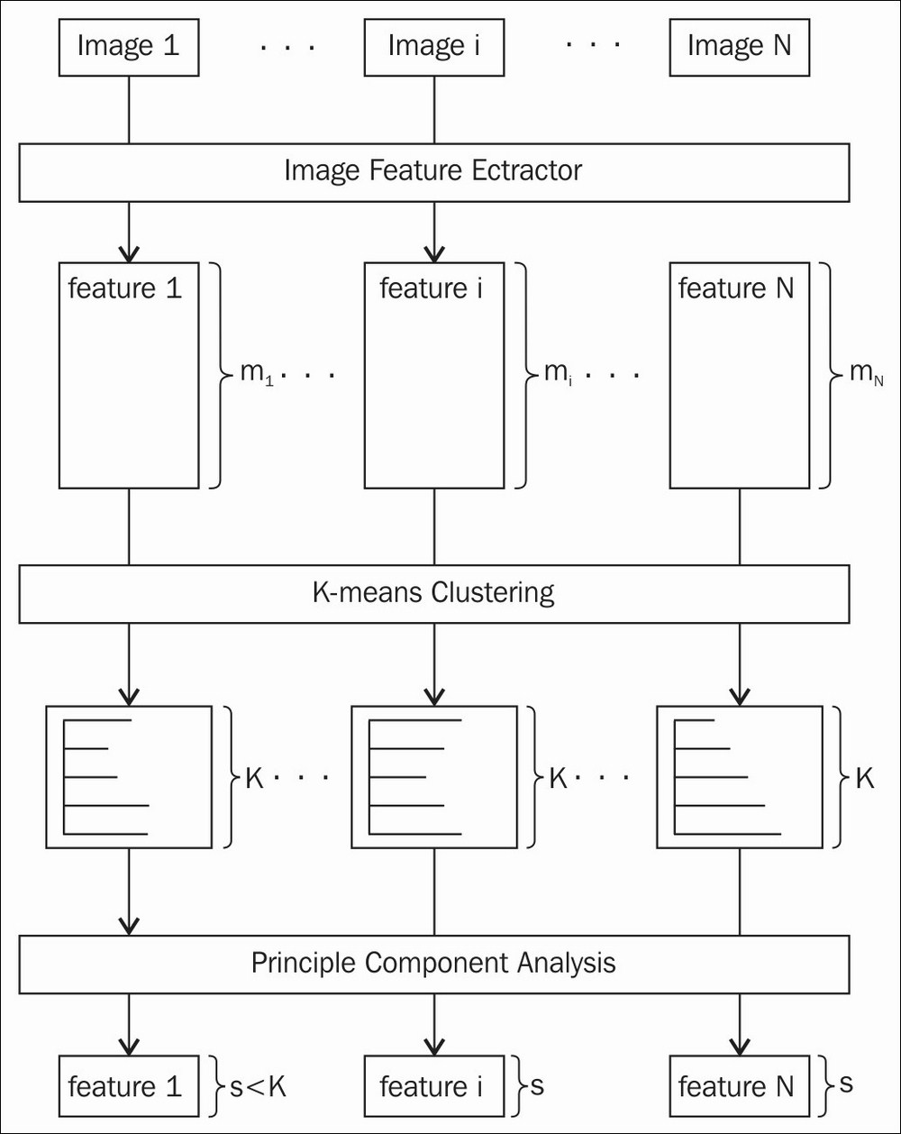
In the following figure, we visualize the position of key points for each feature type. We draw a circle at each key point; the radius of the circle specifies the scale of the image where the key point is extracted. You can see that the key points and the corresponding descriptors differ between these features. Therefore, the performance of the system will vary, based on the quality of the feature.
The feature extraction process
If you have followed the previous pseudo-code, you should now have a vector of descriptors. You can see that the size of descriptors varies between images. Since we want a fixed size of feature representation for each image, we will compute the distribution of feature representation over k clusters. In our implementation, we will use the kmeans clustering algorithm in the core module.
First, we assume that the descriptors of all the images are added to a vector, called features_vector. Then, we need to create a Mat rawFeatureData that will contain all of the image features as a row. In this case, num_of_feature is the total number of features in every image and image_feature_size is the size of each image feature. We choose the number of clusters based on experiment. We start with 100 and increase the number for a few iterations. It depends on the type of features and data, so you should try to change this variable to suit your situation. One downside of a large number of clusters is that the cost for computation with kmeans will be high. Moreover, if the number of clusters is too large, the feature vector will be too sparse and it may not be good for classification.
Mat rawFeatureData = Mat::zeros(num_of_feature, image_feature_size, CV_32FC1);
We need to copy the data from the vector of descriptors (features_vector in the code) to imageFeatureData:
int cur_idx = 0;
for(int i = 0 ; i < features_vector.size(); i++){
    features_vector[i].copyTo(rawFeatureData.rowRange(cur_idx, cur_idx + features_vector[i].rows));
    cur_idx += features_vector[i].rows;
}
Finally, we use the kmeans function to perform clustering on the data, as follows:
Mat labels, centers;
kmeans(rawFeatureData, k, labels, TermCriteria( TermCriteria::EPS+TermCriteria::COUNT, 100, 1.0), 3, KMEANS_PP_CENTERS, centers);
Let's discuss the parameters of the kmeans function:
double kmeans(InputArray data, int K, InputOutputArray bestLabels, TermCriteria criteria, int attempts, int flags, OutputArray centers=noArray())
- InputArray data: It contains all the samples as a row.
- int K: The number of clusters to split the samples ( k = 1000 in our implementation).
- InputOutputArray bestLabels: Integer array that contains the cluster indices for each sample.
- TermCriteria criteria: The algorithm termination criteria. This contains three parameters (
type,maxCount,epsilon). - Type: Type of termination criteria. There are three types:
- COUNT: Stop the algorithm after a number of iterations (
maxCount). - EPS: Stop the algorithm if the specified accuracy (epsilon) is reached.
- EPS+COUNT: Stop the algorithm if the COUNT and EPS conditions are fulfilled.
- COUNT: Stop the algorithm after a number of iterations (
- maxCount: It is the maximum number of iterations.
- epsilon: It is the required accuracy needed to stop the algorithm.
- int attemtps: It is the number of times the algorithm is executed with different initial centroids. The algorithm returns the labels that have the best compactness.
- int flags: This flag specifies how initial centroids are random. There are three types of flags. Normally,
KMEANS_RANDOM_CENTERSandKMEANS_PP_CENTERSare used. If you want to provide your own initial labels, you should useKMEANS_USE_INITIAL_LABELS. In this case, the algorithm will use your initial labels on the first attempt. For further attempts,KMEANS_*_CENTERSflags are applied. - OutputArray centers: It contains all cluster centroids, one row per each centroid.
- double compactness: It is the returned value of the function. This is the sum of the squared distance between each sample to the corresponding centroid.
We now have labels for every image feature in the dataset. The next step is to compute a fixed size feature for each image. With this in mind, we iterate through each image and create a feature vector of k elements, where k is the number of clusters.
Then, we iterate through the image features in the current image and increase the ith element of the feature vector where i is the label of the image features.
Imagine that we are trying to make a histogram representation of the features based on the k centroids. This method looks like a bag of words approach. For example, image X has 100 features and image Y has 10 features. We cannot compare them because they do not have the same size. However, if we make a histogram of 1,000 dimensions for each of them, they are then the same size and we can compare them easily.
In this section, we will use Principle Component Analysis (PCA) to reduce the dimension of the feature space. In the previous step, we have 1,000 dimensional feature vectors for each image. In our dataset, we only have 213 samples. Hence, the further classifiers tend to overfit the training data in high dimensional space. Therefore, we want to use PCA to obtain the most important dimension, which has the largest variance.
Next, we will show you how to use PCA in our system.
First, we assume that you can store all the features in a Mat named featureDataOverBins. The number of rows of this Mat should equal to the number of images in the dataset and the number of columns of this Mat should be 1,000. Each row in featureDataOverBins is a feature of an image.
Second, we create a PCA variable:
PCA pca(featureDataOverBins, cv::Mat(), CV_PCA_DATA_AS_ROW, 0.90);
The first parameter is the data that contains all the features. We don't have a pre-computed mean vector so the second parameter should be an empty Mat. The third parameter indicates that the feature vectors are stored as matrix rows. The final parameter specifies the percentage of variance that PCA should retain.
Finally, we need to project all the features from 1,000 dimensional feature spaces to a lower space. After the projection, we can save these features for further processes.
for(int i = 0 ; i < num_of_image; i++){
    Mat feature = pca.project(featureDataOverBins.row(i));
    // save the feature in FileStorage
}
The number of dimensions of the new features can be obtained by:
int feature_size = pca.eigenvectors.rows;
We have implemented the previous process to extract the fixed size feature for the dataset. Using the software is quite easy:
- Download the source code. Open the terminal and change directory to the source code folder.
- Build the software with
cmakeusing the following command:mkdir build && cd build && cmake .. && make - You can use the
feature_extractiontool as follows:./feature_extraction -feature <feature_name> -src <input_folder> -dest <output_folder>
The feature_extraction tool creates a YAML file in the output folder which contains the features and labels of every image in the dataset. The available parameters are:
feature_name: This can be sift, surf, opponent-sift, or opponent-surf. This is the name of the feature type which is used in the feature extraction process.input_folder: This has the absolute path to the location of facial components.output_folder: This has the absolute path to the folder where you want to keep the output file.
The structure of the output file is fairly simple.
We store the size of the feature, cluster centers, the number of images, the number of train and test images, the number of labels, and the corresponding label names. We also store PCA means, eigenvectors, and eigenvalues. The following figure shows a part of the YAML file:
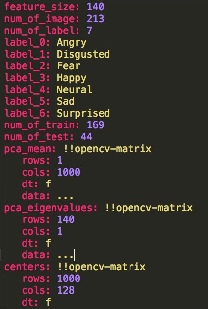
A part of the features.yml file
For each image, we store three variables, as follows:
image_feature_<idx>: It is a Mat that contains features of image idximage_label_<idx>: It is a label of the image idximage_is_train_<idx>: It is a Boolean specifying whether the image is used for training or not.