Once you have extracted the features for all the samples in the dataset, it is time to start the classification process. The target of this classification process is to learn how to make accurate predictions automatically based on the training examples. There are many approaches to this problem. In this section, we will talk about machine learning algorithms in OpenCV, including neural networks, support vector machines, and k-nearest neighbors.
Classification is considered supervised learning. In a classification problem, a correctly labelled training set is necessary. A model is produced during the training stage which makes predictions and is corrected when predictions are wrong. Then, the model is used for predicting in other applications. The model needs to be trained every time you have more training data. The following figure shows an overview of the classification process:
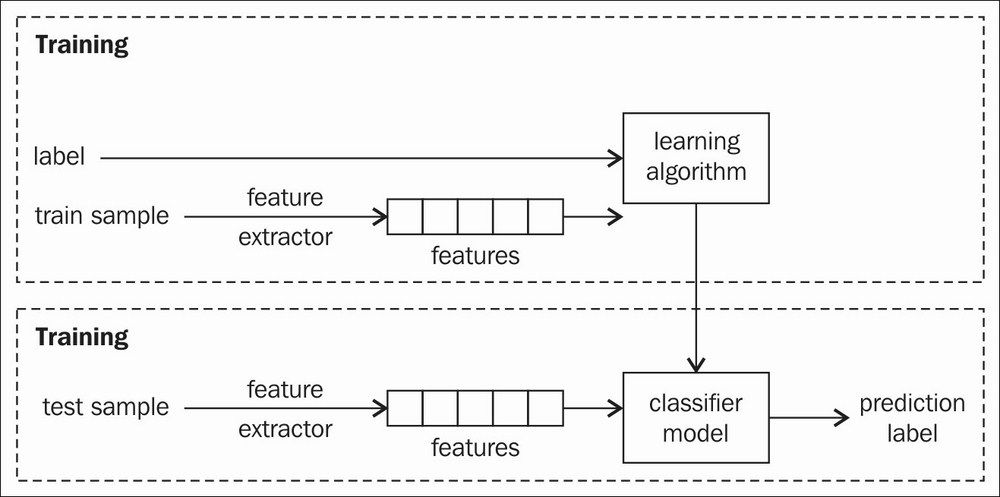
Overview of the classification process
The choice of learning algorithm to use is a critical step. There are a lot of solutions to the classification problem. In this section, we list some of the popular machine learning algorithms in OpenCV. The performance of each algorithm can vary between classification problems. You should make some evaluations and select the one that is the most appropriate for your problem to get the best results. It is essential as feature selection may affect the performance of the learning algorithm. Therefore, we also need to evaluate each learning algorithm with each different feature selection.
It is important that the dataset is separated into two parts, the training set and the testing set. We will use the training set for the learning stage and the testing set for the testing stage. In the testing stage, we want to test how the trained model predicts unseen samples. In other words, we want to test the generalization capability of the trained model. Therefore, it is important that the test samples are different from the trained samples. In our implementation, we will simply split the dataset into two parts. However, it is better if you use k-fold cross validation as mentioned in the Further reading section.
There is no accurate way to split the dataset into two parts. Common ratios are 80:20 and 70:30. Both the training set and the testing set should be selected randomly. If they have the same data, the evaluation is misleading. Basically, even if you achieve 99 percent accuracy on your testing set, the model can't work in the real world, where the data is different from the training data.
In our implementation of feature extraction, we have already randomly split the dataset and saved the selection in the YAML file.
A Support Vector Machine (SVM) is a supervised learning technique applicable to both classification and regression. Given labelled training data, the goal of SVM is to produce an optimal hyper plane which predicts the target value of a test sample with only test sample attributes. In other words, SVM generates a function to map between input and output based on labelled training data.
For example, let's assume that we want to find a line to separate two sets of 2D points. The following figure shows that there are several solutions to the problem:
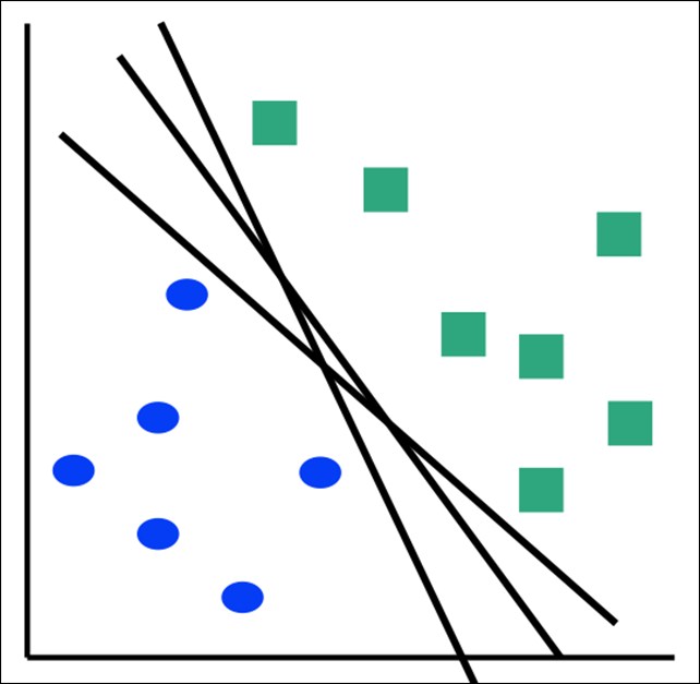
A lot of hyper planes can solve a problem
The goal of SVM is to find a hyper plane that maximizes the distances to the training samples. The distances are calculated to only support those vectors that are closest to the hyper plane. The following figure shows an optimal hyper plane to separate two sets of 2D points:
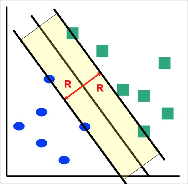
An optimal hyper plane that maximizes the distances to the training samples. R is the maximal margin
In the following sections, we will show you how to use SVM to train and test facial expression data.
One of the most difficult parts about training an SVM is parameters selection. It is not possible to explain everything without some deep understanding of how SVM works. Luckily, OpenCV implements a trainAuto method for automatic parameter estimation. If you have enough knowledge of SVM, you should try to use your own parameters. In this section, we will introduce the trainAuto method to give you an overview of SVM.
SVM is inherently a technique for building an optimal hyper plane in binary (2-class) classification. In our facial expression problem, we want to classify seven expressions. One-versus-all and one-versus-one are two common approaches that we can follow to use SVM in this problem. One-versus-all trains one SVM for each class. There are seven SVMs in our case. For class i, every sample with the label i is considered as positive and the rest of the samples are negative. This approach is prone to error when the dataset samples are imbalanced between classes. The one-versus-one approach trains an SVM for each different pairs of classes. The number of SVMs in total is N*(N-1)/2 SVMs. This means 21 SVMs in our case.
In OpenCV, you don't have to follow these approaches. OpenCV supports the training of one multiclass SVM. However, you should follow the above methods for better results. We will still use one multiclass SVM. The training and testing process will be simpler.
Next, we will demonstrate our implementation to solve the facial expression problem.
First, we create an instance of SVM:
Ptr<ml::SVM> svm = ml::SVM::create();
If you want to change parameters, you can call the set function in the svm variable, as shown:
svm->setType(SVM::C_SVC);
svm->setKernel(SVM::RBF);
- Type: It is the type of SVM formulation. There are five possible values:
C_SVC,NU_SVC,ONE_CLASS,EPS_SVR, andNU_SVR. However, in our multiclass classification, onlyC_SVCandNU_SVCare suitable. The difference between these two lies in the mathematical optimization problem. For now, we can just useC_SVC. - Kernel: It is the type of SVM kernel. There are four possible values:
LINEAR,POLY,RBF, andSIGMOID. The kernel is a function to map the training data to a higher dimensional space that makes data linearly separable. This is also known as Kernel Trick. Therefore, we can use SVM in non-linear cases with the support of the kernel. In our case, we choose the most commonly-used kernel, RBF. You can switch between these kernels and choose the best.
You can also set other parameters such as TermCriteria, Degree, Gamma. We are just using the default parameters.
Second, we create a variable of ml::TrainData to store all the training set data:
Ptr<ml::TrainData> trainData = ml::TrainData::create(train_features, ml::SampleTypes::ROW_SAMPLE, labels);
train_features: It is a Mat that contains each features vector as a row. The number of rows oftrain_featuresis the number of training samples, and the number of columns is the size of one features vector.SampleTypes::ROW_SAMPLE: It specifies that each features vector is in a row. If your features vectors are in columns, you should use COL_SAMPLE.train_labels: It is a Mat that contains labels for each training feature. In SVM,train_labelswill be a Nx1 matrix, N is the number of training samples. The value of each row is the truth label of the corresponding sample. At the time of writing, the type oftrain_labelsshould beCV_32S. Otherwise, you may encounter an error. The following code is what we use to create thetrain_labelsvariable:Mat train_labels = Mat::zeros( labels.rows, 1, CV_32S); for(int i = 0 ; i < labels.rows; i ++){ train_labels.at<unsigned int>(i, 0) = labels.at<int>(i, 0); }
Finally, we pass trainData to the trainAuto function so that OpenCV can select the best parameters automatically. The interface of the trainAuto function contains many other parameters. In order to keep things simple, we will use the default parameters:
svm->trainAuto(trainData);
After we've trained the SVM, we can pass a test sample to the predict function of the svm model and receive a label prediction, as follows:
float predict = svm->predict(sample);
In this case, the sample is a feature vector just like the feature vector in the training features. The response is the label of the sample.
OpenCV implements the most common type of artificial neural network, the multi-layer perceptron (MLP). A typical MLP consists of an input layer, an output layer, and one or more hidden layers. It is known as a supervised learning method because it needs a desired output to train. With enough data, MLP, given enough hidden layers, can approximate any function to any desired accuracy.
An MLP with a single hidden layer can be represented as it is in the following figure:
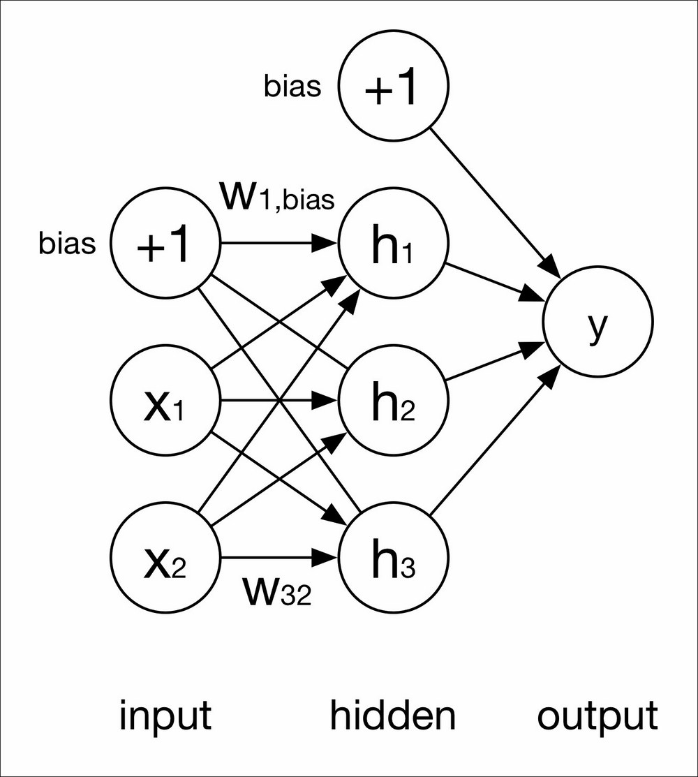
A single hidden layer perceptron
A detailed explanation and proof of how the MLP learns are out of the scope of this chapter. The idea is that the output of each neuron is a function of neurons from previous layers.
In the above single hidden layer MLP, we use the following notation:
Input layer: x1 x2
Hidden layer: h1 h2 h3
Output layer: y
Each connection between each neuron has a weight. The weight shown in the above figure is between neuron i (that is i = 3) in the current layer and neuron j (that is j = 2) in the previous layer is wij. Each neuron has a bias value 1 with a weight, wi,bias.
The output at neuron i is the result of an activation function f:
There are many types of activation functions. In OpenCV, there are three types of activation functions: Identity, Sigmoid, and Gaussian. However, the Gaussian function is not completely supported at the time of writing and the Identity function is not commonly used. We recommend that you use the default activation, Sigmoid.
In the following sections, we will show you how to train and test a multi-layer perceptron.
In the training stage, we first define the network and then train the network.
We will use a simple four layer neural network in our facial expression problem. The network has one input layer, two hidden layers, and one output layer.
First, we need to create a matrix to hold the layers definition. This matrix has four rows and one column:
Mat layers = Mat(3, 1, CV_32S);
Then, we assign the number of neurons for each layer, as follows:
layers.row(0) = Scalar(feature_size);
layers.row(1) = Scalar(20);
layers.row(2) = Scalar(num_of_labels);
In this network, the number of neurons for the input layer has to be equal to the number of elements of each feature vector, and number of neurons for the output layer is the number of facial expression labels (feature_size equals train_features.cols where train_features is the Mat that contains all features and num_of_labels equals 7 in our implementation).
The above parameters in our implementation are not optimal. You can try different values for different numbers of hidden layers and numbers of neurons. Remember that the number of hidden neurons should not be larger than the number of training samples. It is very difficult to choose the number of neurons in a hidden layer and the number of layers in your network. If you do some research, you can find several rules of thumb and diagnostic techniques. The best way to choose these parameters is experimentation. Basically, the more layers and hidden neurons there are, the more capacity you have in the network. However, more capacity may lead to overfitting. One of the most important rules is that the number of examples in the training set should be larger than the number of weights in the network. Based on our experience, you should start with one hidden layer with a small number of neurons and calculate the generalization error and training error. Then, you should modify the number of neurons and repeat the process.
However, in this case, we don't have much data. This makes the network hard to train. We may not add neurons and layers to improve the performance.
First, we create a network variable, ANN_MLP, and add the layers definition to the network:
Ptr<ml::ANN_MLP> mlp = ml::ANN_MLP::create();
mlp->setLayerSizes(layers);
Then, we need to prepare some parameters for training algorithms. There are two algorithms for training MLP: the back-propagation algorithm and the RPROP algorithm. RPROP is the default algorithm for training. There are many parameters for RPROP so we will use the back-propagation algorithm for simplicity.
Below is our code for setting parameters for the back-propagation algorithm:
mlp->setTrainMethod(ml::ANN_MLP::BACKPROP);
mlp->setActivationFunction(ml::ANN_MLP::SIGMOID_SYM, 0, 0);
mlp->setTermCriteria(TermCriteria(TermCriteria::EPS+TermCriteria::COUNT, 100000, 0.00001f));
We set the TrainMethod to BACKPROP to use the back-propagation algorithm. Select Sigmoid as the activation function There are three types of activation in OpenCV: IDENTITY, GAUSSIAN, and SIGMOID. You can go to the overview of this section for more details.
The final parameter is TermCriteria. This is the algorithm termination criteria. You can see an explanation of this parameter in the kmeans algorithm in the previous section.
Next, we create a TrainData variable to store all the training sets. The interface is the same as in the SVM section.
Ptr<ml::TrainData> trainData = ml::TrainData::create(train_features, ml::SampleTypes::ROW_SAMPLE, train_labels);
train_features is the Mat which stores all training samples as in the SVM section. However, train_labels is different:
train_features: This is a Mat that contains each features vector as a row as we did in the SVM. The number of rows oftrain_featuresis the number of training samples and the number of columns is the size of one features vector.train_labels: This is a Mat that contains labels for each training feature. Instead of the Nx1 matrix in SVM,train_labelsin MLP should be a NxM matrix, N is the number of training samples and M is the number of labels. If the feature at row i is classified as label j, the position (i, j) oftrain_labelswill be 1. Otherwise, the value will be zero. The code to create thetrain_labelsvariable is as follows:Mat train_labels = Mat::zeros( labels.rows, num_of_label, CV_32FC1); for(int i = 0 ; i < labels.rows; i ++){ int idx = labels.at<int>(i, 0); train_labels.at<float>(i, idx) = 1.0f; }
Finally, we train the network with the following code:
mlp->train(trainData);
The training process takes a few minutes to complete. If you have a lot of training data, it may take a few hours.
Once we have trained our MLP, the testing stage is very simple.
First, we create a Mat to store the response of the network. The response is an array, whose length is the number of labels.
Mat response(1, num_of_labels, CV_32FC1);
Then, we assume that we have a Mat, called sample, which contains a feature vector. In our facial expression case, its size should be 1x1000.
We can call the predict function of the mlp model to obtain the response, as follows:
mlp->predict(sample, response);
The predicted label of the input sample is the index of the maximum value in the response array. You can find the label by simply iterating through the array. The disadvantage of this type of response is that you have to apply a softmax function if you want a probability for each response. In other neural network frameworks, there is usually a softmax layer for this reason. However, the advantage of this type of response is that the magnitude of each response is retained.
K-Nearest Neighbors (KNN) is a very simple algorithm for machine learning but works very well in many practical problems. The idea of KNN is to classify an unknown example with the most common class among k-nearest known examples. KNN is also known as a non-parametric lazy learning algorithm. It means that KNN doesn't make any assumptions about the data distribution. The training process is very fast since it only caches all training examples. However, the testing process requires a lot of computation. The following figure demonstrates how KNN works in a 2D points case. The green dot is an unknown sample. KNN will find k-nearest known samples in space, (k = 5 in this example). There are three samples of red labels and two samples of blue labels. Therefore, the label for the prediction is red.
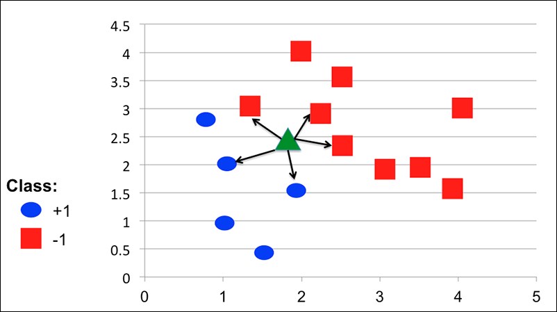
An explanation of how KNN predicts labels for unknown samples
The implementation of KNN algorithms is very simple. We only need three lines of code to train a KNN model:
Ptr<ml::KNearest> knn = ml::KNearest::create();
Ptr<ml::TrainData> trainData = ml::TrainData::create(train_features, ml::SampleTypes::ROW_SAMPLE, labels);
knn->train(trainData);
The preceding code is the same as with SVM:
train_features: This is a Mat that contains each features vector as a row. The number of rows intrain_featuresis the number of training samples and the number of columns is the size of one features vector.train_labels: This is a Mat that contains labels for each training feature. In KNN,train_labelsis a Nx1 matrix, N is the number of training samples. The value of each row is the truth label of the corresponding sample. The type of this Mat should beCV_32S.
The testing stage is very straightforward. We can just pass a feature vector to the findNearest method of the knn model and obtain the label:
Mat predictedLabels;
knn->findNearest(sample, K, predictedLabels);
The second parameter is the most important parameter. It is the number of maximum neighbors that may be used for classification. In theory, if there are an infinite number of samples available, a larger K always means a better classification. However, in our facial expression problem, we only have 213 samples in total and about 170 samples in the training set. Therefore, if we use a large K, KNN may end up looking for samples that are not neighbors. In our implementation, K equals 2.
The predicted labels are stored in the predictedLabels variable and can be obtained as follows:
float prediction = bestLabels.at<float>(0,0);
The Normal Bayes classifier is one of the simplest classifiers in OpenCV. The Normal Bayes classifier assumes that features vectors from each class are normally distributed, although not necessarily independently. This classifier is an effective classifier that can handle multiple classes. In the training step, the classifier estimates the mean and co-variance of the distribution for each class. In the testing step, the classifier computes the probability of the features to each class. In practice, we then test to see if the maximum probability is over a threshold. If it is, the label of the sample will be the class that has the maximum probability. Otherwise, we say that we can't recognize the sample.
OpenCV has already implemented this classifier in the ml module. In this section, we will show you the code to use the Normal Bayes classifier in our facial expression problem.
The code to implement the Normal Bayes classifier is the same as with SVM and KNN. We only need to call the create function to obtain the classifier and start the training process. All the other parameters are the same as with SVM and KNN.
Ptr<ml::NormalBayesClassifier> bayes = ml::NormalBayesClassifier::create();
Ptr<ml::TrainData> trainData = ml::TrainData::create(train_features, ml::SampleTypes::ROW_SAMPLE, labels);
bayes->train(trainData);
The code to test a sample with the Normal Bayes classifier is a little different from previous methods:
- First, we need to create two Mats to store the output class and probability:
Mat output, outputProb;
- Then, we call the
predictProbfunction of the model:bayes->predictProb(sample, output, outputProb);
- The computed probability is stored in
outputProband the corresponding label can be retrieved as:unsigned int label = output.at<unsigned int>(0, 0);
We have implemented the above process to perform classification with a training set. Using the software is quite easy:
- Download the source code. Open the terminal and change directory to the source code folder.
- Build the software with
cmakeusing the follow command:mkdir build && cd build && cmake .. && make - You can use the
traintool as follows:./train -algo <algorithm_name> -src <input_features> -dest <output_folder>
The train tool performs the training process and outputs the accuracy on the console. The learned model will be saved to the output folder for further use as model.yml. Furthermore, kmeans centers and pca information from features extraction are also saved in features_extraction.yml. The available parameters are:
algorithm_name: This can bemlp,svm,knn,bayes. This is the name of the learning algorithm.input_features: This is the absolute path to the location of the YAML features file from theprepare_datasettool.output_folder: This is the absolute path to the folder where you want to keep the output model.