In the section that discusses the mathematical basis, we found several unknown camera parameters. These parameters need to be figured out so we can process each image and stabilize it. As with any calibration process, we need to use a predefined scene. Using this scene and a relative handshake, we will try to estimate the unknown parameters.
- Focal length of the lens
- Delay between gyroscope and frame timestamps
- Bias in the gyroscope
- Duration of the rolling shutter
It is often possible to detect the focal length of a phone camera (in terms of millimeters) using the platform API (getFocalLength() for Android). However, we're interested in the camera space focal length. This number is a product of the physical focal length and a conversion ratio that depends on the image resolution and the physical size of the camera sensor, which might differ across cameras. It is also possible to find the conversion ratio by trigonometry if the field of view (getVerticalViewAngle() and getHorizontalViewAngle() for Android) is known for a sensor and lens setup. However, we'll just leave it as an unknown and let the calibration find it for us.
Note
If you're interested in more information on this, refer to Chapter 5, Combining Image Tracking with 3D Rendering, of PacktPub's Android Application Programming with OpenCV.
We need to estimate the delay between gyro and frame timestamps to improve the quality of the output on sharp turns. This also offsets any lag introduced by the phone when recording the video.
Rolling shutter effects are visible at high speed and the estimated parameter tries to correct these.
It is possible to calculate these parameters with a short clip that's shaky. We use a feature detector from OpenCV to do this.
Note
During this phase, we'll be using Python. The SciPy library provides us with mathematical functions that we can use out of the box. It is possible to implement these on your own, but that would require a more in-depth explanation of how mathematical optimization works. Along with this, we'll use Matplotlib to generate graphs.
We'll set up three key data structures: first, the unknown parameters, second, something to read the gyro data file generated by the Android app, and third, a representation of the video being processed.
The first structure is to store the estimates from the calibration. It contains four values:
- An estimate of the focal length of the camera (in camera units, not physical units)
- The delay between the gyroscope timestamps and the frame timestamps
- The gyroscope bias
- The rolling shutter estimated
Let's start by creating a new file called calibration.py.
import sys, numpy

class CalibrationParameters(object):
    def __init__(self):
        self.f = 0.0
        self.td = 0.0
        self.gb = (0.0, 0.0, 0.0)
self.ts = 0.0Next, we'll define a class to read in the .csv file generated by the Android app.
class GyroscopeDataFile(object):
    def __init__(self, filepath):
        self.filepath = filepath
        self.omega = {}

    def getfile_object(self):
        return open(self.filepath)
We initialize the class with two main variables: the file path to read, and a dictionary of angular velocities. This dictionary will store mappings between the timestamp and the angular velocity at that instant. We'll eventually need to calculate actual angles from the angular velocity, but that will happen outside this class.
Now we add the parse method. This method will actually read the file and populate the Omega dictionary.
    def parse(self):
        with self._get_file_object() as fp:
            firstline = fp.readline().strip()
            if not firstline == 'utk':
                raise Exception("The first line isn't valid")
We validate that the first line of the csv file matches our expectation. If not, the csv file was probably not compatible and will error out over the next few lines.
            for line in fp.readlines():
                line = line.strip()
                parts = line.split(",")
Here, we initiate a loop over the entire file. The strip function removed any additional whitespace (tabs, spaces, newline characters, among others) that might be stored in the file.
After removing the whitespace, we split the string with commas (this is a comma-separated file!).
                timestamp = int(parts[3])
                ox = float(parts[0])
                oy = float(parts[1])
                oz = float(parts[2])
                print("%s: %s, %s, %s" % (timestamp,
                                          ox,
                                          oy,
                                          oz))
                self.omega[timestamp] = (ox, oy, oz)
    return
Information read from the file is plain strings so we convert that into the appropriate numeric type and store it in self.omega. We're now ready to parse the csv files and get started with numeric calculations.
Before we do that, we'll define a few more useful functions.
    def get_timestamps(self):
        return sorted(self.omega.keys())

    def get_signal(self, index):
        return [self.omega[k][index] for k in self.get_timestamps()]
The get_timestamps method on this class will return a sorted list of timestamps. Building on this, we also define a function called get_signal. The angular velocity is composed of three signals. These signals are packed together in self.omega. The get_signal function lets us extract a specific component of the signal.
For example, get_signal(0) returns the X component of angular velocity.
    def get_signal_x(self):
        return self.get_signal(0)

    def get_signal_y(self):
        return self.get_signal(1)

    def get_signal_z(self):
        return self.get_signal(2)
These utility functions return only the specific signal we're looking at. We'll be using these signals to smooth out individual signals, calculate the angle, and so on.
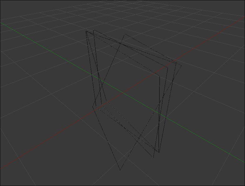
Another issue we need to address is that the timestamps are discrete. For example, we might have angular velocities at timestamp N and the next reading might exist at N+500000 (remember, the timestamps are in nanoseconds). However, the video file might have a frame at N+250000. We need a way to interpolate between two angular velocity readings.
We'll use simple linear interpolation to estimate the angular velocity at any given moment.
    def fetch_approximate_omega(self, timestamp):
        if timestamp in self.omega:
            return self.omega[timestamp]
This method takes in a timestamp and returns the estimated angular velocity. If the exact timestamp already exists, there is no estimation to do.
        i = 0
        sorted_timestamps = self.get_timestamps()
        for ts in sorted_timestamps:
            if  ts > timestamp:
                break
            i += 1
Here we're walking over the timestamps and finding the timestamp that is closest to the one requested.
        t_previous = sorted_timestamps[i]
        t_current = sorted_timestamps[i+1]
        dt = float(t_current – t_previous)
        slope = (timestamp – t_previous) / dt

        est_x = self.omega[t_previous][0]*(1-slope) + self.omega[t_current][0]*slope
        est_y = self.omega[t_previous][1]*(1-slope) + self.omega[t_current][1]*slope
        est_z = self.omega[t_previous][2]*(1-slope) + self.omega[t_current][2]*slope
        return (est_x, est_y, est_z)
Once we have the two closest timestamps (i and i+1 in the list sorted_timestamps), we're ready to start linear interpolation. We calculate the estimated X, Y, and Z angular velocities and return these values.
This finishes our work on reading the gyroscope file!
We'll also create a new class that lets us treat the entire video sequence as a single entity. We'll extract useful information from the video in a single pass and store it for future reference, making our code both faster and more memory efficient.
class GyroVideo(object):def__init__(self, mp4):
        self.mp4 = mp4
        self.frameInfo = []
        self.numFrames = 0
        self.duration = 0
        self.frameWidth = 0
        self.frameHeight = 0
We initialize the class with some variables we'll be using throughout. Most of the variables are self-explanatory. frameInfo stores details about every frame—like the timestamp of a given frame and keypoints (useful for calibration).
    def read_video(self, skip_keypoints=False):
        vidcap = cv2.VideoCapture(self.mp4)
        success, frame = vidcap.read()
        prev_frame = None
        previous_timestamp = 0
        frameCount = 0
We define a new method that will do all the heavy lifting for us. We start by creating the OpenCV video reading object (VideoCapture) and try to read a single frame.
        while success:
            current_timestamp = vidcap.get(0) * 1000 * 1000
            print "Processing frame#%d (%f ns)" % (frameCount, current_timestamp)
The get method on a VideoCapture object returns information about the video sequence. Zero (0) happens to be the constant for fetching the timestamp in milliseconds. We convert this into nanoseconds and print out a helpful message!
            if not prev_frame:
                self.frameInfo.append({'keypoints': None,
                                       'timestamp': current_timestamp})
                prev_frame = frame
                previous_timestamp = current_timestamp
                continue
If this is the first frame being read, we won't have a previous frame. We're also not interested in storing keypoints for the first frame. So we just move on to the next frame.
            if skip_keypoints:
                self.frameInfo.append({'keypoints': None,
                                       'timestamp': current_timestamp})
                continue
If you set the skip_keypoints parameter to true, it'll just store the timestamps of each frame. You might then use this parameter to read a video after you've already calibrated your device and already have the values of the various unknowns.
            old_gray = cv2.cvtColor(prev_frame, cv2.COLOR_BGR2GRAY)
            new_gray = cv2.cvtColor(frame, cv2.COLOR_BGR2GRAY)

            old_corners = cv2.goodFeaturesToTrack(old_gray, 1000, 0.3, 30)
We convert the previous and the current frame into grayscale and extract some good features to track. We'll use these features and track them in the new frame. This gives us a visual estimate of how the orientation of the camera changed. We already have the gyroscope data for this; we just need to calibrate some unknowns. We achieve this by using the visual estimate.
            if old_corners == None:
                self.frameInfo.append({'keypoints': None,
                                       'timestamp': current_timestamp})
                frameCount += 1
                previous_timestamp = current_timestamp
                prev_frame = frame
                success, frame = vidcap.read()
                continue
If no corners were found in the old frame, that's not a good sign. Was it a very blurry frame? Were there no good features to track? So we simply skip processing it.
If we did find keypoints to track, we use optical flow to identify where they are in the new frame:
            new_corners, status, err = cv2.calcOpticalFlowPyrLK(old_gray,
                                           new_gray,
                                           old_corners,
                                           None,
                                           winSize=(15,15)
                                           maxLevel=2,
                                           criteria=(cv2.TERM_CRITERIA_EPS
                                                     | cv2.TERM_CRITERIA_COUNT,
                                                     10, 0.03))
This gives us the position of the corners in the new frame. We can then estimate the motion that happened between the previous frame and the current, and correlate it with the gyroscope data.
A common issue with goodFeaturesToTrack is that the features aren't robust. They often move around, losing the position they were tracking. To get around this, we add another test just to ensure such random outliers don't make it to the calibration phase. This is done with the help of RANSAC.
Note
RANSAC stands for Random Sample Consensus. The key idea of RANSAC is that the given dataset contains a set of inliers that fit perfectly to a given model. It gives you the set of points that most closely satisfy a given constraint. In our case, these inliers would account for the points moving from one set of positions to another. It does not matter how numerous the outliers of the data set are.
OpenCV comes with a utility function to calculate the perspective transform between two frames. While the transform is being estimated, the function also tries to figure out which points are outliers. We'll hook into this functionality for our purposes too!
            if len(old_corners) > 4:
                homography, mask = cv2.findHomography(old_corners, new_corners,
                                                      cv2.RANSAC, 5.0)
                mask = mask.ravel()
                new_corners_homography = [new_corners[i] for i in xrange(len(mask)) if mask[i] == 1])
                old_corners_homography = [old_corners[i] for i in xrange(len(mask)) if mask[i] == 1])
                new_corners_homography = numpy.asarray(new_corners_homography)
                old_corners_homography = numpy.asarray(old_corners_homography)
            else:
                new_corners_homography = new_corners
                old_corners_homography = old_corners
We need at least four keypoints to calculate the perspective transform between two frames. If there aren't enough points, we just store whatever we have. We get a better result if there are more points and some are eliminated.
            self.frameInfo.append({'keypoints': (old_corners_homography,
                                                 new_corners_homography),
                                   'timestamp': current_timestamp})
            frameCount += 1
            previous_timestamp = current_timestamp
            prev_frame = frame
            success, frame = vidcap.read()
        self.numFrames = frameCount
        self.duration = current_timstamp
        return
Once we have everything figured out, we just store it in the frame information list. And this marks the end of our method!
Let's take a look at how we rotate frames to stabilize them.
Before we get into how images can be rotated for our project, let's look at rotating images in general. The goal is to produce images like the one below:
Rotating an image in 2D is simple, there's only one axis. A 2D rotation can be achieved by using an affine transform.
In our project, we need to rotate images around all three axes. An affine transform is not sufficient to produce these, so we need to go towards a perspective transform. Also, rotations are linear transformations; this means we can split an arbitrary rotation into its component X, Y, and Z rotations and use that to compose the rotation.
To achieve this, we'll use the OpenCV Rodrigues function call to generate these transformation matrices. Let's start by writing a function that arbitrarily rotates an image.
def rotateImage(src, rx, ry, rz, f, dx=0, dy=0, dz=0, convertToRadians=False):
    if convertToRadians:
        rx = (rx) * math.pi / 180
        ry = (ry) * math.pi / 180
        rz = (rz) * math.pi / 180

    rx = float(rx)
    ry = float(ry)
    rz = float(rz)
This method accepts a source image that needs to be rotated, the three rotation angles, an optional translation, the focal length in pixels, and whether the angles are in radians or not. If the angles are in degrees, we need to convert them to radians. We also force convert these into float.
Next, we'll calculate the width and the height of the source image. These, along with the focal length, are used to transform the rotation matrix (which is in real world space) into image space.
    w = src.shape[1]
    h = src.shape[0]
Now, we use the Rodrigues function to generate the rotation matrix:
    smallR = cv2.Rodrigues(np.array([rx, ry, rz]))[0]
    R = numpy.array([ [smallR[0][0], smallR[0][1], smallR[0][2], 0],
                      [smallR[1][0], smallR[1][1], smallR[1][2], 0],
                      [smallR[2][0], smallR[2][1], smallR[2][2], 0],
                      [0,            0,            0,            1]])
The Rodrigues function takes a vector (a list) that contains the three rotation angles and returns the rotation matrix. The matrix returned is a 3x3 matrix. We'll convert that into a 4x4 homogeneous matrix so that we can apply transformations to it.
We now apply a simple translation to the matrix. The translation matrix is easily evaluated as follows:
    x = numpy.array([[1.0, 0,   0,   dx],
                     [0,   1.0, 0,   dy],
                     [0,   0,   1.0, dz],
                     [0,   0,   0,   1]])
    T = numpy.asmatrix(x)
Until now, all transformations have happened in world space. We need to change these into image space. This is accomplished by the simple pinhole model of a camera.
    c = numpy.array([[f, 0, w/2, 0],
                     [0, f, h/2, 0],
                     [0, 0, 1,   0]])
    cameraMatrix = numpy.asmatrix(c)
Combining these transforms is straightforward:
transform = cameraMatrix * (T*R)
This matrix can now be used in OpenCV's warpPerspective method to rotate the source image.
    output = cv2.warpPerspective(src, transform, (w, h))
    return output
The output of this isn't exactly what you want though, the images are rotated about (0, 0) in the image. We need to rotate the image about the center. To achieve this, we need to insert an additional translation matrix right before the rotations happen.
    w = src.shape[1]
    h = src.shape[0]

    # New code:
    x = numpy.array([ [1, 0, -w/2],
                      [0, 1, -h/2],
                      [0, 0, 0],
                      [0, 0, 1]]
    A1 = numpy.asmatrix(x)
    ...
Now, we insert the matrix A1 at the very beginning:
transform = cameraMatrix * (T*(R*A1))
Now images should rotate around the center; this is exactly what we want and is a self-contained method that we can use to rotate images arbitrarily in 3D space using OpenCV.
Rotating an image with a single rotation vector is quite straightforward. In this section, we'll extend that method so it is better suited for our project.
We have two data sources active when recording a video: the image capture and the gyroscope trace. These are captured at different rates—images every few milliseconds and gyroscope signals every few microseconds. To calculate the exact rotation required to stabilize an image, we need to accumulate the rotation of dozens of gyroscope signals. This means that the rotation matrix needs to have information on several different gyroscope data samples.
Also, the gyroscope and image sensors are not in sync; we will need to use linear interpolation on the gyroscope signals to bring them in sync.
Let's write a function that returns the transformation matrix.
def getAccumulatedRotation(w, h,
                           theta_x, theta_y, theta_z, timestamps,
                           prev, current,
                           f,
                           gyro_delay=None, gyro_drift=None, shutter_duration=None):
    if not gyro_delay:
        gyro_delay = 0

    if not gyro_drift:
        gyro_drift = (0, 0, 0)

    if not shutter_duration:
        shutter_duration = 0
This function takes a lot of parameters. Let's go over each of them:
w,h: We need to know the size of the image to convert it from world space to image space.- theta_*: Currently, we have access to angular velocity. From there, we can evaluate actual angles and that is what this function accepts as parameters.
- Timestamps: The time each sample was taken.
prev,current: Accumulate rotations between these timestamps. This will usually provide the timestamp of the previous frame and the current frame.f,gyro_delay,gyro_drift, andshutter_durationare used to improve the estimate of the rotation matrix. The last three of these are optional (and they get set to zero if you don't pass them).
From the previous section, we know that we need to start by translating (or we'll get rotations about (0, 0)).
    x = numpy.array([[1, 0, -w/2],
                  [0, 1, -h/2],
                  [0, 0, 0],
                  [0, 0, 1]])
    A1 = numpy.asmatrix(x)
    transform = A1.copy()
We'll use the "transform" matrix to accumulate rotations across multiple gyroscope samples.
Next, we offset the timestamps by using gyro_delay. This is just adding (or subtracting, based on the sign of its value) to the timestamp.
    prev = prev + gyro_delay
    current = current + gyro_delay
    if prev in timestamps and current in timestamps:
        start_timestamp = prev
        end_timestamp = current
    else:
        (rot, start_timestamp, t_next) = fetch_closest_trio(theta_x,
                                                            theta_y,
                                                            theta_z,
                                                            timestamps,
                                                            prev)
        (rot, end_timestamp, t_next) = fetch_closest_trio(theta_x,
                                                          theta_y,
                                                          theta_z,
                                                          timestamps,
                                                          current)
If the updated prev and current values exist in the timestamps (meaning we have values captured from the sensor at that time instant) – great! No need to interpolate. Otherwise, we use the function fetch_closest_trio to interpolate the signals to the given timestamp.
This helper function returns three things:
- The interpolated rotation for the requested timestamp
- The closest timestamp in the sensor data
- The timestamp right after it
We use start_timestamp and end_timestamp for iterating now.
    for time in xrange(timestamps.index(start_timestamp), timestamps.index(end_timestamp)):
        time_shifted = timestamps[time] + gyro_delay
        trio, t_previous, t_current = fetch_closest_trio(theta_x, theta_y, theta_z, timestamps, time_shifted)
        gyro_drifted = (float(trio[0] + gyro_drift[0]),
                        float(trio[1] + gyro_drift[1]),
                        float(trio[2] + gyro_drift[2]))
We iterate over each timestamp in the physical data. We add the gyroscope delay and use that to fetch the closest (interpolated) signals. Once that's done, we add the gyroscope drift per component. This is just a constant that should be added to compensate for errors in the gyroscope.
Using these rotation angles, we now calculate the rotation matrix, as in the previous section.
        smallR = cv2.Rodrigues(numpy.array([-float(gyro_drifted[1]),
                                            -float(gyro_drifted[0]),
                                            -float(gyro_drifted[2])]))[0]
        R = numpy.array([[smallR[0][0], smallR[0][1], smallR[0][2], 0],
                         [smallR[1][0], smallR[1][1], smallR[1][2], 0],
                         [smallR[2][0], smallR[2][1], smallR[2][2], 0],
                         [0,            0,            0,            1]])
        transform = R * transform
This piece of code is almost the same as that in the previous section. There are a few key differences though. Firstly, we're providing negative values to Rodrigues. This is to negate the effect of motion. Secondly, the X and Y values are swapped. (gyro_drifted[1] comes first, followed by gyro_drifted[0]). This is required because the axes of the gyroscope and the ones used by these matrices are different.
This completes the iteration over the gyroscope samples between the specified timestamps. To complete this, we need to translate in the Z direction just like in the previous section. Since this can be hardcoded, let's do that:
    x = numpy.array([[1, 0, 0, 0],
                     [0, 1, 0, 0],
                     [0, 0, 1, f],
                     [0, 0, 0, 1]])
    T = numpy.asmatrix(x)
We also need to use the camera matrix to convert from world space to image space.
    x = numpy.array([[f, 0, w/2, 0],
                     [0, f, h/2, 0],
                     [0, 0, 1,   0]])
    A2 = numpy.asmatrix(x)
    transform = A2 * (T*transform)
    return transform
We first translate in the Z direction and then convert to image space. This section essentially lets you rotate frames of your video with the gyroscope parameters.
With our data structures ready, we're in a good place to start the key piece of this project. The calibration builds on all the previously mentioned classes.
As always, we'll create a new class which encapsulates all the calibration-related tasks.
class CalibrateGyroStabilize(object):
    def __init__(self, mp4, csv):
        self.mp4 = mp4
        self.csv = csv
The object requires two things: the video file and the gyroscope data file. These get stored in the object.
Before jumping directly into the calibration method, let's create some utility functions that will be helpful when calibrating.
    def get_gaussian_kernel(sigma2, v1, v2, normalize=True):
        gauss = [math.exp(-(float(x*x) / sigma2)) for x in range(v1, v2+1)]

        if normalize:
            total = sum(guass)
            gauss = [x/total for x in gauss]

        return gauss
This method generates a Gaussian kernel of a given size. We'll use this to smooth out the angular velocity signals in a bit.
    def gaussian_filter(input_array):
        sigma = 10000
        r = 256
        kernel = get_gaussian_kernel(sigma, -r, r)
        return numpy.convolve(input_array, kernel, 'same')
This function does the actual smoothing of a signal. Given an input signal, it generates the Gaussian kernel and convolves it with the input signal.
Note
Convolutions are a mathematical tool to produce new functions. You can think of the gyroscope signal as a function; you give it a timestamp and it returns a value. To smooth it out, we need to combine it with another function. This function, called the Gaussian function, is a smooth bell curve. Both these functions have different time ranges on which they operate (the gyroscope function might return values between a time of 0 seconds and 50 seconds while the Gaussian function might just work for a time of 0 seconds to 5 seconds). Convolving these two functions produces a third function that behaves a bit like both, thereby effectively smoothing out the minor variations in the gyroscope signal.
Next, we write a function that calculates an error score giving two sets of points. This will be a building block in estimating how good the calibration has been.
    def calcErrorScore(set1, set2):
        if len(set1) != len(set2):
            raise Exception("The given sets need to have the exact same length")

        score = 0
        for first, second in zip(set1.tolist(), set2.tolist()):
            diff_x = math.pow(first[0][0] – second[0][0], 2)
            diff_y = math.pow(first[0][1] – second[0][1], 2)
            score += math.sqrt(diff_x + diff_y)

        return score
This error score is straightforward: you have two lists of points and you calculate the distance between the corresponding points on the two lists and sum it up. A higher error score means the points on the two lists don't correspond perfectly.
This method, however, only gives us the error on a single frame. We're concerned about errors across the whole video. We therefore write another method.
    def calcErrorAcrossVideo(videoObj, theta, timestamp, focal_length, gyro_delay=None, gyro_drift=None, rolling_shutter=None):
        total_error = 0
        for frameCount in xrange(videoObj.numFrames):
            frameInfo = videoObj.frameInfo[frameCount]
            current_timestamp = frameInfo['timestamp']

            if frameCount == 0:
                previous_timestamp = current_timestamp
                continue
            keypoints = frameInfo['keypoints']

            if not keypoints:
                continue
We pass in the video object and all the details we have estimated (the theta, timestamps, focal length, gyroscope delay, and so on). With these details, we try to do the video stabilization and see what differences exists between the visually tracked keypoints and the gyroscope-based transformations.
Since we're calculating the error across the whole video, we need to iterate over each frame. If the frame's information does not have any keypoints in it, we simply ignore the frame. If the frame does have keypoints, here's what we do:
            old_corners = frameInfo['keypoints'][0]
            new_corners = frameInfo['keypoints'][1]
            transform = getAccumulatedRotation(videoObj.frameWidth,
                                               videoObj.frameHeight,
                                               theta[0], theta[1], theta[2],
                                               timestamps,
                                               int(previous_timestamp),
                                               int(current_timestamp),
                                               focal_length,
                                               gyro_delay,
                                               gyro_drift,
                                               rolling_shutter)
The getAccumulatedRotation function is something we'll write soon. The key idea of the function is to return a transformation matrix for the given theta (the angles we need to rotate to stabilize the video). We can apply this transform to old_corners and compare it to new_corners.
Since new_corners was obtained visually, it is the ground truth. We want getAccumulatedRotation to return a transformation that matches the visual ground truth perfectly. This means the error between new_corners and the transformed old_corners should be minimal. This is where calcErrorScore helps us:
            transformed_corners = cv2.perspectiveTransform(old_corners, transform)
            error = calcErrorScore(new_corners, transformed_corners)
            total_error += error
            previous_timestamp = current_timestamp
        return total_error
We're ready to calculate the error across the whole video! Now let's move to the calibration function:
    def calibrate(self):
        gdf = GyroscopeDataFile(csv)
        gdf.parse()

        signal_x = gdf.get_signal_x()
        signal_y = gdf.get_signal_y()
        signal_z = gdf.get_signal_z()
        timestamps = gdf.get_timestamps()
The first step is to smooth out the noise in the angular velocity signals. This is the desired signal with smooth motion.
        smooth_signal_x = self.gaussian_filter(signal_x)
        smooth_signal_y = self.gaussian_filter(signal_y)
        smooth_signal_z = self.gaussian_filter(signal_z)
We'll be writing the gaussian_filter method soon; for now, let's just keep in mind that it returns a smoothed out signal.
Next, we calculate the difference between the physical signal and the desired signal. We need to do this separately for each component.
        g = [ [], [] [] ]
        g[0] = numpy.subtract(signal_x, smooth_signal_x).tolist()
        g[1] = numpy.subtract(signal_y, smooth_signal_y).tolist()
        g[2] = numpy.subtract(signal_z, smooth_signal_z).tolist()
We also need to calculate the delta between the timestamps. We'll be using this for integration.
dgt = self.diff(timestamps)
Next, we integrate the angular velocities to get actual angles. Integration introduces errors into our equations but that's okay. It is good enough for our purposes.
        theta = [ [], [], [] ]
        for component in [0, 1, 2]:
            sum_of_consecutives = numpy.add( g[component][:-1], g[component][1:])
            dx_0 = numpy.divide(sum_of_consecutives, 2 * 1000000000)
            num_0 = numpy.multipy(dx_0, dgt)
            theta[component] = [0]
            theta[component].extend(numpy.cumsum(num_0))
And that's it. We have calculated the amount of theta that will stabilize the image! However, this is purely from the gyroscope's view. We still need to calculate the unknowns so that we can use these thetas to stabilize the image.
To do this, we initialize some of the unknowns as variables with an arbitrary initial value (0 in most cases). Also, we load the video and process the keypoint information.
        focal_length = 1080.0
        gyro_delay = 0
        gyro_drift = (0, 0, 0)
        shutter_duration = 0

        videoObj = GyroVideo(mp4)
        videoObj.read_video()
Now, we use SciPy's optimize method to minimize the error. To do this, we must first convert these unknowns into a Numpy array.
        parameters = numpy.asarray([focal_length,
                                    gyro_delay,
                                    gyro_drift[0], gyro_drift[1], gyro_drift[2]])
Since we've not yet incorporated fixing the rolling shutter, we ignore that in the parameters list. Next, we call the actual optimization function:
        result = scipy.optimize.minimize(self.calcErrorAcrossVideoObjective,
                                         parameters,
                                         (videoObj, theta, timestamps),
                                         'Nelder-Mead')
Executing this function takes a few seconds, but it produces the values of the unknowns for us. We can then extract these from the result as follows:
        focal_length = result['x'][0]
        gyro_delay = result['x'][1]
        gyro_drift = ( result['x'][2], result['x'][3], result['x'][4] )
        print "Focal length = %f" % focal_length
        print "Gyro delay   = %f" % gyro_delay
        print "Gyro drift   = (%f, %f, %f)" % gyro_drift
With this, we're done with calibration! All we need to do is return all the relevant calculations we've done just now.
return (delta_theta, timestamps, focal_length, gyro_delay, gyro_drift, shutter_duration)
And that's a wrap!
In the previous section, we calculated all the unknowns in our equations. Now, we can go ahead with fixing the shaky video.
We'll start off by creating a new method called stabilize_video. This method will take a video file and a corresponding csv file.
def stabilize_video(mp4, csv):
    calib_obj = CalibrateGyroStabilize(mp4, csv)
We create an object of the calibration class we just defined and pass it the required information. Now, we just need to call the calibrate function.
delta_theta, timestamps, focal_length, gyro_delay, gyro_drift, shutter_duration = calib_obj.calibrate()
This method call may take a while to execute, but we need to run this only once for every device. Once calculated, we can store these values in a text file and read them from there.
Once we have estimated all the unknowns, we start by reading the video file for each frame.
vidcap = cv2.VideoCapture(mp4)
Now we start iterating over each frame and correcting the rotations.
    frameCount = 0
    success, frame = vidcap.read()
    previous_timestamp = 0
    while success:
        print "Processing frame %d" % frameCount
Next, we fetch the timestamp from the video stream and use that to fetch the closest rotation sample.
current_timestamp = vidcap.get(cv2.CAP_PROP_POS_MSEC) * 1000 * 1000
The VideoCapture class returns timestamps in milliseconds. We convert that into nanoseconds to keep consistent units.
rot, prev, current = fetch_closest_trio(delta_theta[0],delta_theta[1],delta_theta[2],timestamps,current_timestamps)
With these pieces, we now fetch the accumulated rotation.
rot = accumulateRotation(frame, delta_theta[0],delta_theta[1],delta_theta[2],timestamps, previous_timestamp,prev,focal_length,gyro_delay,gyro_drift,shutter_duration)
Next, we write the transformed frame into a file and move on to the next frame:
        cv2.imwrite("/tmp/rotated%04d.png" % frameCount, rot)
        frameCount += 1
        previous_timestamp = prev
        success, frame = vidcap.read()
    return
And this finishes our simple function to negate the shakiness of the device. Once we have all the images, we can combine them into a single video with ffmpeg.
ffmpeg -f image2 -i image%04d.jpg output.mp4
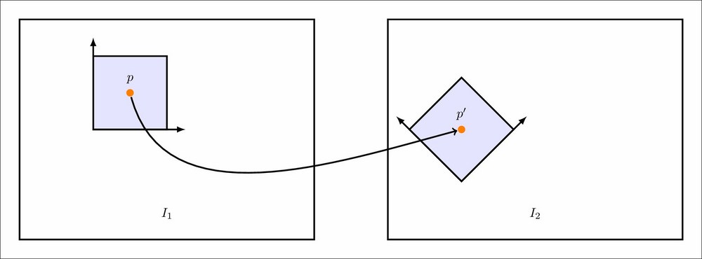
The effectiveness of the calibration depends on how accurately it can replicate motion on the video. For any frame, we have matching keypoints in the previous and current frames. This gives a sense of the general motion of the scene.
Using the estimated parameters, if we are able to use previous frames' keypoints to generate the current frames' keypoints, we can assume the calibration has been successful.