
Chapter 17. Cars and Hovercraft
What cars and hovercraft have in common is that they operate in an essentially 2D manner. Unless they have jumped a ramp, both vehicles remain on the ground or water plane. In this chapter we’ll discuss the forces behind each vehicle’s method of travel and discuss how to accurately model them in your simulations.
Cars
In the following sections we want to discuss certain aspects of the physics behind automobile motion. Like the previous four chapters, the purpose of this chapter is to explain, by example, certain physical phenomena. We also want to give you a basic understanding of the mechanics involved in automobile motion in case you want to simulate one in your games. In keeping with the theme of this book, we’ll be talking about mechanics in the sense of rigid-body motion, and not in the sense of how an internal combustion engine works, or how power is transferred through the transmission system to the wheels, etc. Those are all internal to the car as a rigid body, and we’ll focus on the external forces. We will, however, discuss how the torque applied to the drive wheel is translated to a force that pushes the car along.
Resistance
Before we talk about why cars move forward, let’s talk about what slows them down. When a car drives down a road, it experiences two main components of resistance that try to slow it down. The first component is aerodynamic drag, and the second is called rolling resistance. The total resistance felt by the car is the sum of these two components:
| Rtotal = Rair + Rrolling |
The aerodynamic drag is primarily skin friction and pressure drag similar to that experienced by the projectiles discussed in Chapter 6, and the planes and boats discussed in earlier chapters. Here again, you can use the familiar drag formula:
| Rair = (1/2) ρ V2 Sp Cd |
Here ρ (rho) is the mass density of air, V is the speed of the car, Sp is the projected frontal area of the car normal to the direction of V, and Cd is the drag coefficient. Typical ranges of drag coefficients for different types of vehicles are 0.29 to 0.4 for sports cars, 0.43 to 0.5 for pickup trucks, 0.6 to 0.9 for tractor-trailers, and 0.4 to 0.5 for the average economy car. Drag coefficient is a function of the shape of the vehicle—that is, the degree of boxiness or streamline. Streamlined body styles have lower drag coefficients; for example, the Chevy Corvette has a low drag coefficient of 0.29, while the typical tractor-trailer without fairings has a high drag coefficient of up to 0.9. You can use these coefficients in your simulations to tune the behavior of different types and shapes of vehicles.
When a tire rolls on a road, it experiences rolling resistance, which tends to retard its motion. Rolling resistance is not frictional resistance, but instead has to do with the deformation of the tire while rolling. It’s a difficult quantity to calculate theoretically since it’s a function of a number of complicated factors—such as tire and road deformation, the pressure over the contact area of the tire, the elastic properties of the tire and road materials, the roughness of the tire and road surfaces, and tire pressure, to name a few—so instead you’ll have to rely on an empirical formula. The formula to use is as follows:
| Rrolling = Cr w |
This gives you the rolling resistance per tire, where w is the weight supported by the tire, and Cr is the coefficient of rolling resistance. Cr is simply the ratio of the rolling resistance force to the weight supported by the tire. Luckily for you, tire manufacturers generally provide the coefficient of rolling resistance for their tires under design conditions. Typical car tires have a Cr of about 0.015, while truck tires fall within the range of 0.006 to 0.01. If you assume that a car has four identical tires, then you can estimate the total rolling resistance for the car by substituting the total car weight for w in the preceding equation.
Power
Now that you know how to calculate the total resistance on your car, you can easily calculate the power required to overcome the resistance at a given speed. Power is a measure of the amount of work done by a force, or torque, over time. Mechanical work done by a force is equal to the force times the distance an object moves under the action of that force. It’s expressed in units such as foot-pounds. Since power is a measure of work done over time, its units are, for example, foot-pounds per second. Usually power in the context of car engine output is expressed in units of horsepower, where 1 horsepower equals 550 ft-lbs/s.
To calculate the horsepower required to overcome total resistance at a given speed, you simply use this formula:
| P = (Rtotal V) / 550 |
Here P is power in units of horsepower, and Rtotal is the total resistance corresponding to the car’s speed, V. Note, in this equation Rtotal must be in pound units and V must be in units of feet per second.
Now this is not the engine output power required to reach the speed V for your car; rather, it is the required power delivered by the drive wheel to reach the speed V. The installed engine power will be higher for several reasons. First, there will be mechanical losses associated with delivering the power from the engine through the transmission and drive train to the tire. The power will actually reach the tire in the form of torque, which given the radius of the tire will create a force Fw that will overcome the total resistance. This force is calculated as follows:
| Fw = Tw/r |
Here Fw is the force delivered by the tire to the road to push the car along, Tw is the torque on the tire, and r is the radius of the tire. The second reason the installed engine power will be greater is because some engine power will be transferred to other systems in the car. For example, power is required to charge the battery and to run the air conditioner.
Stopping Distance
Under normal conditions, stopping distance is a function of the braking system and how hard the driver applies the brakes: the harder the brakes are applied, the shorter the stopping distance. That’s not the case when the tires start to skid. Under skidding conditions, stopping distance is a function of the frictional force that develops between the tires and the road, in addition to the inclination of the roadway. If the car is traveling uphill, the skidding distance will be shorter because gravity helps slow the car, while it will tend to accelerate the car and increase the skidding distance when the car is traveling downhill.
There’s a simple formula that considers these factors that you can use to calculate skidding distance:
| ds = V2 / [2g ( µ cos φ + sin φ)] |
Here ds is the skidding distance, g the acceleration due to gravity, µ the coefficient of friction between the tires and road, V the initial speed of the car, and φ the inclination of the roadway (where a positive angle means uphill and a negative angle means downhill). Note that this equation does not take into account any aerodynamic drag that will help slow the car down.
The coefficient of friction will vary depending on the condition of the tires and surface of the road, but for rubber on pavement the dynamic friction coefficient is typically around 0.4, while the static coefficient is around 0.55.
When calculating the actual frictional force between the tire and road, say in a real-time simulation, you’ll use the same formula that we showed you in Chapter 3:
| Ff = µ W |
Here Ff is the friction force applied to each tire, assuming it’s not rolling, and W is the weight supported by each tire. If you assume that all tires are identical, then you can use the total weight of the car in the preceding formula to determine the total friction force applied to all tires.
Steering
When you turn the steering wheel of a car, the front wheels exert a side force such that the car starts to turn. In terms of Euler angles, this would be yaw, although Euler angles aren’t usually used in discussions about turning cars. Even if the car’s speed is constant, it experiences acceleration due to the fact that its velocity vector has changed direction. Remember, acceleration is the time rate of change in velocity, which has both magnitude and direction.
For a car to maintain its curved path, there must be a centripetal force (“center seeking” in Greek) that acts on the car. When riding in a turning car, you feel an apparent centrifugal acceleration, or force directed away from the center of the turn. This acceleration is really a result of inertia, the tendency of your body and the car to continue on their original path, and is not a real force acting on the car or your body. The real force is the centripetal force, and without it your car would continue on its straight path and not along the curve.
One of the most important aspects of racing is taking turns as fast as possible but without losing control. The longer you can wait to decelerate for the turn, and the sooner you can start accelerating again, the higher your average speed will be. It is interesting to note that when people ride in racecars, what really surprises them isn’t the acceleration but the massive decelerations they can create through braking forces. A Formula One car regularly experiences decelerations of 4g, with 5–6g being the extreme value for certain race courses. Most road-legal sports cars can achieve about 1g of braking force. This allows the racecars to maintain speed until just entering the corner.
When you turn the steering wheel in a car, the tires produce a centripetal force toward the center of the curve via friction with the surface of the road. It follows that the maximum static frictional force between the tires and the road must exceed the required centripetal force. Mathematically, this takes on the following inequality:
| µ sN > mv2/r |
Centripetal acceleration is the square of the tangential velocity, v, divided by the radius of the turn, r. This multiplied by mass of the vehicle, m, gives the force required to make a turn. The available force is the static coefficient of friction times the normal force, N. Rewriting this formula, we can develop a simplified maximum cornering speed as follows:
| vlimit < |
If this speed is exceeded, the cornering force will exceed the static coefficient of friction and the tires will begin to slide. It may be tempting to replace the normal force, N, with the weight of the vehicle (mass times gravity) and cancel out the mass of the car, but the normal force may not always be simplified as such, as we’ll discuss in a moment. Also, in real life, the weight of a vehicle is rarely evenly distributed among all four tires and is definitely not when the car is acceleration or decelerating. In general, acceleration causes a weight shift to the aft tires, and deceleration causes weight to shift to the forward tires. This is important because, depending on where the weight is, the front or back tires will tend to have less available friction. If one or the other sets of tires begins to slide, the car will either understeer or oversteer (see Figure 17-1).
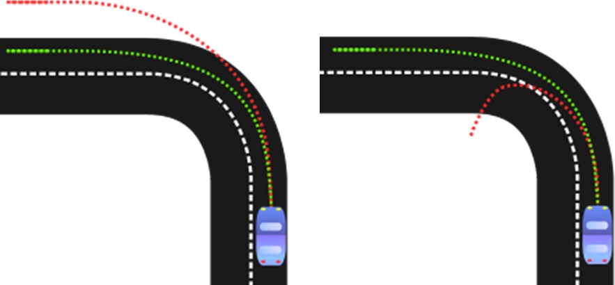
If the front wheels slide, the car understeers and the arc is larger than the driver intended. This is commonly caused by traveling too fast through a corner and trying to take the corner too tightly. However, if the driver breaks hard or even just lets off the gas, there will be a weight shift forward. This will keep the forward wheels from slipping but if too aggressive will cause the rear wheels to slip as weight is transferred away from them. This causes the car to turn more than the driver intended, and can even result in a spin. These two conditions limit the speed at which a car can complete a turn and also the amount of deceleration the car can handle once the turn is initiated.
To increase the limit speed, vlimit, we must increase the normal force. We could do so by increasing the car’s mass, but this would have negative effects on the car’s ability to accelerate or decelerate. A better solution is the use of aerodynamic features to create what is called downforce. You may have seen racecars or even street cars with large wing-like features called spoilers on their trunks. Formula 1 cars also have wing-like appendages on the front of the car. These are like the wings of an airplane but inverted so that instead of pulling the vehicle up, they actually push the vehicle down. These wings, therefore, increase the normal force, and their effects are proportional to speed so that more downforce is available at higher speeds...just when you need it. In fact, some very fast cars create so much downforce that if the road were inverted, the car would remain glued to the pavement and be able to drive upside-down.
The trade-off for this increased cornering limit speed is increased drag caused by the airfoils. This limits the top speed of the vehicle in areas of road that have no corners. It is good practice to allow users to select an angle of attack for their vehicle’s airfoils. This forces them to choose between the option of higher top speed with slower cornering or faster cornering with lower top speed.
You may notice that on some raceways, the corners are not flat. This is called roadway bank or superelevation. In a corner where the car would normally skid, the superelevation helps keep the car in the turn because as the car is inclined, a force component develops that acts toward the center of curvature of the turn (see Figure 17-2).
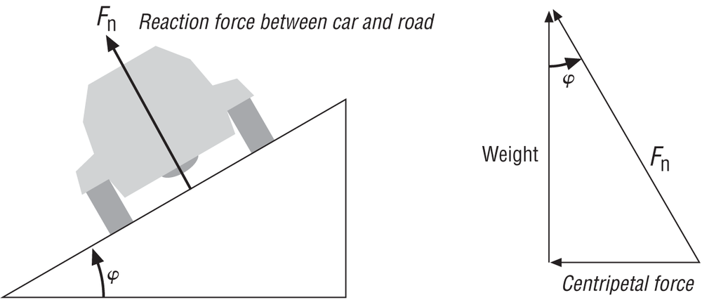
The following simple formula relates the superelevation angle of a roadway to the speed of the car and the coefficient of friction between the tires and road:
| tan φ = Vt2/(g r) – µs |
Here, φ is the superelevation angle (as shown in Figure 17-2), Vt is the tangential component of velocity of the car going around the turn, g is the acceleration due to gravity, r is the radius of the curve, and µs is the static coefficient of friction between the tires and the road. If you know φ, r, and µ, then you can calculate the speed at which the car will begin to slip out of the turn and off the road.
Vehicle dynamics is a complex field, and if you are interested in a highly realistic driving simulation game, we recommend reading up on the subject. A good starting place is Fundamentals of Vehicle Dynamics by Thomas Gillespie (Society of Automobile Engineers).
Hovercraft
Hovercraft, or air cushion vehicles (ACVs), have made their way into a video game or two recently. Their appeal seems to stem from their futuristic aura, high speed, and levitating ability, which lets them go anywhere. In real life, hovercraft have been around since the 1950s and have been used in combat, search and rescue, cargo transport, ferrying, and recreational roles. They come in all shapes and sizes, but they all pretty much work the same, with the basic idea of getting the craft off the land or water to reduce its drag. In Chapter 9, we touched on what forces you have to model when considering hovercraft, and now we’ll talk about them in more detail.
How Hovercraft Work
The first hovercraft designs pumped air through an annular nozzle around the periphery of the craft (see Figure 17-3). Large fans are used to feed the air through the nozzle under the craft. This jet of air creates a region of relatively high pressure over the area underneath the craft, which results in a net lifting force. The lifting force must equal the weight of the craft if it is to attain hovering flight. This sort of lifting is known as aerostatic lift. The hover height is limited by the amount of power available and the lifting fan’s ability to pump enough air through the nozzle: the higher the hover height, the greater the power demand.
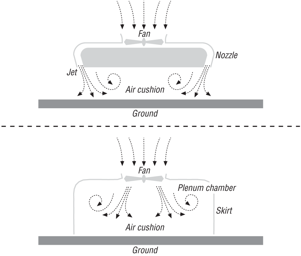
This approach proved impractical because hover heights were very limited and made the clearance between the hard structure of the craft and the ground (or water) too small to overcome all but the smallest obstacles. The solution to this problem was to fit a flexible skirt around the craft to contain the air cushion in what’s called the plenum chamber (see Figure 17-3). This approach extended the clearance between the ground and the hard structure of the craft significantly even though the gap between the bottom of the skirt and the ground was very small. This is the basic configuration of most hovercraft in operation today, although there are all sorts of skirt designs. Some of these skirts are simple curtains, while others are sophisticated pressurized bag and finger arrangements. The end result is that hovercraft fitted with skirts can clear relatively large obstacles without damage to their hard structure, and the skirt simply distorts and conforms to the terrain over which the craft operates.
The actual calculation of the aerostatic lift force is fairly complicated because the pressure distribution within the air cushion is nonuniform and because you must also take into account the performance of the lift fan system. There are theories available to treat both the annular jet and plenum chamber configurations, but they are beyond the scope of this book. Besides, for a game simulation, what’s important is that you realize that the lift force must equal the weight of the craft in order for it to maintain equilibrium in hovering flight.
Ideally, the ability of a hovercraft to eliminate contact with the ground (or water) over which it operates means that it can travel relatively fast since it no longer experiences contact drag forces. Notice we said ideally. In reality, hovercraft often pitch and roll, causing parts of the skirt to drag, and any obstacle that comes into contact with the skirt will cause more drag. At any rate, while eliminating ground contact is good for speed, it’s not so good for maneuverability.
Hovercraft are notoriously difficult to control since they glide across the ground. They tend to continue on their original trajectory even after you try to turn them. Currently, there are several means employed in various configurations for directional control. Some hovercraft use vertical tail rudders much like an airplane, while others actually vector their propulsion thrust. Still others use bow thrusters, which offer very good control. All of these means are fairly easy to model in a simulation; they are all simply forces acting on the craft at some distance from its center of gravity so as to create a yawing moment. The 2D simulation that we walked you through in Chapter 9 shows how to handle bow thrusters. You can handle vertical tail rudders as we showed you in Chapter 15.
Resistance
Let’s take a look now at some of the drag forces acting on a hovercraft during flight. To do this, we’ll handle operation over land separately from operation over water since there are some specific differences in the drag forces experienced by the hovercraft.
When a hovercraft is operating over smooth land, the total drag acting against the hovercraft is aerodynamic in nature. This assumes that drag induced by dragging the skirt or hitting obstacles is ignored. The three components of aerodynamic drag are:
In equation form, the total drag is as follows:
| Rtotal = Rviscous + Rinduced + Rmomentum |
The first of these components, the viscous drag on the body of the craft, is the same sort of drag experienced by projectiles flying through the air, as explained in Chapter 6. This drag is estimated using the by-now-familiar formula:
| Rviscous = (1/2) ρ V2 Sp Cd |
Here ρ is the mass density of air, V the speed of the hovercraft, Sp the projected frontal area of the craft normal to the direction of V, and Cd the drag coefficient. Typical values of Cd for craft in operation today range from 0.25 to 0.4.
The next drag component, the induced drag, is a result of the craft assuming a pitched attitude when moving. When the bow of the craft pitches up by an angle τ, there will be a component of the aerostatic lift vector that acts in a direction opposing V. This component is approximately equal to the weight of the craft times the tangent of the pitch angle:
| Rinduced ≈ W (tan τ) |
Finally, momentum drag results from the destruction of horizontal momentum of air, relative to the craft entering the lift fan intake. This component is difficult to compute unless you know the properties of the entire lifting system such that the mass flow rate of air into the fan is known. Given the mass flow rate, Rmomentum is equal to the mass flow rate times the velocity of the craft:
| Rmomentum = (dmfan/dt) V |
Mass flow rate is expressed in units such as kg/s, which when multiplied by velocity in m/s yields N.
In Chapter 9 we mentioned that it is beneficial to have the center of this drag be behind the center of gravity. This gives directional stability, as the vessel will tend to try to point into the apparent wind. Consider if the vessel yaws some angle, the forward velocity is creating a wind that is now hitting the side of the hovercraft. If the center of effort of this force is forward of the center of gravity, it will want to yaw the vessel more, increasing the side force and causing even greater drag until the vessel spins 180 degrees! If the center of effort of the wind is aft of the center of gravity, the vessel will spin back into the wind. You don’t want the center of effort so far aft that it is too difficult to turn the vessel, but it is generally better to have the vessel naturally straighten out than to require constant steering input to maintain a steady course. This is also true of sailboats and is called weather helm. This also occurs in airplanes. The solution in airplanes is similar to that of hovercraft: to fit tail fins that move the center of the area aft, increasing its directional stability. If you choose to model damage in your simulation, the loss of a tail fin will cause the vessel to be very difficult to control.
In addition to these three drag components, hovercraft will experience other forms of resistance when operating over water. These additional components are wave drag and wetted drag. The equation for total drag can thus be revised for operation over water as follows:
| Rtotal = Rviscous + Rinduced + Rmomentum + Rwave + Rwetted |
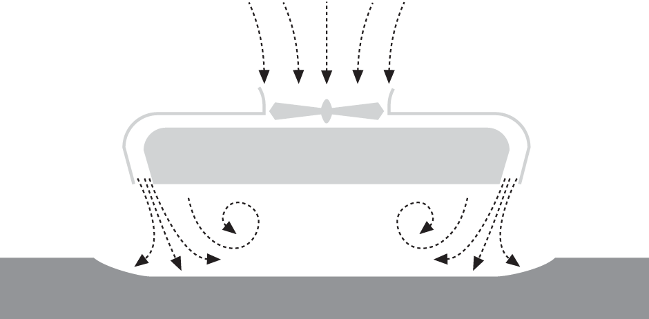
When a hovercraft operates over water, its air cushion creates a depression in the water surface due to cushion pressure (see Figure 17-4). At zero to low speeds, the weight of this displaced volume of water is equal to the weight of the craft, just as if the craft were floating in the water supported by buoyancy. As the craft starts to move forward, it tends to pitch up by the bow. When that happens, the surface of the water in the depressed region is approximately parallel to the bottom of the craft. As speed increases, the depression is reduced and the pitch angle tends to decrease.
Wave drag is a result of this depression and is equal to the horizontal components of pressure forces acting on the water surface in the depressed region. As it turns out, for small pitch angles and at low speeds, wave drag is on the same order of magnitude as the induced drag:
| Rwave ≈ W (tan τ) |
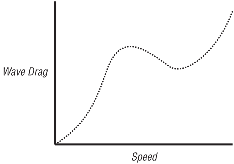
Since wave drag is proportional to the size of the depression, it tends to be highest at low speeds and decreases at higher operational speeds. If you were to plot the wave drag curve as a function of speed for a typical hovercraft, you’d find that it is not a straight or even parabolic curve, but rather it has a hump in the curve at the lower speed range, as illustrated in Figure 17-5.
There are several theoretical treatments of wave drag in the
literature that aim to predict the speed at which this hump occurs along
with its magnitude. These theories indicate that the hump depends on the
planform geometry of the hovercraft, and it tends to occur at speeds in
the range of ![]() to
to ![]() , where g is the acceleration due to
gravity and L is the length of the air cushion. In
practice, the characteristics of a particular hovercraft’s wave drag are
usually best determined through scale model testing.
, where g is the acceleration due to
gravity and L is the length of the air cushion. In
practice, the characteristics of a particular hovercraft’s wave drag are
usually best determined through scale model testing.
The so-called wetted drag is a function of several things:
The fact that parts of the hull and skirt tend to hit the water surface during flight
The impact of spray on the hull and skirt
The increase in weight as the hovercraft gets wet and sometimes takes on water
Wetted drag is difficult to predict, and in practice model tests are relied on to determine its magnitude for a particular design. It’s important to note, however, that this tends to be a significant drag component, sometimes accounting for as much as 30% of the total drag force.
Steering
In Chapter 9, the hovercraft was steered using a bow thruster that pushed transversely forward of the center of gravity. In reality, most hovercraft are steered by vectoring the thrust of the propulsion fan via rudders attached directly aft of the fans. This can be modeled by angling the propulsive thrust.
The most important characteristic to remember about steering hovercraft is that they will not turn like a car or boat. The hovercraft, because it has lower friction with its environment, will take longer to turn and tends to continue in the direction it was heading while rotating. Once rotated, the thrust acts along a new vector. One possible maneuver in a hovercraft is to quickly rotate the vessel and then shut down the propulsive thrust. This would allow you to travel in one direction and point in another for as long as your momentum carries you. This could be very useful in strafing enemies or just racking up style points.