
Chapter 5. Collisions
Now that you understand the motion of particles and rigid bodies, you need to consider what happens when they run into each other. That’s what we’ll address in this chapter; specifically, we’ll show you how to handle particle and, more interestingly, rigid-body collision response.
Before moving forward, we need to make a distinction between collision detection and collision response. Collision detection is a computational geometry problem involving the determination of whether and where two or more objects have collided. Collision response is a kinetics problem involving the motion of two or more objects after they have collided. While the two problems are intimately related, we’ll focus solely on the problem of collision response in this chapter. Later, in Chapter 7 through Chapter 13, we’ll show you how to implement collision detection and response in various real-time simulations, which draw upon concepts presented in this chapter.
Our treatment of rigid-body collision response in this chapter is based on classical (Newtonian) impact principles. Here, colliding bodies are treated as rigid irrespective of their construction and material. As in earlier chapters, the rigid bodies discussed here do not change shape even upon impact. This, of course, is an idealization. You know from your everyday experience that when objects collide they dent, bend, compress, or crumple. For example, when a baseball strikes a bat, it may compress as much as three-quarters of an inch during the millisecond of impact. Notwithstanding this reality, we’ll rely on well-established analytical and empirical methods to approximate rigid-body collisions.
This classical approach is widely used in engineering machine design, analysis, and simulations; however, for rigid-body simulations there is another class of methods, known as penalty methods, at your disposal.[13] In penalty methods, the force at impact is represented by a temporary spring that gets compressed between the objects at the point of impact. This spring compresses over a very short time and applies equal and opposite forces to the colliding bodies to simulate collision response. Proponents of this method say it has the advantage of ease of implementation. However, one of the difficulties encountered in its implementation is numerical instability. There are other arguments for and against the use of penalty methods, but we won’t get into the debate here. Instead, we’ve included several references in the Bibliography for you to review if you are so inclined. Other methods of modeling collisions exist as well. For example, nonlinear finite element simulations are commonly used to model collisions during product design, such as the impact of a cellphone with the ground. These methods can be quite accurate; however, they are too slow for real-time applications. Further, they are overkill for games.
Impulse-Momentum Principle
Impulse is defined as a force that acts over a very short period of time. For example, the force exerted on a bullet when fired from a gun is an impulse force. The collision forces between two colliding objects are impulse forces, as when you kick a football or hit a baseball with a bat.
More specifically, impulse is a vector quantity equal to the change in momentum. The so-called impulse-momentum principle says that the change in moment is equal to the applied impulse. For problems involving constant mass and moment of inertia, you can write:
| Linear impulse = ȫ (t– to t+) F dt = m (v+ – v–) |
| Angular impulse = ȫ (t– to t+) M dt = I (ω+ – ω–) |
In these equations, F is the impulsive force, M is the impulsive torque (or moment), t is time, v is velocity, the subscript – refers to the instant just prior to impact, and the subscript + refers to the instant just after impact. You can calculate the average impulse force and torque using the following equations:
| F = m (v+ – v–) / (t+ – t–) |
| M = I (ω+ – ω–) / (t+ – t–) |
Consider this simple example: a 150 gram (0.15 kg) bullet is fired from a gun at a muzzle velocity of 756 m/s. The bullet takes 0.0008 seconds to travel through the 610 mm (0.610 m) rifle barrel. Calculate the impulse and the average impulsive force exerted on the bullet. In this example, the bullet’s mass is a constant 150 grams and its initial velocity is 0, thus its initial momentum is 0. Immediately after the gun is fired, the bullet’s momentum is its mass times the muzzle velocity, which yields a momentum of 113.4 kg-m/s. The impulse is equal to the change in momentum, and is simply 113.4 kg-m/s. The average impulse force is equal to the impulse divided by the duration of application of the force, or in this case:
| Average impulse force = (113.4 kg-m/s) / (0.0008 s) |
| Average impulse force = 141,750 N |
This is a simple but important illustration of the concept of impulse, and you’ll use the same principle when dealing with rigid-body impacts. During impacts, the forces of impact are usually very high and the duration of impact is usually very short. When two objects collide, each applies an impulse force to the other; these forces are equal in magnitude but opposite in direction. In the gun example, the impulse applied to the bullet to set it in motion is also applied in the opposite direction to the gun, giving you a nice kick in the shoulder. This is simply Newton’s third law in action.
Impact
In addition to the impulse momentum principle discussed in the previous section, our classical impact, or collision response, analysis relies on another fundamental principle: Newton’s principle of conservation of momentum, which states that when a system of rigid bodies collide, momentum is conserved. This means that for bodies of constant mass, the sum of their masses times their respective velocities before the impact is equal to the sum of their masses times their respective velocities after the impact:
| m1v1– + m2v2– = m1v1+ + m2v2+ |
Here, m refers to mass, v refers to velocity, subscript 1 refers to body one, subscript 2 refers to body two, subscript – refers to the instant just prior to impact, and subscript + refers to the instant just after impact.
A crucial assumption of this method is that during the instant of impact the only force that matters is the impact force; all other forces are assumed negligible over that very short duration. Remember this assumption, because in Chapter 10 we’ll rely on it when implementing collision response in an example 2D real-time simulation.
We’ve already stated that rigid bodies don’t change shape during impacts, and you know from your own experience that real objects do change shape during impacts. What’s happening in real life is that kinetic energy is being converted to strain energy to cause the objects to deform. (See the sidebar Kinetic Energy for further details on this topic.) When the deformation in the objects is permanent, energy is lost and thus kinetic energy is not conserved.
Collisions that involve losses in kinetic energy are said to be inelastic, or plastic, collisions. For example, if you throw two clay balls against each other, their kinetic energy is converted to permanent strain energy in deforming the clay balls, and their collision response—that is, their motion after impact—is less than spectacular. If the collision is perfectly inelastic, then the two balls of clay will stick to each other and move together at the same velocity after impact. Collisions where kinetic energy is conserved are called perfectly elastic. In these collisions, the sum of kinetic energy of all objects before the impact is equal to the sum of kinetic energy of all objects after the impact. A good example of elastic impact (though not perfectly elastic) is the collision between two billiard balls where the ball deformation is negligible and certainly not permanent under normal circumstances.
Of course, in reality, impacts are somewhere between perfectly elastic and perfectly inelastic. This means that for rigid bodies, which don’t change shape at all, we’ll have to rely on an empirical relation to quantify the degree of elasticity of the impact(s) that we’re trying to simulate. The relation that we’ll use is the ratio of the relative separation velocity to the relative approach velocity of the colliding objects:
| e = −(v1+ − v2+) / (v1− − v2−) |
Here e is known as the coefficient of restitution and is a function of the colliding objects’ material, construction, and geometry. This coefficient can be experimentally determined for specific impact scenarios—for example, the collision between a baseball and bat, or a golf club and ball. For perfectly inelastic collisions, e is 0, and for perfectly elastic collisions, e is 1. For collisions that are neither perfectly inelastic nor perfectly elastic, e can be any value between 0 and 1. In this regard, the velocities considered are along the line of action of the collision.
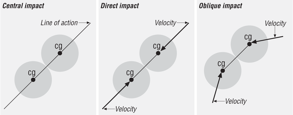
In frictionless collisions, the line of action of impact is a line perpendicular (or normal) to the colliding surfaces. When the velocity of the bodies is along the line of action, the impact is said to be direct. When the line of action passes through the center of mass of the bodies, the collision is said to be central. Particles and spheres of uniform mass distribution always experience central impact. Direct central impact occurs when the line of action passes through the centers of mass of the colliding bodies and their velocity is along the line of action. When the velocities of the bodies are not along the line of action, the impact is said to be oblique. You can analyze oblique impacts in terms of component coordinates where the component parallel to the line of action experiences the impact, but the component perpendicular to the line of action does not. Figure 5-1 illustrates these impacts.
As an example, consider the collision between two billiard balls illustrated in Figure 5-2.
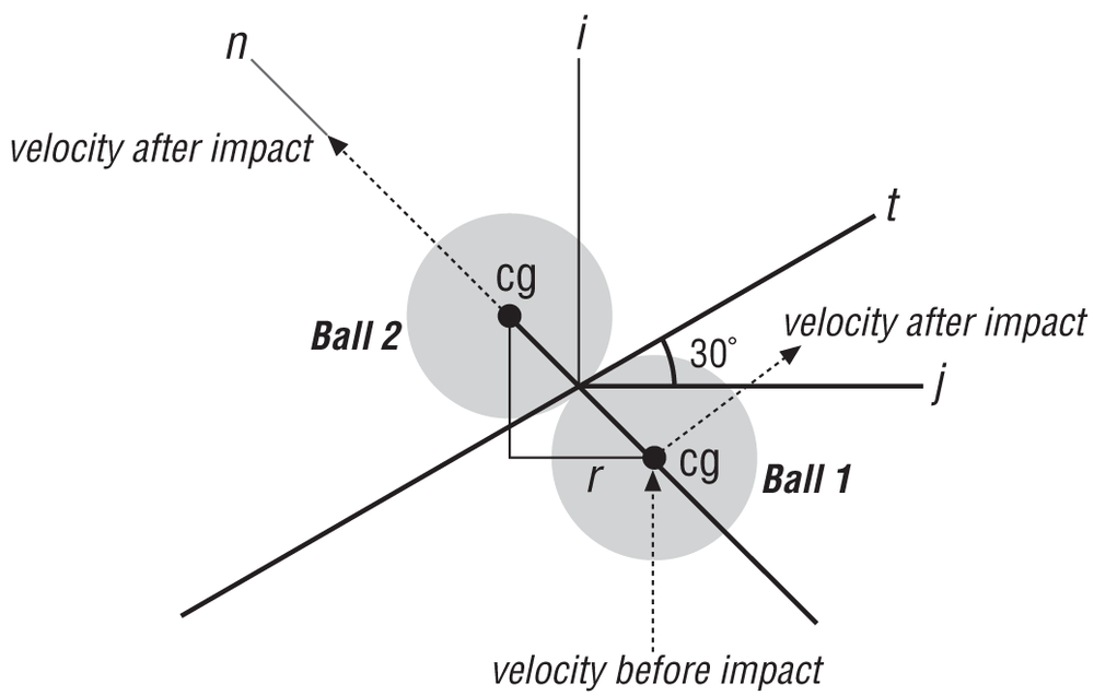
Both balls are a standard 57 mm in diameter, and each weighs 156 grams. Assume that the collision is nearly perfectly elastic and the coefficient of restitution is 0.9. If the velocity of ball 1 when it strikes ball 2 is 6 m/s in the x-direction, as shown in Figure 5-2, calculate the velocities of both balls after the collision assuming that this is a frictionless collision.
The first thing you need to do is recognize that the line of action of impact is along the line connecting the centers of gravity of both balls, which, since these are spheres, is also normal to both surfaces. You can then write the unit normal vector as follows:
| n = |
| n = (0.866) i – (0.5)j |
where n is the unit normal vector, r is the ball radius, and i and j represent unit vectors in the x- and y-directions, respectively.
Now that you have the line of action of the collision, or the unit normal vector, you can calculate the relative normal velocity between the balls at the instant of collision.
| vrn = [v1– – v2–] • n |
| vrn = [(6 m/s) i + (0 m/s) j ] • [ (0.864) i – (0.5) j] |
| vrn = 5.18 m/s |
This will be used as v1n– in the following equations. Notice here that since ball 2 is initially at rest, v2– is 0.
Now you can apply the principle of conservation of momentum in the normal direction as follows:
| m1 v1n– + m2 v2n– = m1 v1n+ + m2 v2n+ |
Noting that m1 equals m2 since the balls are identical, and that v2n– is 0, and then solving for v1n+ yields:
| v1n+ = v1n– – v2n+ |
To actually solve for these velocities, you need to use the equation for coefficient of restitution and make the substitution for v1n+. Then, you’ll be able to solve for v2n+. Here’s how to proceed:
| e = (–v1n+ + v2n+) / (v1n– – v2n–) |
| e v1n– = –(v1n– – v2n+) + v2n+ |
| v2n+ = v1n– (e + 1) / 2 |
| v2n+ = (5.18 m/s)(1.9) / 2 = 4.92 m/s |
Using this result and the formula for v1n+ yields:
| v1n+ = 5.18 m/s – 4.92 m/s = 0.26 m/s |
Since the collision is frictionless, there is no impulse acting in the tangential direction. This means that momentum is conserved in that direction too and that the final tangential speed of ball 1 is equal to its initial tangential speed, which in this case is equal to 3 m/s (this equals (6m/s) sin 30°). Since ball 2 had no initial tangential speed, its velocity after impact is solely in the normal direction. Converting these results back to x-y coordinates instead of normal and tangential coordinates yields the following velocities for each ball after impact:
| v2+ = (4.92 m/s) sin 60° i – (4.92 m/s) cos 60 ° j |
| v1+ = [(0.26 m/s) cos 30° + (3 m/s) sin 30°] i + |
| + [(−0.26 m/s) sin 30° + (3 m/s) cos 30°)] j |
| v1+ = (1.72 m/s) i + (2.47 m/s) j |
To further illustrate the application of these collision response principles, consider another example, this time the collision between a baseball bat and baseball (as shown in Figure 5-3). We are looking at a side view, staring down the barrel of the bat.
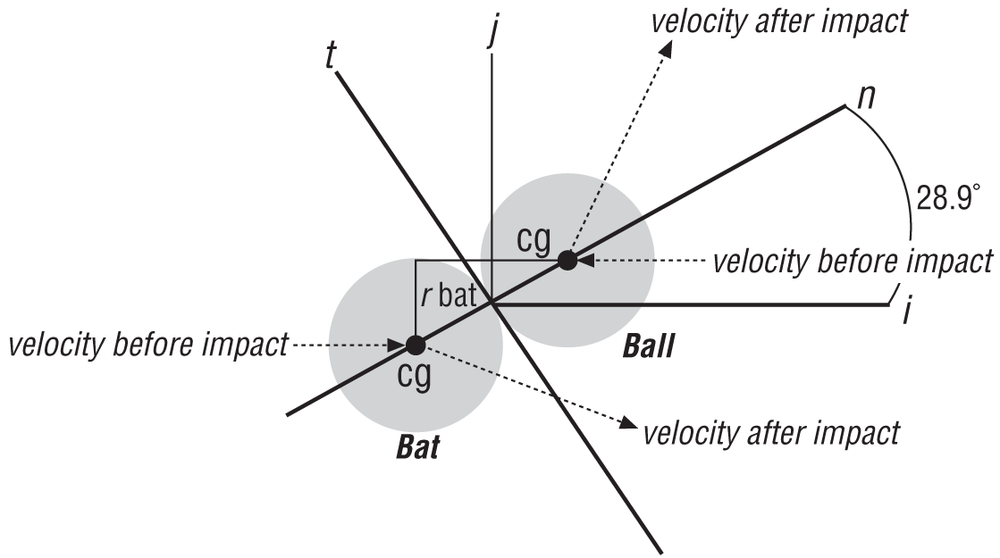
To a reasonable degree of accuracy, the motion of a baseball bat at the instant of collision can generally be described as independent of the batter—in other words, you can assume that the bat is moving freely and pivoting about a point located near the handle end of the bat. Assume that the ball strikes the bat on the sweet spot—that is, a point near the center of percussion.[14] Further assume that the bat is swung in the horizontal plane and that the baseball is traveling in the horizontal plane when it strikes the bat. The bat is of standard dimensions with a maximum diameter of 70 mm and a weight of 1.02 kg. The ball is also of standard dimensions with a radius of 37 mm and a weight of 0.15 kg. The ball reaches a speed of 40 m/s (90 mph) at the instant it strikes the bat, and the speed of the bat at the point of impact is 31 m/s (70 mph). For this collision, the coefficient of restitution is 0.46. In the millisecond of impact that occurs, the baseball compresses quite a bit; however, in this analysis assume that both the bat and the ball are rigid. Finally, assume that this impact is frictionless.
As in the previous example, the line of action of impact is along the line connecting the centers of gravity of the bat and ball; thus, the unit normal vector is:
| n = |
| n = (0.875) i + (0.484) j |
Here the subscripts 1 and 2 denote the bat and ball, respectively.
The relative normal velocity between the bat and ball is:
| vrn = [v1− − v2−] • n |
| vrn = [(71 m/s) i + (0 m/s) j ] • [ (0.875) i − (0.484) j] |
| vrn = 62.1 m/s |
The velocity components of the bat and ball in the normal direction are:
| v1n− = v1− • n = 27.1 m/s |
| v2n− = v2− • n = −35.0 m/s |
Applying the principle of conservation of momentum in the normal direction and solving for v1n+ yields:
| m1 v1n− + m2 v2n− = m1 v1n+ + m2 v2n+ |
| (1.02 kg) (27.1 m/s) + (0.15 kg) (−35.2 m/s) = |
| =(1.02 kg) v1n+ + (0.15 kg) v2n+ |
| v1n+ = 21.92 m/s − (0.14 m/s) v2n+ |
As in the previous example, applying the formula for coefficient of restitution with the preceding formula for v1n+ yields:
| e = (−v1n+ + v2n+) / (v1n− − v2n−) |
| 0.46 = [−21.92 m/s + (0.14 m/s) v2n+ + v2n+] / [27.1 m/s + 35.2 m/s] |
| v2n+ = 44.4 m/s and v1n+ = 15.7 m/s |
Here again, since this impact is frictionless, each object retains its original tangential velocity component. For the bat, this component is 15 m/s, while for the ball it’s −19.3 m/s. Converting these normal and tangential components to x-y coordinates yields the following bat and ball velocities for the instant just after impact:
| v1+ = 21.0 m/s i − 5.5 m/s j |
| v2+ = 30 m/s i + 38.7 m/s j |
Both of these examples illustrate fundamental impact analysis using the classical approach. They also share an important assumption—that the impacts are frictionless. In reality, you know that billiard balls and baseballs and bats collide with friction; otherwise, you would not be able to apply English in billiards or create lift-generating spin on baseballs. Later in this chapter we’ll discuss how to include friction in your impact analysis.
Linear and Angular Impulse
In the previous section, you were able to work through the specific examples by hand using the principle of conservation of momentum and the coefficient of restitution. This approach will suffice if you’re writing games where the collision events are well defined and anticipated. However, if you’re writing a real-time simulation where objects, especially arbitrarily shaped rigid bodies, may or may not collide, then you’ll want to use a more general approach. This approach involves the use of formulas to calculate the actual impulse between colliding objects so that you can apply this impulse to each object, instantly changing its velocity. In this section, we’ll derive the equations for impulse, both linear and angular, and we’ll show you how to implement these equations in code in Chapter 10.
When you’re dealing with particles or spheres, the only impulse formula that you’ll need is that for linear impulse, which will allow you to calculate the new linear velocities of the objects after impact. So, the first formula that we’ll derive for you is that for linear impulse between two colliding objects, as shown in Figure 5-4.
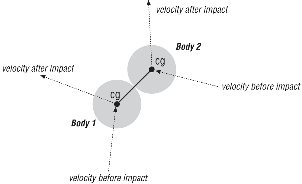
For now, assume the collision is frictionless and the line of action of the impulse is along the line connecting the centers of mass of the two objects. This line is normal to the surfaces of both objects.
To derive the formula for linear impulse, you have to consider the formula from the definition of impulse along with the formula for coefficient of restitution. Here let J represent the impulse:
| |J| = m (|v+| − |v−|) |
| e = −(|v1+| − |v2+|)/(|v1−| − |v2−|) |
In these equations the velocities are those along the line of action of the impact, which in this case is a line connecting the centers of mass of the two objects. Since the same impulse applies to each object (just in opposite directions), you actually have three equations to deal with:
| |J| = m1 (|v1+| − |v1−|) |
| |−J| = m2 (|v2+| − |v2−|) |
| e = −(|v1+|− |v2+|)/(|v1−| − |v2-|) |
Notice we’ve assumed that J acts positively on body 1 and its negation, –J, acts on body 2. Also notice that there are three unknowns in these equations: the impulse and the velocities of both bodies after the impact. Since there are three equations and three unknowns, you can solve for each unknown by rearranging the two impulse equations and substituting them into the equation for e. After some algebra, you’ll end up with a formula for J that you can then use to determine the velocities of each body just after impact. Here’s how that’s done:
| For body 1: |v1+| = |J|/m1 + |v1–| |
| For body 2: |v2+| = –|J|/m2 + |v2–| |
Substituting |v1+| and |v2+| into the equation for e yields:
| e (|v1–| – |v2–|) = –[( |J|/m1 + |v1–|) – (–|J|/m2 + |v2–|)] |
| e (|v1-| – |v2–|) + |v1–| – |v2–| = –J (1/m1 + 1/m2) |
Let |vr| = (|v1–| – |v2–|); then:
| e |vr| + |vr| = –|J| (1/m1 + 1/m2) |
| |J| = –|vr|(e + 1)/(1/m1 + 1/m2) |
Since the line of action is normal to the colliding surfaces, vr is the relative velocity along the line of action of impact, and J acts along the line of action of impact, which in this case is normal to the surfaces, as we’ve already stated.
Now that you have a formula for the impulse, you can use the definition of impulse along with this formula to calculate the change in linear velocity of the objects involved in the impact. Here’s how that’s done in the case of two objects colliding:
| v1+ = v1– + (|J| n)/m1 |
| v2+ = v2– + (–|J| n)/m2 |
Notice that for the second object, the negative of the impulse is applied since it acts on both objects equally but in opposite directions.
When dealing with rigid bodies that rotate, you’ll have to derive a new equation for impulse that includes angular effects. You’ll use this impulse to calculate new linear and angular velocities of the objects just after impact. Consider the two objects colliding at point P, as shown in Figure 5-5.
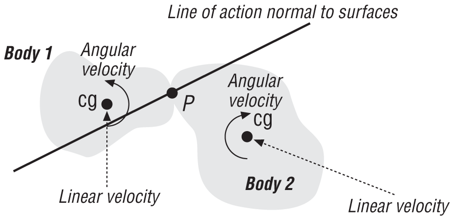
There’s a crucial distinction between this collision and that discussed earlier. In this case, the velocity at the point of contact on each body is a function of not only the objects’ linear velocity but also their angular velocities, and you’ll have to recall from Chapter 2 the following formula in order to calculate the velocities at the impact point on each body:
| vp = vg + (ω × r) |
In this relation, r is the vector from the body’s center of gravity to the point P.
Using this formula, you can rewrite the two formulas relating the linear velocity after impact to the impulse and initial velocity as follows:
| For body 1: v1g+ + (ω1+ × r1) = J/m1 + v1g– + (ω1– × r1) |
| For body 2: v2g+ + (ω2+ × r2) = –J/m2 + v2g– + (ω2– × r2) |
There are two additional unknowns here, the angular velocities after impact, which means that you need two additional equations. You can get these equations from the definition of angular impulse:
| For body 1: (r1 × J) = I1 (ω1+ – ω1–) |
| For body 2: (r2 × –J) = I2 (ω2+ – ω2–) |
Here we calculate the moment due to the impulse by taking the vector cross product of the impulse with the distance from the body’s center of gravity to the point of application of the impulse.
By combining all of these equations with the equation for e and following the same procedure used when deriving the linear impulse formula, you’ll end up with a formula for |J| that takes into account both linear and angular effects, which you can then use to find the linear and angular velocities of each body immediately after impact. Here’s the result:
| |J| = –(vr• n)(e + 1)/[1/m1 + 1/m2 + n •((r1 × n)/I1) × r1 + n • ((r2 × n)/I2) × r2] |
Here vr is the relative velocity along the line of action at the impact point P, and n is a unit vector along the line of action at the impact point pointing out from body 1.
With this new formula for |J|, you can calculate the change in linear and angular velocities of the objects involved in the collision using these formulas:
| v1+ = v1− + (|J| n)/m1 |
| v2+ = v2− + (−|J| n)/m2 |
| ω1+ = ω1− + (r1 × |J| n)/I1 |
| ω2+ = ω2− + (r2 × −|J| n)/I2 |
As we said earlier, we’ll show you how to implement these formulas for impulse in code when you get to Chapter 10.
Friction
Friction acts between contacting surfaces to resist motion. When objects collide in any type of collision except direct impact, for that very brief moment of contact, they will experience a friction force that acts tangentially to the contacting surfaces. Not only will this tangential force change the linear velocities of the colliding objects in the tangential direction, but it will also create a moment (torque) on the objects, which tends to change their angular velocities. This tangential impulse combined with the normal impulse results in an effective line of action of the total collision impulse that is no longer perpendicular to the contacting surfaces.
In practice, it is very difficult to quantify this collision friction force due to the fact that the friction force is not necessarily constant if the collision is such that the friction force does not develop beyond the maximum static friction force. Further complications stem from the fact that objects do tend to deform when they collide, creating an additional source of resistance. That said, since the friction force is a function of the normal force between the contacting surfaces, you know that the ratio of the normal force to the friction force is equal to the coefficient of friction. If you assume that the collisions are such that the kinetic coefficient of friction is applicable, then this ratio is constant.
| µk = Ff / Fn |
Here, Ff is the tangential friction force and Fn is the normal impact force. You can extend this to say that the ratio of the tangential impulse to normal impulse is equal to the coefficient of friction.
Consider the collision between the golf club head and golf ball illustrated in Figure 5-6.
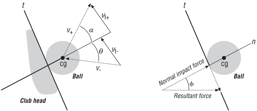
In the upper velocity diagram, v– represents the relative velocity between the ball and club head at the instant of impact, v+ represents the velocity of the ball just after impact, vt– and vt+ represent the tangential components of the ball velocity at and just after the instant of impact, respectively.
If this were a frictionless collision, vt– and vt+ would be equal, as would the angles α and θ. However, with friction the tangential velocity of the ball is reduced, making vt+ less than vt–, which also means that α will be less than θ.
The lower force diagram in Figure 5-6 illustrates the forces involved in this collision with friction. Since the ratio of the tangential friction force to the normal collision force is equal to the coefficient of friction, you can develop an equation relating the angle φ to the coefficient of friction.
| tan φ = Ff / Fn = µ |
In addition to this friction force changing the linear velocity of the ball in the tangential direction, it will also change the angular velocity of the ball. Since the friction force is acting on the ball’s surface some distance from its center of gravity, it creates a moment (torque) about the ball’s center of gravity, which causes the ball to spin. You can develop an equation for the new angular velocity of the ball in terms of the normal impact force or impulse:
| Σ Mcg = Ff r = Icg dω/dt |
| µ Fn r = Icg dω/dt |
| µ Fn r dt = Icg dω |
| ȫ(t– to t+) Fn dt = Icg / (µ r) ȫ(ω– to ω+) ω dω |
Notice here that the integral on the left is the normal impulse; thus:
| Impulse = Icg / (µ r) (ω+ – ω–) |
| ω+ = (Impulse) (µ r) / Icg + ω– |
This relation looks very similar to the angular impulse equation that we showed you earlier in this chapter, and you can use it to approximate the friction-induced spin in specific collision problems.
Turn back to the equation for impulse, J, in the last section that includes both linear and angular effects. Here it is again for convenience:
| |J| = –(vr• n)(e + 1) / [1/m1 + 1/m2 + n •((r1 × n)/I1) × r1 + n • ((r2 × n)/I2) × r2] |
This formula gives you the collision impulse in the normal direction. To see how friction fits in you must keep in mind that friction acts tangentially to the contacting surfaces, that combining the friction force with the normal impact force yields a new effective line of action for the collision, and that the friction force (and impulse) is a function of the normal force (impulse) and coefficient of friction. Considering all these factors, the new equations to calculate the change in linear and angular velocities of two colliding objects are as follows:
| v1+ = v1– + (J n + (µ J) t) / m1 |
| v2+ = v2– + (–J n + (µ J) t) / m2 |
| ω1+ = ω1– + (r1 × (J n+ (µ J) t)) / Icg |
| ω2+ = ω2– + (r2 × (–J n+ (µ J) t)) / Icg |
In these equations, t is the unit tangent vector, which is tangent to the collision surfaces and at a right angle to the unit normal vector. You can calculate the tangent vector if you know the unit normal vector and the relative velocity vector in the same plane as the normal vector.
| t = (n × vr) × n |
| t = t / |t| |
For many problems that you’ll face, you may be able to reasonably neglect friction in your collision response routines since its effect may be small compared to the effect of the normal impulse itself. However, for some types of problems, friction is crucial. For example, the flight trajectory of a golf ball depends greatly on the spin imparted to it as a result of the club–ball collision. We’ll discuss how spin affects trajectory in the next chapter, which covers projectile motion.
[13] We use the classical approach in this book and are mentioning penalty methods only to let you know that the method we’re going to show is not the only one. Roughly speaking, the penalty in penalty methods refers to the numerical spring constants, which are usually large, that are used to represent the stiffness of the springs and thus the hardness (or softness) of the colliding bodies. These constants are used in the system of equations of motion describing the motion of all the bodies under consideration before and after the collision.
[14] The center of percussion is a point located near one of the nodes of natural vibration, and is the point at which, when the bat strikes the ball, no force is transmitted to the handle of the bat. If you’ve ever hit a baseball incorrectly such that you get a painful vibrating sensation in your hands, then you know what it feels like to miss the center of percussion.