
After going over some specialized distributions of Linux for the Tinker Board, it’s time to return to where this book began: TinkerOS. This time around, we’re going to be applying the Linux, GPIO, and programming skills that we gained in the first part of the book. The first project that we’ll tackle is an Internet-connected display with an e-Paper module that will show the current date, time, and weather.
What Is e-Paper?
Often referred to as e-Ink or EPD , e-Paper (electronic paper) is a digital display that mimics the look of ink on paper. It’s the same type of display found in e-readers and other similar devices. It has a slow refresh rate, so it’s best for static displays, such as images or slowly changing text. Because of this, it has incredibly low power consumption. e-Paper is also known for being easily visible in all lighting conditions, including direct sunlight, and it’s easier on your eyes because it doesn’t emit the blue light found in LCD displays.
e-Paper comes in a variety of shapes and sizes. Traditionally, the displays are dual-color; usually black and white, but newer versions can showcase other colors, and tricolor displays are also beginning to come to market. They’re becoming increasingly popular for DIY applications, since they’re available for multiple platforms. Many displays can be coded in multiple coding languages with manufacturer-provided libraries that you can install, along with example code to test included. They usually connect through individual broken-out pins to attach to GPIO pins on different boards, but there are also specialized add-on boards that fit directly onto certain boards’ GPIO layouts, including the Tinker Board.
The display that we’re going to use for this project is from Waveshare , a manufacturer of DIY electronics accessories. They have quite a few varieties of e-Paper displays available, and the one we’ll be looking at is the 2.13-inch HAT variety. It was originally designed to work with Raspberry Pi, but ASUS has ported the Python libraries to work with the Tinker Board so that no code adjustment is needed. We’ll examine what they did, though, so that you can try porting hardware libraries for future projects.
SPI
You may be wondering how the e-Paper displays work. Some, including the one we’ll be using, use Serial Peripheral Interface (SPI) communication . SPI is a bus protocol used to communicate between devices. It has a built-in clock signal that is sent in conjunction with any data for highly accurate and timely communication. SPI is integrated into Python using the spidev library, which we’ll discuss shortly as we prepare for the Waveshare library installation.
Early Issues with SPI on the Tinker Board
Previously, there were some issues with SPI on the Tinker Board. Although both the original Tinker Board and Tinker Board S have two SPI controllers, SPI0 and SPI2, available via the GPIO, only SPI2 was enabled at the kernel level. Beginning with TinkerOS 2.0.7, this issue has been resolved and now both SPI0 and SPI2 can be utilized. This increases compatibility with a lot of hardware.

The nano text file for I2C and SPI settings
The e-Paper Display’s Hardware
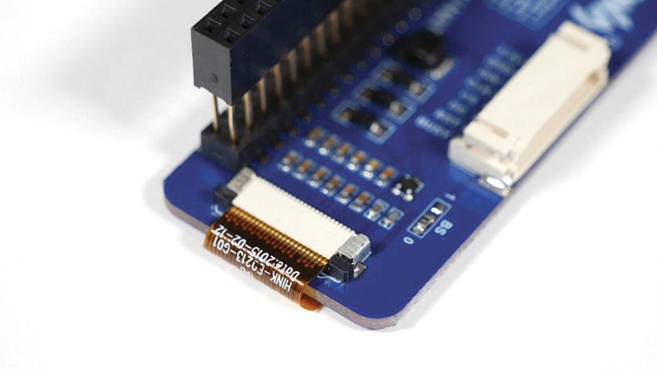
The EPD’s ribbon cable that connects to the HAT
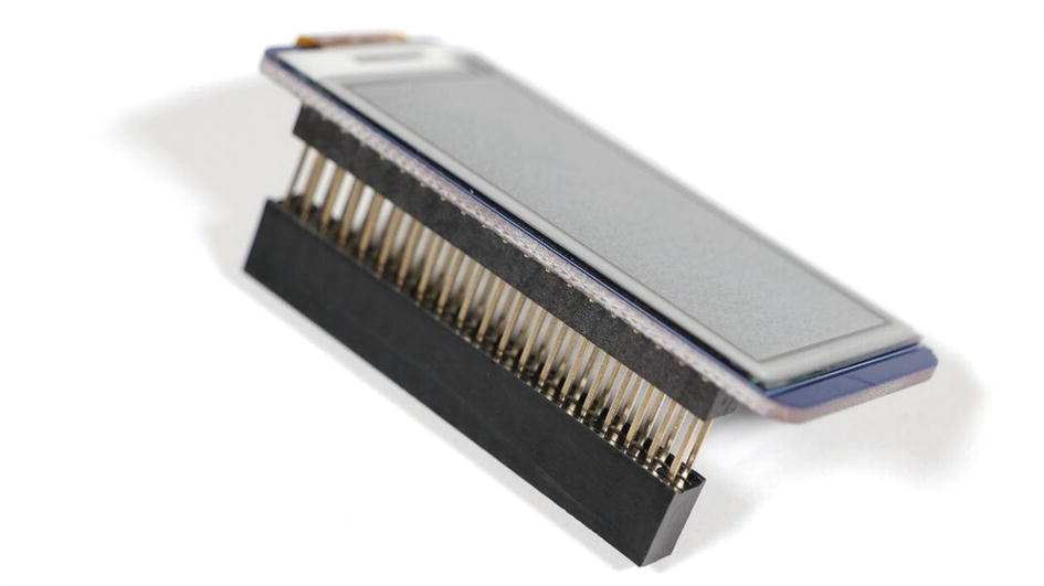
The 40-pin header being used as a riser for the 2.13-inch EPD HAT
Setting Up the EPD’s Software
As mentioned previously, we’re going to use the EPD with TinkerOS. Boot into TinkerOS and then navigate to the terminal so that we can begin installing the Python dependencies.
pip is a package management system that allows you to install Python dependencies, tools and libraries for Python, similar to using apt-get install or git for other programs and downloads in Linux. However, best results for installation occur when you’re targeting the Home directory. Using pip, we’re going to install the SPI library by entering pip install spidev into the terminal. After that, run sudo apt-get upgrade and sudo reboot.
Note
Some dependencies, like python-dev , were installed during other chapters. They’re repeated here in case you didn’t follow directly along with those chapters. Trying to install them again won’t damage your build of TinkerOS; they’ll just be ignored.
The 7zip file hosted on the Tinker Board wiki site for Waveshare add-ons. It’s located at the very bottom of the web page, which is linked in Footnote 1.
You can download and unzip the folder either on your main computer or on the Tinker Board. If you access it with the Tinker Board, best results for unzipping were experienced using the GUI tools rather than the terminal since it’s a 7zip folder rather than a zip folder. Once you open the folder, you’ll see files labeled epd2in13.py, epdif.py, main.py, and monocolor.bmp. The epd2in13.py and epdif.py files are the library files. You’ll need to have these files in the same folder as your Python program for the display so that it runs properly. The main.py file is a demo program for the display, and monocolor.bmp is a bitmap picture formatted to appear properly on the display. The main.py program has some lines of code that call for this bitmap to be displayed.
Ported Libraries
Before we see the final result of these ported libraries, let’s see what makes them tick. Studying these will also help in understanding how to get started with porting code and libraries to the Tinker Board later.
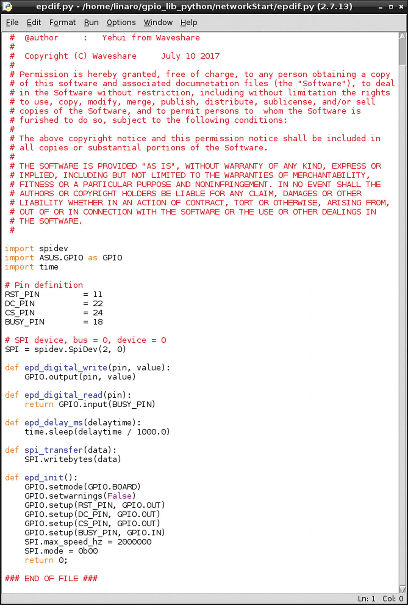
The epdif.py file. You can reference this figure for the entire discussion of the epdif.py file.
Looking further, we can also see that the spidev library is being imported here, which implies that SPI settings along with GPIO settings will be taken care of with this file. Sure enough, the next section of code defines the pins needed from the GPIO for SPI. Pins for Reset, DC (Data/Command control), CS (SPI chip select), and Busy (Busy state output) for the e-Paper display are assigned to the proper Tinker Board physical board pins. This is another item you’ll want to check, since many Raspberry Pi libraries utilize a different numbering convention.
Next, we see SPI being set up to run with the SPI2 bus by calling spidev.SpiDev(2, 0). If you wanted to change this to run on SPI0, you’d call spidev.SpiDev(0, 0).
Following SPI, we have some digital_write and digital_read functions for the GPIO pins that were previously defined. But the most notable and important function is epd.init() , which will be called for most major commands with the e-Paper display. It basically finishes setting up the GPIO pins and then resets them to their default states. You can see the call for the GPIO.Board numbering convention, followed by code that sets Reset, DC, and CS as outputs and Busy as an input. You can also see that the SPI speed and mode are defined as well. Later, when you see epd.init() called, know that this process is happening along with the other parameter that will be inside the parentheses.
Technically these functions and definitions could be written in your main code, but it would make your code very long, possibly create conflicts, and slow things down. The purpose of libraries and dependency files is to take care of a lot of the back-end prep aspects of code so that it can simply be referenced in the main code file.
The Second Library File
After finishing up with epdif.py, we can look at the second and final library file, ep2in13.py , by entering idle ep2in13.py into the terminal. The name refers to the official name of the EPD and contains a lot of driver communication for the display.

The top of the ep2in13.py file
The other major adjustable item is the screen resolution, defined directly under the library imports. The resolution for this display is set to 128 pixels wide and 250 pixels high. This means that the driver and library consider this to be a vertical display. We’ll want to change the display to show horizontally for our project, but we’ll take care of that in our main code rather than here, since the driver and other library dependencies are written with a vertical orientation in mind.
The rest of the file contains the library commands and functions that make it easier to communicate succinctly with the display, some of which we’ll see shortly in the demo code. You can also reference this file to see if there are any additional functions that will be beneficial to your code or to create your own functions. Many of these will be nested in the epd.init() function as well.
Demo Code
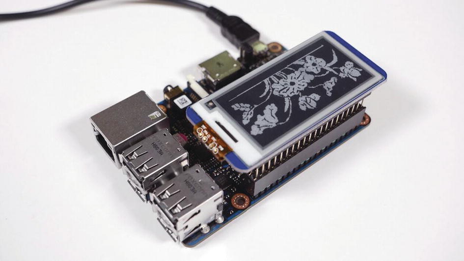
The bitmap file showing on the EPD HAT while the included demo code runs
Running the demo code should give you an idea of what these displays are capable of. Knowing what’s included in the libraries now, let’s take a closer look at main.py to understand how the program code is structured and how we’ll be able to write our own code for our display project.
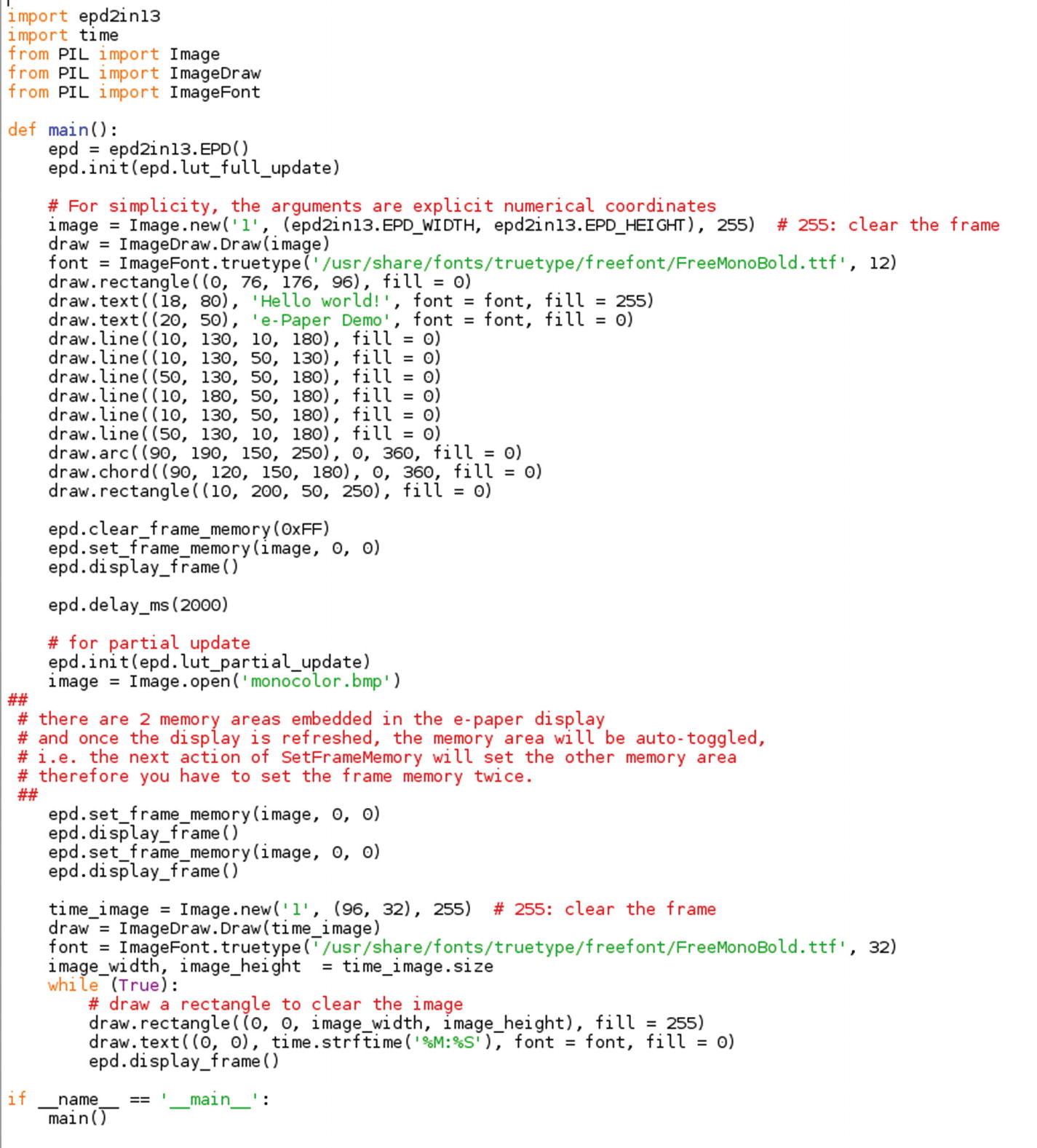
The main.py demo code file
The PIL library was mentioned briefly when we saw it imported in the ep2in13.py file. PIL is the Python Imaging Library. It’s an image-processing library that allows you to manipulate images in a variety of ways, including editing pixels with the ImageDraw portion of the library. The current form of PIL is actually a fork of the original library called Pillow2 and is widely used in a variety of applications. Beyond the hardware and SPI communication, it’s basically the backbone of the EPD since it allows for the hard-coded images and imported image files to be displayed and controlled.
Then we move on to main(), where the bulk of the code lives. First, epd is defined as epd2in13.EPD(), referring to the library file, and then the display is initialized with a full update by calling epd.init(epd.lut_full_update), which results in the screen flashing black and white a few times when starting main.py.

The lines of code that create the first image drawn for the demo code
The first three lines in this block of code define image, draw, and font, which will be called throughout the script. The image parameter is used to refer to everything drawn on the display. For example, if you program three circles and a word to appear together, it is defined as an image and is created by calling image.new. The other parameters defined here are the size of the image (usually matching the resolution listed in the library, as we saw in epd2in13.py) and the color, which is expressed as a number. Here it’s entered as 255, which is white. For this library, 0 will mean black and 255 will mean white. When setting up an image, always call 255 so that the frame can be cleared as commented in the code.
The draw method is called to “draw” the image. By “drawing,” it’s sending data to the screen as interpreted from all the parameters that are called later in conjunction with draw.object() . Finally, font is used to pull a font library from a file directory in TinkerOS to be used for drawing strings. For each font that you use you’ll need to create a new font object. The font size is also defined after the file directory position, as shown in Figure 10-9.
The remaining lines in the block are the items that appear on the screen, programmed one item at a time using draw.rectangle, draw.text, draw.line, draw.arc, and draw.chord, which is a circle. For the shapes and lines, the four numbers in the parentheses are coordinates for their origin and end points using an (x, y, x, y) format. Since they are being “drawn,” you’re essentially telling the PIL library to send the pixels with the coordinates acting as a map. The fill parameter is for color, calling for a number between 0 and 255. The chord and arc shapes have an extra parameter for degrees in a range of 0 to 360.
text is set up a bit differently than the shapes. It only has one set of coordinates, which represent the starting point. This is followed by the string that will be written to the screen. Finally, the font is defined along with the fill color.
Note
Keep track of commas and parentheses when creating these items in your code. The syntax is very important and very particular.
The remainder of main() contains the more technical aspects of the code, controlling how the EPD properly shows the data. The first three commands, clear_frame_memory, set_frame_memory and display_frame() are called immediately after the image is written. The HAT has two memory banks to store the data that it receives from the Tinker Board, and they need to be manually cleared and refreshed. clear_frame_memory completely erases both memory banks and is called only once. set_frame_memory (image, 0, 0) is then called to send the image to the memory banks with 0, 0 acting as coordinates. The final command is display_frame() , which pushes the image from memory to the display.
After the image is pushed to the display, a delay is called with delay_ms(2000). It’s expressed in milliseconds, so the 2000 means 2 seconds. The delay’s purpose is essentially to set the refresh rate for the display, meaning that every 2 seconds the code will update the image by refreshing itself so that any changes enacted will be pushed to the display.
The next line begins this refresh process by calling epd.init(ped.lut_partial_update), which runs a partial update to the display. This happens to subtly refresh the pixels, unlike the rapid flashing of black and white that occurs with the full update called at the beginning of the script. This line sets the stage for a new image to be defined and then called with image.open('monocolor.bmp'), which opens the bitmap file that we’ve seen in the folder. By calling image.open, you can import image files that are in formats supported by PIL.
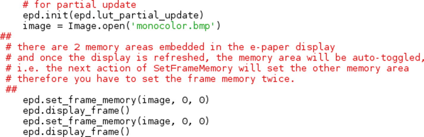
The set_frame_memory() commands after a new image is created
This time, set_frame_memory (image, 0, 0), with image referring to the newly imported bitmap, and display_frame() are both called twice. As mentioned previously, the EPD has two memory banks, and by calling both of those commands twice, we make sure each bank receives the new image to display and updates. If both of these were only called once, it would cause the display to be glitchy; and if they weren’t called at all, the display would not update. We didn’t need to call them twice when the original image was sent, because the memory had been fully cleared using clear_frame_memory .
The final portion of the code is possibly formatted incorrectly, depending on the intent of the developer. As you can see in Figure 10-11, an additional new image is created, this time called time_image . After the parameters for this new image are set, we enter a loop using while True: that will display a rectangle with some text meant for time_image. The text is formatted to be a digital clock using time.strftime('%M:%S'). Using strftime() from the time library allows you to display real-time time data, such as a date, or in this case a clock, using custom formatting with % signs and letters, as shown with ('%M:%S'). We’ll discuss this concept further when we write the code for our project.
Because we placed the time.strftime() in the loop, it will update rather than remaining static as it would when called outside the loop. However, as discussed, for the EPD to display an updated image, both memory banks need to be reset. Because that is absent from the loop, the clock will not display, even though display_frame() is called. Instead, as you see when running the demo code, the bitmap image remains statically on the display.
It’s possible that it was intended to show that you could utilize the EPD as a clock display, but the developers also wanted to keep the bitmap displayed for the purposes of the demo code. It’s just important to note that if you were to set up a clock display, you would need to refresh the memory inside of the loop.
After going through the demo code, you should now have a better understanding of how the EPD works from a hardware and software perspective. There are quite a few steps to program a fully functional e-Paper display, but luckily with the various libraries and examples we’re well on our way to creating our own version. With that foundation, let’s move on to laying the groundwork for our project, which will involve drawing our own display image from scratch and displaying information that updates in real time, including the weather forecast using the pyowm library.
OpenWeatherMap and pyowm
Now that we’re acquainted with the EPD’s library and coding architecture, we can look at the pyowm coding library. pyowm is the Python wrapper for OpenWeatherMap (OWM), which is a weather API that provides access to weather and forecast data from around the world. OWM is accessed through its web site,3 where you can create a free or paid account. The free account has all the features needed for this project.
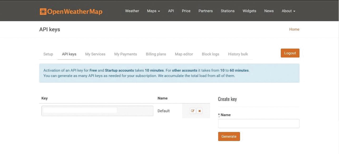
The API tab on OWM’s web site. The API key is hidden for privacy concerns. Never share your API key publicly.
It’s recommended to log in to OWM on the Tinker Board so that you can copy and paste your API key into your code instead of trying to type it, since as you’ll see it’s quite long and a random assortment of letters and numbers.
After you have your key, the next step will be to install the Python library on the Tinker Board. pyowm is installed using pip, so with the terminal navigate to the Home directory using cd ~ and then enter pip install pyowm.
With the library installed, you can start using it to access weather data in Python. The main process for using pyowm is to enter your API key, declare what city you want to collect data for, and then list the types of data that you want. There is an almost endless amount of data available, ranging from the broad to the detailed. The syntax for all of these functions is well documented on the pyowm project’s GitHub.4
The cities are imported by including either the city name with the country code, which is a two-letter abbreviation, or the registry ID, which is a number code assigned to the city and stored in the OWM city registry, which you have access to with the library. These can be accessed in a Python script that we’ll go over now and will also be available on the GitHub repo for this book.
Getting Your City ID
This means that every time owm is listed, it’s referring to your API key. This way, if a feature is not available for your account level, then you won’t be able to pull the data. In our case, this shouldn’t be a problem.
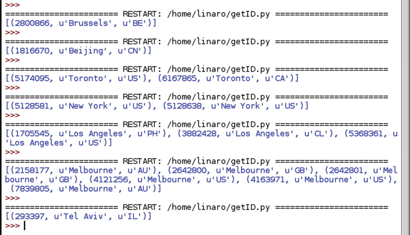
The results of a few example cities displayed in the Python shell that were queried with our script to find city IDs
Python Script for the Weather Display
Now that we have introduced both the EPD’s Python library and the concepts behind the pyowm library, we can begin writing the code for our project. As mentioned earlier, the goal of this project is to use the EPD to display the date, time, and current weather; specifically, the temperature and current forecast. This information can be displayed in a variety of ways since the EPD is essentially a blank canvas.
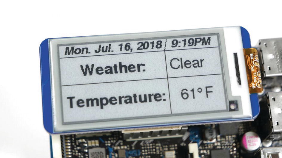
The finished EPD weather display running on the Tinker Board S. You can also use the original Tinker Board as well.
After this, we’ll go into the loop. Because everything on our display will need to be updated in real time, we’ll draw the image and pull the data in the loop. We’ll use while True: to begin the loop and then declare objects and variables for the pyowm library.
First, we’ll declare where the weather data will be collected from, with weather_at_place(), and we’ll also create w = observation.get_weather(), which will be the variable to gather weather data for the pyowm library . Both will be called in the loop so that new data is constantly being gathered; otherwise, we would get the data that was originally pinged when the script was first started. The command w.get_status() is used to get the forecast. This will show things like clear, rain, clouds, snow, and so on. We’re also going to print this to the console for troubleshooting purposes with print w.get_status(). Since w.get_status() outputs a string, it doesn’t need to be modified when used with print.
Note
If you want to use the city ID number instead, you’ll use weather_at_id() rather than weather_at_place()
Next, we’re going to take care of the temperature data. First, we’ll call w.get_temperature('fahrenheit')['temp'], which is the temperature equivalent to get_status(), but with a twist. By putting fahrenheit in the parentheses, the temperature will be read in Fahrenheit, however you can also use Celsius (or even Kelvin), which of course is much more common around the world.
get_temperature() returns a dictionary of temperature data and for our purposes we only need the current temperature, which is cataloged as ['temp'], which is why it’s being called next to get_temperature(). The other issue with ['temp'] is that it has a decimal attached to it, which for the display we’ll want to cut off to show just the base temperature.
To parse this piece of data separately, we’re going to use the math library that we imported earlier to use math.trunc. This completely cuts off the decimal of any number, leaving us with just the whole number; which in this case is the temperature.
The rectangle will be followed by our first text items: the date and time. To do this, we’ll use the time.strftime() function to grab this data in real time. The other aspect of these text entries is the location on the EPD. As discussed, we want these two items to be at the top of the screen and also to be in line with each other. The easiest way to think of this is to see the X axis parameter as asking “how many pixels away from the left side of the screen do you want it to be?” and the Y axis parameter as “how many pixels down from the top of the screen do you want it to be?” This will take some experimentation, since it will all be affected by the font, font size, and length of the string.
For time.strftime('%a. %b. %d, %Y'), the % followed by letters all express different date parameters. In this example, %a will give us the abbreviation for the day of the week, %b will display the abbreviation for the month, %d will give us the number date and %Y will give us the year with the century number. Capitalization does count with this syntax, and you can find more information on all the items available in the time library’s documentation.5
Just as with the date, time.strftime() is used again for the clock, but with different parameters. Here %l is used for the hour, followed by : and then %M is used for the minutes, and %p gives us either AM or PM. Just as with the date, there are more parameters available that are applicable to time-keeping.
For the coordinates, notice that the Y coordinate is the same for both the date and time. This allows them to be lined up with each other.
For the lines, there are two sets of X and Y coordinates. To make it easier to visualize, think of it as finding two points on the display and then drawing the line between them. The first line we draw is going all the way across horizontally below the date and time. The second line is a bit different because it isn’t straight, it’s slanted; resulting in different X values for each coordinate. This is to match the fact that the font we’ve chosen is italicized. The value 25 is used as the second Y coordinate so that it lines up with the horizontal line.
You’ll notice that the Y coordinate is the same for both entries, just as with our date and time data, so that they’ll be lined up. There’s also some space allowed below the previously drawn horizontal line. By calling w.get_status() as the string, we make sure the forecast data output will be constantly updated.
Much like the way we used w.get_status() for the current forecast, we’re doing a similar thing for temperature, where we’re using the temp variable that we wrote earlier to hold the get_temperature() function , which has been broken down to just show the ['temp'] category without the decimal point as a string.
Additionally, this line holds the degree sign and "F" for Fahrenheit. The degree sign is obviously not freely available on a standard keyboard, so instead we’re using Unicode to insert it using chr(176), which is the Unicode character number for the degree sign. The °F is placed next to the temperature data, so that it will always be directly to the right of the temperature, whether it is a single-digit or triple-digit (yikes!) number. Both lines are placed at the same Y coordinate.
The horizontal line crosses directly between the temperature and forecast sections, and the vertical line begins at the same coordinate (25y) as the first horizontal line so that it looks like they’re crossing. This vertical line is straight, unlike the first vertical line, which was diagonal, and crosses the second horizontal line. These lines complete our image so that we can move on to writing it to the memory banks of the EPD hat.
The Technical Parts of the Script
Although the commands are fairly straightforward for displaying to the EPD, getting the placement and sizing just right can take a lot of experimentation and as a result time. However, you truly have a blank canvas to fully customize your project and have it do exactly what you want. There’s just one more step to take this project to the next level…
Autorun Setup
Now that our code is written and working, we’re going to configure it to run automatically when the Tinker Board boots up. This way, you can run this project without having to attach a keyboard, mouse, or display. It can be a standalone Internet-connected device, commonly referred to as headless.
However, the fact that it requires an Internet connection does mean that some special considerations must be made when setting this up. The code will not execute without an active connection, because of the pyowm library for our weather data, so it needs to be configured to execute only after the Tinker Board has booted up and there is also an active network connection present.
To do this, we’ll set up our Python script to be executable, so that it can launch on its own. Then we’ll place the script and its dependencies into a folder found under /etc/network called if-up.d. This folder contains scripts that automatically run once a network connection is established (thus the naming convention “if-up”). The only caveat here is that this folder requires root access. Files cannot simply be dragged and dropped into it. For that reason, we’ll be doing this work through the terminal.
Note
Although everything is being done through the terminal, it’s recommended to have the GUI file directory open to the if-up.d folder to double-check that everything is working properly.
Save your script and then open a terminal, changing directories to your project’s folder, and enter chmod a+x weatherDisplay.py. Nothing will seem to happen in the terminal, but if you click the file in the GUI, you’ll be given the choice to run the script without any other commands. You can also run it via the terminal with sudo ./weatherDisplay.py.
Speaking of our script’s name, we need to remove the .py extension for this method to work properly. We can do this easily in the GUI by right-clicking the file and renaming it. We need to do this because any files that have an extension like that will not run in the if-up.d folder.
root@tinkerboard in the terminal
Note
You may need to place copies of the Python libraries, including pyowm, into the projectFolder depending on how you’ve set up Python and pip directories on your Tinker Board. It will also depend on how future iterations of TinkerOS and the kernel handle this as well.
Basically, you’re using the copy command, cp, and then listing the file location of the folder you wish to copy, followed by a space, and then the file location of the folder where you want to copy your original folder to; also known as the target folder.
Note the space between the last * and . at the end of the line. By entering the file extension of the project folder with that syntax, you ensure that all folders and files are moved up a level, even if their file names begin with a period (.). Omitting the space could cause errors; especially when dealing with code library files that may use unique naming conventions. After executing the command, you should see all the files and folders from the project folder appear directly into the if-up.d folder.
Everything should be ready to go, but first we need to clean things up a bit. The project folder is empty now and is no longer necessary, so we should remove it. We’ll do that using the rm (remove) command. This is a very powerful command; once you execute it, it will immediately remove the targeted file or folder, so always be cautious when using it.
The rm command has different flags for whether you are deleting a single file or an entire folder. The flag for a folder, or directory, is -r. Also, instead of typing out the entire file directory location, you’ll only include the name of the folder you’re removing. So, the command to remove the now empty project folder inside if-up.d is rm -r projectFolder. You should see the folder disappear from the file directory GUI.
Before we reboot to see if our script starts up correctly with a network connection, we should test to make sure the script can run properly from the if-up.d folder. Run the script in the terminal using ./weatherDisplay (no sudo is needed, since we’re still root) to make sure that no errors appear. If you get any missing dependency errors, then you’ll need to copy those library folders, as mentioned previously in the note, over to the if-up.d folder. You can use the same cp process for this that we went over earlier.
If the EPD displays as expected, then it’s time to reboot the Tinker Board using reboot. If all goes as planned, then after TinkerOS boots to the desktop with a successful network connection you should see the EPD begin the script by doing the full update and then updating the date, time, and weather in real time.
Finishing Touches
With all the coding and Linux work done, you have a fully functional Internet-connected information display. Because it is headless, you can place it anywhere with a connection to power, and have it run. There are some aesthetic things you can do, though, to bring it to the next level.
Instead of simply leaving the Tinker Board with the EPD display exposed to the elements, you can put it in a housing of some sort. As we discussed in the first chapter, there are a variety of cases available that will fit the Tinker Board’s form factor. Many of these cases have openings to allow access to the GPIO pins and as a result, the Tinker Board could be protected from environmental and physical hazards while having the EPD display remain attached and unaffected by the housing.
There are also fully DIY options out there with the only limitation being your imagination. There’s always the option of 3D printing or milling a custom case. Another popular option for EPD projects is to utilize a picture frame, or similarly functional household item, to allow the display to blend in with its surroundings in a home.
Of course, you aren’t just limited to showing the data parameters that we coded for in this project. These displays can basically show any information that you want. There are many calendar, news, and social media APIs available for Python that you can utilize in your code to fully customize the kind of EPD project that you want. You can also animate these displays further with the PIL library and integrate them with larger projects.
This chapter has shown how you can integrate programming with the Tinker Board to create fully customized projects and given you the tools to go further with your own ideas; which has truly been the goal of this entire book. We have one more project in front of us, and it is a classic: a robot!