A vector is defined as an object with both magnitude and direction. This definition, however, is a bit complicated. For our purpose, a vector is simply a 1-dimensional array representing a series of numbers. Put another way, a vector is a list of numbers.

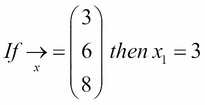
It is generally represented using an arrow or bold font, shown as follows:

Vectors are broken into components, which are individual members of the vector. We use index notations to denote the element that we are referring to, illustrated as follows:

In Python, we can represent arrays in many ways. We could simply use a Python list to represent the preceding array:

x = [3, 6, 8] 

However, it is better to use the numpy array type to represent arrays, as shown, because it gives us much more utility when performing vector operations:

import numpy as np 
x = np.array([3, 6, 8]) 

Regardless of the Python representation, vectors give us a simple way of storing multiple dimensions of a single data point/observation.

If we measure the average satisfaction rating (0-100) of employees in three departments of a company as being 57 for HR, 89 for engineering, and 94 for management. We can represent this as a vector with the following formula:

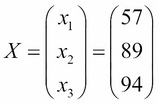
This vector holds three different bits of information about our data. This is the perfect use of a vector in data science.

You can also think of a vector as being the theoretical generalization of the pandas Series object. So, naturally, we need something to represent the DataFrame.

We can extend our notion of an array to move beyond a single dimension and represent data in multiple dimensions.

A matrix is a two-dimensional representation of arrays of numbers. Matrices (plural) have two main characteristics that we need to be aware of. The dimension of a matrix, denoted by n x m (n by m), tells us that the matrix has n rows and m columns. Matrices are generally denoted by a capital, bold-faced letter, such as X. Consider the following example:

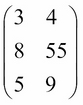
This is a 3 x 2 (3 by 2) matrix because it has three rows and two columns.

The matrix is our generalization of the pandas DataFrame. It is arguably one of the most important mathematical objects in our toolkit. It is used to hold organized information, in our case, data.

Revisiting our previous example, let's say we have three offices in different locations, each with the same three departments: HR, engineering, and management. We could make three different vectors, each holding a different office's satisfaction scores, as shown:

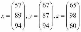
However, this is not only cumbersome, but also unscalable. What if you have 100 different offices? Then you would need to have 100 different one-dimensional arrays to hold this information.

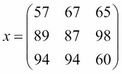
This is where a matrix alleviates this problem. Let's make a matrix where each row represents a different department and each column represents a different office, as shown:

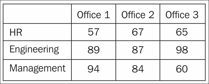
This is much more natural. Now, let's strip away the labels, and we are left with a matrix!

In this section, we will go over some symbols associated with basic arithmetic that appear in most, if not all, data science tutorials and books.

Summation

The uppercase sigma ∑ symbol is a universal symbol for addition. Whatever is to the right of the sigma symbol is usually something iterable, meaning that we can go over it one by one (for example, a vector).

For example, let's create the representation of a vector:

X = [1, 2, 3, 4, 5] 

To find the sum of the content, we can use the following formula:

In Python, we can use the following formula:

sum(x) # == 15 

For example, the formula for calculating the mean of a series of numbers is quite common. If we have a vector (x) of length n, the mean of the vector can be calculated as follows:

This means that we will add up each element of x, denoted by xi, and then multiply the sum by 1/n, otherwise known as dividing by n, (the length of the vector).

Dot product

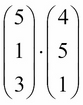
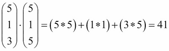
The dot product is an operator like addition and multiplication. It is used to combine two vectors, as shown:

So, what does this mean? Let's say we have a vector that represents a customer's sentiments toward three genres of movies: comedy, romance, and action.

Note

When using a dot product, note that an answer is a single number, known as a scalar.

On a scale of 1-5, a customer loves comedies, hates romantic movies, and is alright with action movies. We might represent this as follows:

Here, 5 denotes their love for comedies, 1 their hatred of romantic movies, and 3 the customer's indifference toward action movies.

Now, let's assume that we have two new movies, one of which is a romantic comedy and the other is a funny action movie. The movies would have their own vector of qualities, as shown:

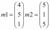
Here, m1 is our romantic comedy and m2 is our funny action movie.

In order to make a recommendation, we will apply the dot product between the customer's preferences for each movie. The higher value will win and, therefore, will be recommended to the user.

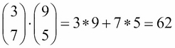
Let's compute the recommendation score for each movie. For movie 1, we want to compute the following:

We can think of this problem like as follows:

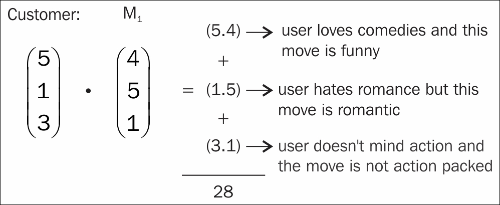
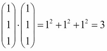
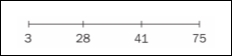
The answer we obtain is 28, but what does this number mean? On what scale is it? Well, the best score anyone can ever get is when all values are 5, making the outcome as follows:

The lowest possible score is when all values are 1, as shown:

So, we must think about 28 on a scale from 3 to 75. To do this, imagine a number line from 3 to 75 and where 28 would be on it. This is illustrated as follows:

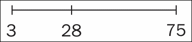
Not that far. Let's try for movie 2:

This is higher than 28! Putting this number on the same timeline as before, we can also visually observe that it is a much better score, as shown:

So, between movie 1 and movie 2, we would definitely recommend movie 2 to our user. This is, in essence, how most movie prediction engines work. They build a customer profile, which is represented as a vector. They then take a vector representation of each movie they have to offer, combine them with the customer profile (perhaps with a dot product), and make recommendations from there. Of course, most companies must do this on a much larger scale, which is where a particular field of mathematics, called linear algebra, can be very useful; we will look at it later in the chapter.

No doubt you have encountered dozens, if not hundreds, of graphs in your life so far. I'd like to mostly talk about conventions with regard to graphs and notations.

The following is a basic Cartesian graph (x and y coordinates). The x and y notations are very standard but sometimes do not entirely explain the big picture. We sometimes refer to the x variable as being the independent variable and the y as the dependent variable. This is because when we write functions, we tend to speak about them as being y is a function of x, meaning that the value of y is dependent on the value of x. This is what a graph is trying to show.

Suppose we have two points on a graph, as shown:

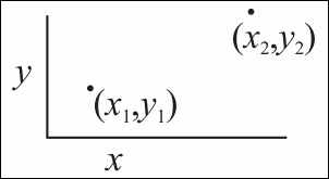
We refer to the points as (x1, y1) and (x2, y2).

The slope between these two points is defined as follows:

You have probably seen this formula before, but it is worth mentioning, if only for its significance. The slope defines the rate of change between the two points. Rates of change can be very important in data science, specifically in areas involving differential equations and calculus.

Rates of change are a way of representing how variables move together and to what degree. Imagine we are modeling the temperature of your coffee in relation to the time that it has been sitting outside. Perhaps we have a rate of change as follows:

This rate of change is telling us that for every single minute, our coffee's temperature is dropping by two degrees Fahrenheit.

Later on in this book, we will look at a machine learning algorithm called linear regression. In linear regression, we are concerned with the rates of change between variables, as they allow us to exploit this relationship for predictive purposes.

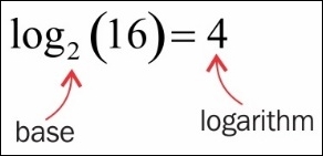
An exponent tells you how many times you have to multiply a number by itself, as illustrated:

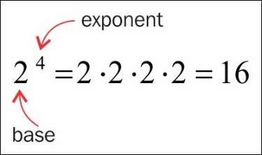
A logarithm is the number that answers the question "what exponent gets me from the base to this other number?" This can be denoted as follows:

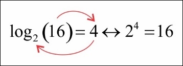
If these two concepts seem similar, then you are correct! Exponents and logarithms are heavily related. In fact, the words exponent and logarithm actually mean the same thing! A logarithm is an exponent. The preceding two equations are actually two versions of the same thing. The basic idea is that 2 times 2 times 2 times 2 is 16.

The following is a depiction of how we can use both versions to say the same thing. Note how I use arrows to move from the log formula to the exponent formula:

Consider the following examples:

Note something interesting. Let's rewrite the first equation:

We then replace 81 with the equivalent statement, , as follows:

Something interesting to note: the 3s seem to cancel out. This is actually very important when dealing with numbers more difficult to work with than 3s and 4s.

Exponents and logarithms are most important when dealing with growth. More often than not, if a quantity is growing (or declining in growth), an exponent/logarithm can help model this behavior.

For example, the number e is around 2.718 and has many practical applications. A very common application is interest calculation for saving. Suppose you have $5,000 deposited in a bank with continuously compounded interest at the rate of 3%, then we can use the following formula to model the growth of your deposit:

In this formula:

We are curious; when will our investment double? How long would I have to have my money in this investment to achieve 100% growth? We can write this in mathematical form, as follows:

(divided by 5000 on both sides)

At this point, we have a variable in the exponent that we want to solve. When this happens, we can use the logarithm notation to figure it out:

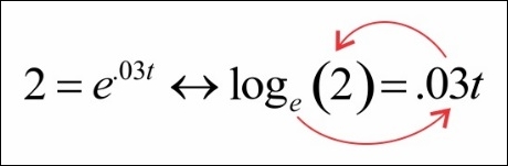
This leaves us with .

When we take the logarithm of a number with a base of e, it is called a natural logarithm. We rewrite the logarithm as follows:

Using a calculator (or Python), we find that :

This means that it would take 2.31 years to double our money.

Set theory involves mathematical operations at the set level. It is sometimes thought of as a basic fundamental group of theorems that governs the rest of mathematics. For our purpose, we'll use set theory to manipulate groups of elements.

A set is a collection of distinct objects.

That's it! A set can be thought of as a list in Python, but with no repeat objects. In fact, there is even a set of objects in Python:

s = set() 
 
s = set([1, 2, 2, 3, 2, 1, 2, 2, 3, 2]) 
# will remove duplicates from a list 
 
s == {1, 2, 3} 

Remember that a dictionary in Python is a set of key-value pairs, for example:

dict = {"dog": "human's best friend", "cat": "destroyer of world"} 
dict["dog"]# == "human's best friend" 
len(dict["cat"]) # == 18 
 
# but if we try to create a pair with the same key as an existing key 
dict["dog"] = "Arf" 
 
dict 
{"dog": "Arf", "cat": "destroyer of world"} 
# It will override the previous value 
# dictionaries cannot have two values for one key.

They share this notation because they share a quality in that sets cannot have duplicate elements, just as dictionaries cannot have duplicate keys.

The magnitude of a set is the number of elements in the set and is represented as follows:

s  # == {1,2,3} 
len(s) == 3 # magnitude of s 

If we wish to denote that an element is within a set, we use the epsilon notation, as shown:

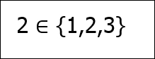
This means that the 2 element exists in the set of 1, 2, and 3. If one set is entirely inside another set, we say that it is a subset of its larger counterpart:

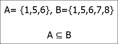
So, A is a subset of B and B is called the superset of A. If A is a subset of B but A does not equal B (meaning that there is at least one element in B that is not in A), then A is called a proper subset of B.

Consider the following examples:

In data science, we use sets (and lists) to represent a list of objects and, often, to generalize the behavior of consumers. It is common to reduce a customer to a set of characteristics.

Imagine we are a marketing firm trying to predict where a person wants to shop for clothes. We are given a set of clothing brands the user has previously visited, and our goal is to predict a new store that they would also enjoy. Suppose a specific user has previously shopped at the following stores:

user1 = {"Target","Banana Republic","Old Navy"}  
# note that we use {} notation to create a set 
# compare that to using [] to make a list 

So, user1 has previously shopped at Target, Banana Republic, and Old Navy. Let's also look at a different user, called user2, as shown:

user2 = {"Banana Republic","Gap","Kohl's"}

Suppose we are wondering how similar these users are. With the limited information we have, one way to define similarity is to see how many stores there are that they both shop at. This is called an intersection:

The intersection of two sets is a set whose elements appear in both sets. It is denoted using the ∩ symbol, as shown:

The intersection of the two users is just one store. So, right away, that doesn't seem great. However, each user only has three elements in their set, so having 1/3 does not seem as bad. Suppose we are curious about how many stores are represented between the two of them; this is called a union.

The union of two sets is a set whose elements appear in either set. It is denoted using the symbol ∪, as shown:

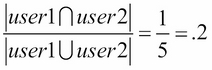
When looking at the similarities between user1 and user2, we should use a combination of the union and the intersection of their sets. user1 and user2 have one element in common out of a total of five distinct elements between them. So, we can define the similarity between the two users as follows:

In fact, this has a name in set theory. It is called the Jaccard measure. In general, for the A and B sets, the Jaccard measure (Jaccard similarity) between the two sets is defined as follows:

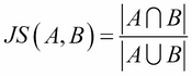
It can also be defined as the magnitude of the intersection of the two sets divided by the magnitude of the union of the two sets.

This gives us a way to quantify similarities between elements represented with sets.

Intuitively, the Jaccard measure is a number between 0 and 1, such that when the number is closer to 0, people are more dissimilar and when the measure is closer to 1, people are considered similar to each other.

If we think about the definition, then it actually makes sense. Take a look at the measure once more:

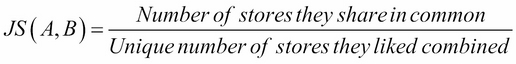
Here, the numerator represents the number of stores that the users have in common (in the sense that they like shopping there), while the denominator represents the unique number of stores that they like put together.

We can represent this in Python using some simple code, as shown:

user1 = {"Target","Banana Republic","Old Navy"}  
user2 = {"Banana Republic","Gap","Kohl's"} 
 
def jaccard(user1, user2): 
  stores_in_common = len(user1 & user2) 
  stores_all_together = len(user1 | user2) 
  return stores / float(stores_all_together) 
 
# I cast stores_all_together as a float to return a decimal answer instead of python's default integer division 
 
# so 
jaccard(user1, user2) == # 0.2 or 1/5 

Set theory becomes highly prevalent when we enter the world of probability and also when dealing with high-dimensional data. We will use sets to represent real-world events taking place, and probability becomes set theory with vocabulary on top of it.