The Silhouette Coefficient is a common metric for evaluating clustering performance in situations when the true cluster assignments are not known.

A Silhouette Coefficient is calculated for each observation as follows:

Let's look a little closer at the specific features of this formula:

It ranges from -1 (worst) to 1 (best). A global score is calculated by taking the mean score for all observations. In general, a Silhouette Coefficient of 1 is preferred, while a score of -1 is not preferable:

# calculate Silhouette Coefficient for K=3 
from sklearn import metrics 
metrics.silhouette_score(X, km.labels_)

The output is as follows:

0.67317750464557957

Let's try calculating the coefficient for multiple values of K to find the best value:

# center and scale the datafrom sklearn.preprocessing import StandardScalerscaler = StandardScaler()X_scaled = scaler.fit_transform(X)# calculate SC for K=2 through K=19 
k_range = range(2, 20) 
scores = [] 
for k in k_range: 
    km = KMeans(n_clusters=k, random_state=1) 
    km.fit(X_scaled) 
    scores.append(metrics.silhouette_score(X, km.labels_)) 
 
# plot the results 
plt.plot(k_range, scores) 
plt.xlabel('Number of clusters') 
plt.ylabel('Silhouette Coefficient') 
plt.grid(True)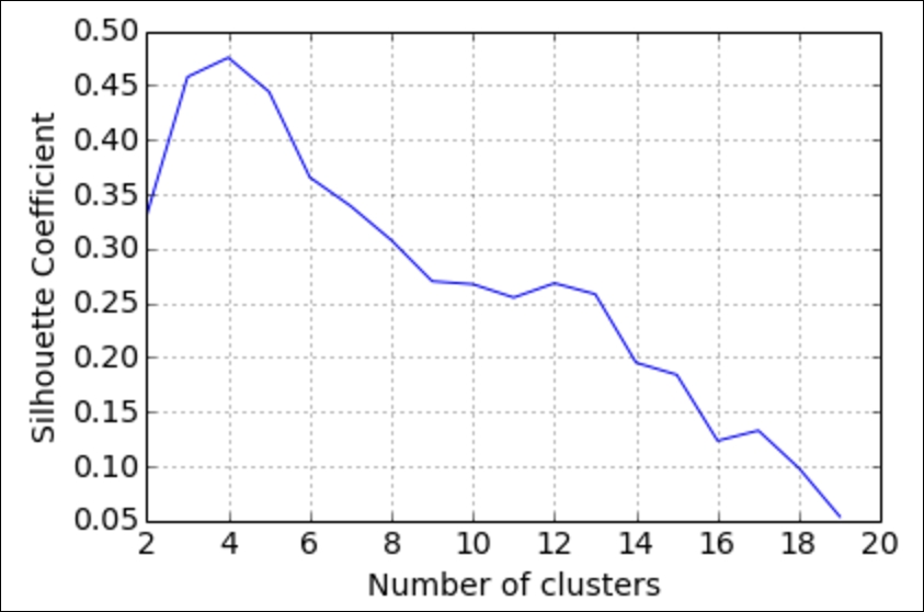 

So, it looks like our optimal number of beer clusters is 4! This means that our k-means algorithm has determined that there seem to be four distinct types of beer.

k-means is a popular algorithm because of its computational efficiency and simple and intuitive nature. k-means, however, highly scale dependent and is not suitable for data with widely varying shapes and densities. There are ways to combat this issue by scaling data using scikit-learn's standard scalar:

# center and scale the data 
from sklearn.preprocessing import StandardScaler 
scaler = StandardScaler() 
X_scaled = scaler.fit_transform(X) 
 
# K-means with 3 clusters on scaled data 
km = KMeans(n_clusters=3, random_state=1) 
km.fit(X_scaled) 

Easy!

Now let's take a look at the third reason to use unsupervised methods that falls under the third option in our reasons to use unsupervised methods: feature extraction.

Sometimes we have an overwhelming number of columns and likely not enough rows to handle the great quantity of columns.

A great example of this is when we were looking at the send cash now example in our Nave Bayes example. We had literally 0 instances of texts with that exact phrase, so instead, we turned to a naïve assumption that allowed us to extrapolate a probability for both of our categories.

The reason we had this problem in the first place is because of something called the curse of dimensionality. The curse of dimensionality basically says that as we introduce and consider new feature columns, we need almost exponentially more rows (data points) in order to fill in the empty spaces that we create.

Consider an example where we attempt to use a learning model that utilizes the distance between points on a corpus of text that has 4,086 pieces of text and that the whole thing has been Countvectorized. Let's assume that these texts between them have 18,884 words:

X.shape

The output is as follows:

(20, 4)

Now, let's do an experiment. I will first consider a single word as the only dimension of our text. Then, I will count how many of pieces of text are within 1 unit of each other. For example, if two sentences both contain that word, they would be 0 units away and, similarly, if neither of them contain the word, they would be 0 units away from one another:

d = 1 
# Let's look for points within 1 unit of one another 
 
X_first_word = X.iloc[:,:1] 
# Only looking at the first column, but ALL of the rows 
 
from sklearn.neighbors import NearestNeighbors 
# this module will calculate for us distances between each point 
 
neigh = NearestNeighbors(n_neighbors=4086) 
neigh.fit(X_first_word) 
# tell the module to calculate each distance between each point 

A = neigh.kneighbors_graph(X_first_word, mode='distance').todense() 
# This matrix holds all distances (over 16 million of them) 
 
num_points_within_d = (A < d).sum() 
# Count the number of pairs of points within 1 unit of distance 
 
num_points_within_d 
16258504
So, 16.2 million pairs of texts are within a single unit of distance. Now, let's try again with the first two words:
X_first_two_words = X.iloc[:,:2] 
neigh = NearestNeighbors(n_neighbors=4086) 
neigh.fit(X_first_two_words) 
A = neigh.kneighbors_graph(X_first_two_words, mode='distance').todense() 
num_points_within_d = (A < d).sum() 
 
num_points_within_d 
16161970 

Great! By adding this new column, we lost about 100,000 pairs of points that were within a single unit of distance. This is because we are adding space in between them for every dimension that we add. Let's take this test a step further and calculate this number for the first 100 words and then plot the results:

d = 1 
# Scan for points within one unit 
 
num_columns = range(1, 100) 
# Looking at the first 100 columns 
points = [] 
# We will be collecting the number of points within 1 unit for a graph 
 
neigh = NearestNeighbors(n_neighbors=X.shape[0]) 
for subset in num_columns: 
    X_subset = X.iloc[:,:subset] 
  # look at the first column, then first two columns, then first three columns, etc 
    neigh.fit(X_subset) 
    A = neigh.kneighbors_graph(X_subset, mode='distance').todense() 
    num_points_within_d = (A < d).sum() 
# calculate the number of points within 1 unit 
    points.append(num_points_within_d) 

Now, let's plot the number of points within 1 unit versus the number of dimensions we looked at:

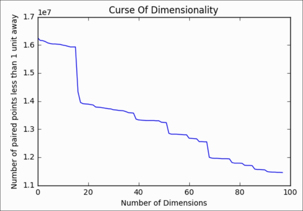
We can see clearly that the number of points within a single unit of one another goes down dramatically as we introduce more and more columns. And this is only the first 100 columns! Let's see how many points are within a single unit by the time we consider all 18,000+ words:

neigh = NearestNeighbors(n_neighbors=4086) 
neigh.fit(X) 
A = neigh.kneighbors_graph(X, mode='distance').todense() 
num_points_within_d = (A < d).sum() 
 
 
num_points_within_d 
4090 

By the end, only 4,000 sentences are within a unit of one another. All of this space that we add in by considering new columns makes it harder for the finite amount of points we have to stay happily within range of each other. We would have to add in more points in order to fill in this gap. And that, my friends, is why we should consider using dimension reduction.

The curse of dimensionality is solved by either adding more data points (which is not always possible) or implementing dimension reduction. Dimension reduction is simply the act of reducing the number of columns in our dataset and not the number of rows. There are two ways of implementing dimension reduction:

We are familiar with feature selection as the process of saying the "Embarked_Q" is not helping my decision tree; let's get rid of it and see how it performs. It is literally when we (or the machine) make the decision to ignore certain columns.

Feature extraction is a bit trickier…

In feature extraction, we are using usually fairly complicated mathematical formulas in order to obtain new super columns that are usually better than any single original column.

Our primary model for doing so is called Principal Component Analysis (PCA). PCA will extract a set number of super columns in order to represent our original data with much fewer columns. Let's take a concrete example. Previously, I mentioned some text with 4,086 rows and over 18,000 columns. That dataset is actually a set of Yelp online reviews:

url = '../data/yelp.csv' 
yelp = pd.read_csv(url, encoding='unicode-escape') 
 
# create a new DataFrame that only contains the 5-star and 1-star reviews 
yelp_best_worst = yelp[(yelp.stars==5) | (yelp.stars==1)] 
 
# define X and y 
X = yelp_best_worst.text 
y = yelp_best_worst.stars == 5 

Our goal is to predict whether or not a person gave a 5- or 1-star review based on the words they used in the review. Let's set a base line with logistic regression and see how well we can predict this binary category:

from sklearn.linear_model import LogisticRegression 
lr = LogisticRegression() 
 
X_train, X_test, y_train, y_test = train_test_split(X, y, random_state=100) 
# Make our training and testing sets 
 
vect = CountVectorizer(stop_words='english') 
# Count the number of words but remove stop words like a, an, the, you, etc 
 
X_train_dtm = vect.fit_transform(X_train) 
X_test_dtm = vect.transform(X_test) 
# transform our text into document term matrices 
 
lr.fit(X_train_dtm, y_train) 
# fit to our training set 
 
lr.score(X_test_dtm, y_test) 
# score on our testing set

The output is as follows:

0.91193737

So, by utilizing all of the words in our corpus, our model seems to have over a 91% accuracy. Not bad!

Let's try only using the top 100 used words:

vect = CountVectorizer(stop_words='english', max_features=100) 
# Only use the 100 most used words 
X_train_dtm = vect.fit_transform(X_train) 
X_test_dtm = vect.transform(X_test) 
print( X_test_dtm.shape) # (1022, 100) 

lr.fit(X_train_dtm, y_train) 

lr.score(X_test_dtm, y_test) 

The output is as follows:

0.8816

Note how our training and testing matrices have 100 columns. This is because I told our vectorizer to only look at the top 100 words. See also that our performance took a hit and is now down to 88% accuracy. This makes sense because we are ignoring over 4,700 words in our corpus.

Now, let's take a different approach. Let's import a PCA module and tell it to make us 100 new super columns and see how that performs:

from sklearn import decomposition 
# We will be creating 100 super columns 

vect = CountVectorizer(stop_words='english') 
# Don't ignore any words 
pca = decomposition.PCA(n_components=100) 
# instantate a pca object X_train_dtm = vect.fit_transform(X_train).todense() 
# A dense matrix is required to pass into PCA, does not affect the overall message 

X_train_dtm = pca.fit_transform(X_train_dtm) 

X_test_dtm = vect.transform(X_test).todense() 
X_test_dtm = pca.transform(X_test_dtm) 
print( X_test_dtm.shape) # (1022, 100) 

lr.fit(X_train_dtm, y_train) 

lr.score(X_test_dtm, y_test) 

The output is as follows:

.89628

Not only do our matrices still have 100 columns, but these columns are no longer words in our corpus. They are complex transformations of columns and are 100 new columns. Also note that using 100 of these new columns gives us a better predictive performance than using the 100 top words!

Feature extraction is a great way to use mathematical formulas to extract brand new columns that generally perform better than just selecting the best ones beforehand.

But how do we visualize these new super columns? Well, I can think of no better way than to look at an example using image analysis. Specifically, let's make facial recognition software. OK? OK. Let's begin by importing some faces given to us by scikit-learn:

from sklearn.datasets import fetch_lfw_people
 
lfw_people = fetch_lfw_people(min_faces_per_person=70, resize=0.4)
 
# introspect the images arrays to find the shapes (for plotting)
n_samples, h, w = lfw_people.images.shape
# for machine learning we use the 2 data directly (as relative pixel # positions info is ignored by this model)
X = lfw_people.data
y = lfw_people.target
n_features = X.shape[1]

X.shape (1288, 1850)

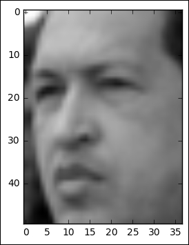
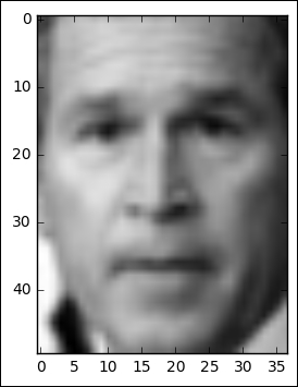
We have gathered 1,288 images of people's faces, and each one has 1,850 features (pixels) that identify that person. Here's an example:

plt.imshow(X[0].reshape((h, w)), cmap=plt.cm.gray) lfw_people.target_names[y[0]] 'Hugo Chavez'

plt.imshow(X[100].reshape((h, w)), cmap=plt.cm.gray) lfw_people.target_names[y[100]] 'George W Bush'

Great. To get a glimpse at the type of dataset we are looking at, let's look at a few overall metrics:

# the label to predict is the id of the person 
target_names = lfw_people.target_names 
n_classes = target_names.shape[0] 
print("Total dataset size:") 
print("n_samples: %d" % n_samples) 
print("n_features: %d" % n_features) 
print("n_classes: %d" % n_classes) 
Total dataset size: 
n_samples: 1288 
n_features: 1850

n_classes: 7

So, we have 1,288 images, 1,850 features, and 7 classes (people) to choose from. Our goal is to make a classifier that will assign the person's face a name based on the 1,850 pixels given to us.

Let's take a base line and see how logistic regression performs on our data without doing anything:

from sklearn.linear_model import LogisticRegression
from sklearn.metrics import accuracy_score
from time import time # for timing our work
X_train, X_test, y_train, y_test = train_test_split(
X, y, test_size=0.25, random_state=1)
# get our training and test set
t0 = time() # get the time now
logreg = LogisticRegression()
logreg.fit(X_train, y_train)
# Predicting people's names on the test set
y_pred = logreg.predict(X_test)
print( accuracy_score(y_pred, y_test), "Accuracy")

print( (time() - t0), "seconds" )

The output is as follows:

0.810559006211 Accuracy
6.31762504578 seconds

So, within 6.3 seconds, we were able to get an 81% on our test set. Not too bad.

Now let's try this with our super faces:

# split into a training and testing set 
from sklearn.cross_validation import train_test_split 

# Compute a PCA (eigenfaces) on the face dataset (treated as unlabeled # dataset): unsupervised feature extraction / dimensionality reduction n_components = 75 

print("Extracting the top %d eigenfaces from %d faces"
% (n_components, X_train.shape[0])) 
pca = decomposition.PCA(n_components=n_components, whiten=True).fit(X_train) 
# This whiten parameter speeds up the computation of our extracted columns 
# Projecting the input data on the eigenfaces orthonormal basis 
X_train_pca = pca.transform(X_train)
 
X_test_pca = pca.transform(X_test)

The preceding code is collecting 75 extracted columns from our 1,850 unprocessed columns. These are our super faces. Now, let's plug in our newly extracted columns into our logistic regression and compare:

t0 = time()
# Predicting people's names on the test set WITH PCA
logreg.fit(X_train_pca, y_train)
y_pred = logreg.predict(X_test_pca)
print accuracy_score(y_pred, y_test), "Accuracy"
print (time() - t0), "seconds"
0.82298136646 Accuracy

0.194181919098 seconds

Wow! Not only was this entire calculation about 30 times faster than the unprocessed images, but the predictive performance also got better! This shows us that PCA and feature extraction, in general, can help us all around when performing machine learning on complex datasets with many columns. By searching for these patterns in the dataset and extracting new feature columns, we can speed up and enhance our learning algorithms.

Let's look at one more interesting thing. I mentioned before that one of the purposes of this example was to examine and visualize our eigenfaces, as they are called: our super columns. I will not disappoint. Let's write some code that will show us our super columns as they would look to us humans:

def plot_gallery(images, titles, n_row=3, n_col=4):
"""Helper function to plot a gallery of portraits"""
plt.figure(figsize=(1.8 * n_col, 2.4 * n_row))
plt.subplots_adjust(bottom=0, left=.01, right=.99, top=.90, hspace=.35)
for i in range(n_row * n_col):
plt.subplot(n_row, n_col, i + 1)
plt.imshow(images[i], cmap=plt.cm.gray)
plt.title(titles[i], size=12) 
# plot the gallery of the most significative eigenfaces
eigenfaces = pca.components_.reshape((n_components, h, w))
eigenface_titles = ["eigenface %d" % i for i in range(eigenfaces.shape[0])]
plot_gallery(eigenfaces, eigenface_titles)

plt.show()

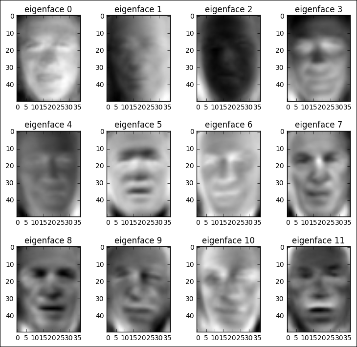
Wow. A haunting and yet beautiful representation of what the data believes to be the most importance features of a face. As we move from the top-left (first super column) to the bottom, it is actually somewhat easy to see what the image is trying to tell us. The first super column looks like a very general face structure with eyes and nose and a mouth. It is almost saying "I represent the basic qualities of a face that all faces must have." Our second super column directly to its right seems to be telling us about shadows in the image. The next one might be telling us that skin tone plays a role in detecting who this is, which might be why the third face is much darker than the first two.

Using feature extraction unsupervised learning methods such as PCA can give us a very deep look into our data and reveal to us what the data believes to be the most important features, not just what we believe them to be. Feature extraction is a great preprocessing tool that can speed up our future learning methods, make them more powerful, and give us more insight into how the data believes it should be viewed. To sum up this section, we will list the pros and cons.

Here are the pros of using feature extraction:

And here are the cons of using feature extraction:

We lose some of the interpretability of our features as they are new mathematically-derived columns, not our old ones

We can lose predictive performance because we are losing information as we extract fewer columns