Neural networks are made up of interconnected nodes (perceptrons) that each take in input (quantitative value), and output other quantitative values. Signals travel through the network and eventually end up at a prediction node:

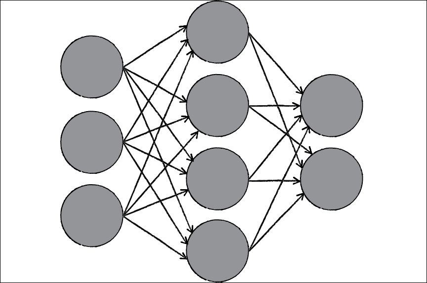
Visualization of neural network interconnected nodes

Another huge advantage of neural networks is that they can be used for supervised learning, unsupervised learning, and reinforcement learning problems. The ability to be so flexible, predict many functional shapes, and adapt to their surroundings make neural networks highly preferable in select fields, as follows:

The simplest form of a neural network is a single perceptron. A perceptron, visualized as follows, takes in some input and outputs a signal:

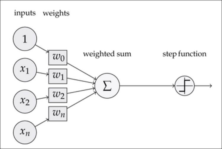
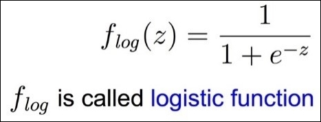
This signal is obtained by combining the input with several weights and then is put through some activation function. In cases of simple binary outputs, we generally use the logistic function, as shown:

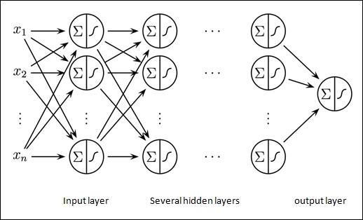
To create a neural network, we need to connect multiple perceptrons to each other in a network fashion, as illustrated in the following graph.

A multilayer perceptron (MLP) is a finite acyclic graph. The nodes are neurons with logistic activation:

As we train the model, we update the weights (which are random at first) of the model in order to get the best predictions possible. If an observation goes through the model and is outputted as false when it should have been true, the logistic functions in the single perceptrons are changed slightly. This is called back-propagation. Neural networks are usually trained in batches, which means that the network is given several training data points at once several times, and each time, the back-propagation algorithm will trigger an internal weight change in the network.

It isn't hard to see that we can grow the network very deep and have many hidden layers, which are associated with the complexity of the neural network. When we grow our neural networks very deep, we are dipping our toes into the idea of deep learning. The main advantage of deep neural networks (networks with many layers) is that they can approximate almost any shape function and they can (theoretically) learn optimal combinations of features for us and use these combinations to obtain the best predictive power.

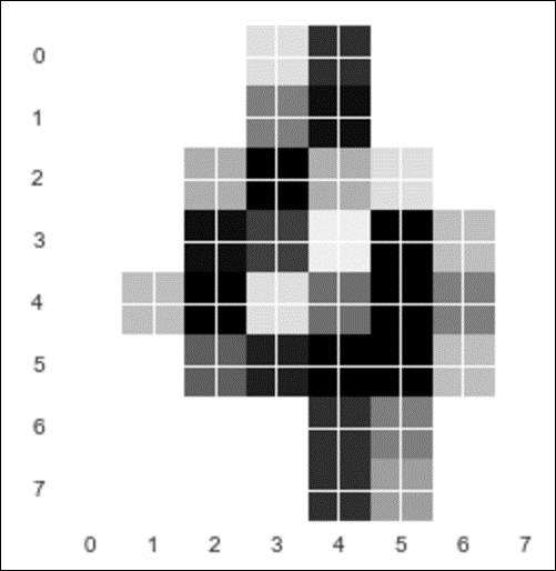
Let's see this in action. I will be using a module called PyBrain to make my neural networks. However, first let's take a look at a new dataset, which is a dataset of handwritten digits. We will first try to recognize digits using a random forest, as shown:

from sklearn.cross_validation import cross_val_score 
from sklearn import datasets 
import matplotlib.pyplot as plt 
from sklearn.ensemble import RandomForestClassifier 
%matplotlib inline 
 
digits = datasets.load_digits() 
 
plt.imshow(digits.images[100], cmap=plt.cm.gray_r, interpolation='nearest') 
# a 4 digit 

X, y = digits.data, digits.target 
 
# 64 pixels per image 
X[0].shape 
 
# Try Random Forest 
rfclf = RandomForestClassifier(n_estimators=100, random_state=1) 
cross_val_score(rfclf, X, y, cv=5, scoring='accuracy').mean() 
0.9382782 

Pretty good! An accuracy of 94% is nothing to laugh at, but can we do even better?

from pybrain.datasets            import ClassificationDataSet 
from pybrain.utilities           import percentError 
from pybrain.tools.shortcuts     import buildNetwork 
from pybrain.supervised.trainers import BackpropTrainer 
from pybrain.structure.modules   import SoftmaxLayer 
from numpy import ravel 
 
 
 
# pybrain has its own data sample class that we must add 
# our training and test set to 
ds = ClassificationDataSet(64, 1 , nb_classes=10) 
for k in xrange(len(X)):  
    ds.addSample(ravel(X[k]),y[k]) 
     
# their equivalent of train test split 
test_data, training_data = ds.splitWithProportion( 0.25 ) 
 
 
 
 
# pybrain's version of dummy variables 
 
test_data._convertToOneOfMany( ) 
training_data._convertToOneOfMany( ) 
 
 
print test_data.indim # number of pixels going in 
# 64 
print test_data.outdim # number of possible options (10 digits) 
# 10 
 
 
 
# instantiate the model with 64 hidden layers (standard params) 
fnn = buildNetwork( training_data.indim, 64, training_data.outdim, outclass=SoftmaxLayer ) 
trainer = BackpropTrainer( fnn, dataset=training_data, momentum=0.1, learningrate=0.01 , verbose=True, weightdecay=0.01)  
 
# change the number of epochs to try to get better results! 
trainer.trainEpochs (10) # 10 batches 
print 'Percent Error on Test dataset: ' ,  
        percentError( trainer.testOnClassData ( 
           dataset=test_data ) 
           , test_data['class'] ) 

The model will output a final error on a test set:

Percent Error on Test dataset: 4.67706013363 
accuracy = 1 - .0467706013363 
accuracy 
0.95322 

Already better! Both the random forests and neural networks do very well with this problem because both of them are non-parametric, which means that they do not rely on the underlying shape of the data to make predictions. They are able to estimate any shape of function.

To predict the shape, we can use the following code:

plt.imshow(digits.images[0], cmap=plt.cm.gray_r, interpolation='nearest') 
 
 
fnn.activate(X[0]) 
array([ 0.92183643,  0.00126609,  0.00303146,  0.00387049,  0.01067609, 
0.00718017,  0.00825521,  0.00917995,  0.00696929,  0.02773482])

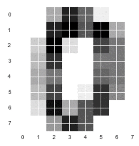
The array represents a probability for every single digit, which means that there is a 92% chance that the digit in the preceding screenshot is a 0 (which it is). Note how the next highest probability is for a 9, which makes sense because 9 and 0 have similar shapes (ovular).

Neural networks do have a major flaw. If left alone, they have a very high variance. To see this, let's run the exact same code as the preceding one and train the exact same type of neural network on the exact same data, as illustrated:

# Do it again and see the difference in error 
fnn = buildNetwork( training_data.indim, 64, training_data.outdim, outclass=SoftmaxLayer ) 
trainer = BackpropTrainer( fnn, dataset=training_data, momentum=0.1, learningrate=0.01 , verbose=True, weightdecay=0.01)  
 
# change the number of eopchs to try to get better results! 
trainer.trainEpochs (10) 
print ('Percent Error on Test dataset: ' ,  
        percentError( trainer.testOnClassData ( 
           dataset=test_data ) 
           , test_data['class'] ) )
 
accuracy = 1 - .0645879732739 
accuracy 
0.93541 

See how just rerunning the model and instantiating different weights made the network turn out to be different than before? This is a symptom of being a high variance model. In addition, neural networks generally require many training samples in order to combat the high variances of the model and also require a large amount of computation power to work well in production environments.