To get started in Azure Databricks, we have to set up our first cluster. This will spin up (initialize) resources running the Azure Databricks Runtime Environment (including Spark). This is where all of the action takes place. Whenever we run code in our notebooks, the code is sent to our cluster to actually run it. This means that no code will ever actually run on our local machine. This is great for many reasons, one of the main ones being that it provides data scientists with sub-optimal equipment at home/work a chance to use production-quality resources for a fraction of the cost!

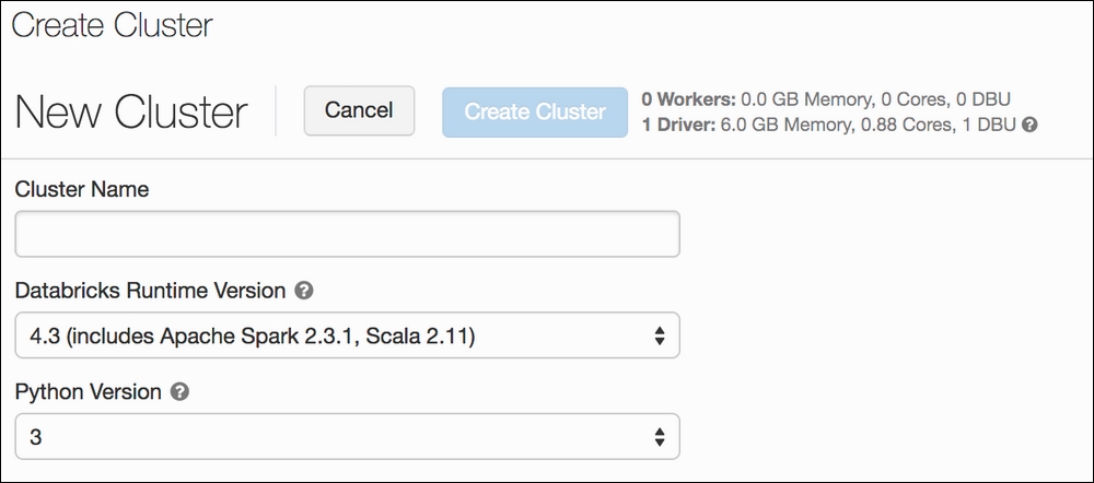
To set up a cluster, navigate to the Clusters option on the left-hand pane and click on Create cluster. There, you will see a form with three basic pieces of information: Cluster Name, Azure Databricks Runtime Version, and Python Version. Make your cluster name whatever your heart desires. Try to use the most recent Azure Databricks version (this is the default) and select Python version 3. Once that's finished, click Create cluster again and you are done.

The page should look something like this:

Once we have a cluster, it is time to set up a notebook. This can be done from the home page. When creating a new notebook, all we have to do is select the language we wish to use (Python for now, but more are available). The notebooks in Azure Databricks are nearly identical to Jupyter notebooks in functionality and use (nifty!). This comes in handy for data scientists who are used to this environment:

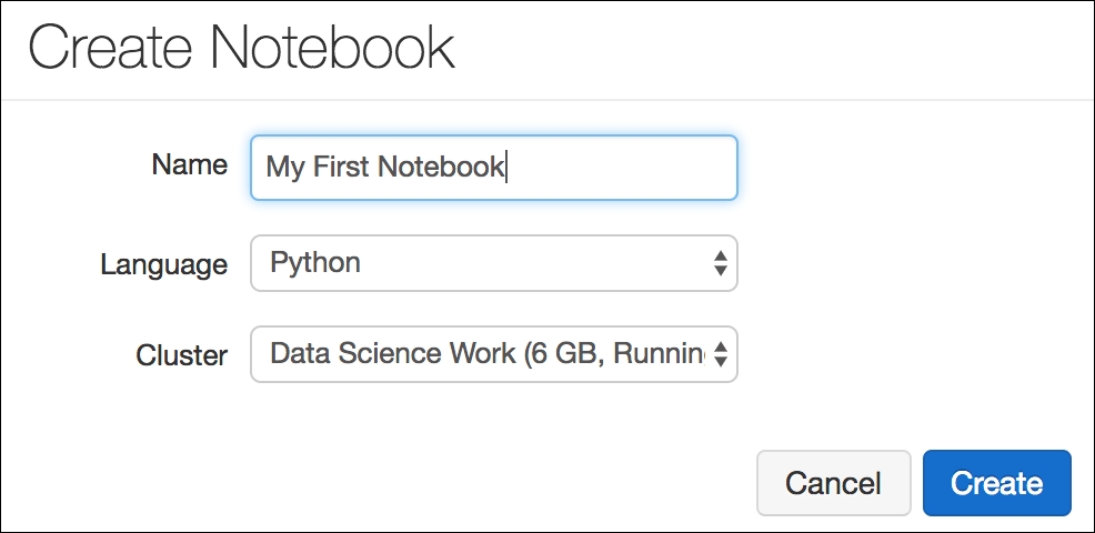
Creating a notebook is even easier than spinning up a new cluster. All of the code that we write in here will be run on our cluster and not on our local machine

Once we have our cluster up and running and we are able to create notebooks, it is time to jump right into using the Azure Databricks environment and seeing first-hand how the power of Apache Spark and the Microsoft Data Environment will affect the way that we write data-driven code.

Our first case study will focus on setting up a simple notebook in Azure Databricks and running some basic data visualization and machine learning code in order to get used to the Azure Databricks environment. Azure Databricks comes with a built-in filesystem that is preloaded with data for us to use. We can upload our own files to the system (which we will do in the second case study), but for now, we will import a dataset that came pre-loaded with Azure Databricks. We will also make heavy use of the built-in Spark-based visualization tools to analyze our data to the fullest extent that we can.

The aspects of Azure Databricks that we will be highlighting in this case study include the following:

The data that we will be using involves predicting the amount of bikes being rented via a bike-share system. Our goal is to predict the usage of the system based on daily/hourly corresponding weather, time-based, and seasonal information. Let's get right to it and see our first Azure Databricks-specific programming. We can access this through the dbutils module:

# display is a reserved function in Databricks that allows us to view and manipulate Dataframes inline
# dbutils is a library full of ready-to-use datasets for us to use
# Let's start by displaying all of the directories in the main data folder 
# "databricks-datasets"

display(dbutils.fs.ls("/databricks-datasets"))

The output is a DataFrame of available folders to look in for data. Here is a snippet:

path                                         name                 size
dbfs:/databricks-datasets/README.md          README.md            976
dbfs:/databricks-datasets/Rdatasets/         Rdatasets/           0
dbfs:/databricks-datasets/SPARK_README.md    SPARK_README.md      3359
dbfs:/databricks-datasets/adult/             adult/               0
dbfs:/databricks-datasets/airlines/          airlines/            0
dbfs:/databricks-datasets/amazon/            amazon/              0
dbfs:/databricks-datasets/asa/               asa/                 0
dbfs:/databricks-datasets/atlas_higgs/       atlas_higgs/         0
dbfs:/databricks-datasets/bikeSharing/       bikeSharing/         0
dbfs:/databricks-datasets/cctvVideos/        cctvVideos/          0
dbfs:/databricks-datasets/credit-card-fraud/ credit-card-fraud/   0
dbfs:/databricks-datasets/cs100/             cs100/               0
dbfs:/databricks-datasets/cs110x/            cs110x/              0
...

Every time we run a command in our notebook, the time that it took our cluster to execute that code is shown at the bottom. For example, this code block took my cluster 0.88 seconds. In general, the format for this statement is as follows:

Command took <<elapsed_time>> -- by <<username/email>> at <<date>>, <<time>> on <<cluster_name>>

We can view the contents of a particular file:

# Let's check out the general README of the date folder by opening the markdown folder and printing out the result of "readlines"
# which is a way to print out the contents of a file
with open("/dbfs/databricks-datasets/README.md") as f:
 x = ''.join(f.readlines())

print(x)

Databricks Hosted Datasets 
========================== 
The data contained within this directory is hosted for users to build data pipelines using Apache Spark and Databricks. 

License 
-------
....

Let's take a deeper look at the bikeSharing directory:

# Let's list the contents of the directory corresponding to the data that we want to import
display(dbutils.fs.ls("dbfs:/databricks-datasets/bikeSharing/"))

Running the preceding code will list out the contents of the bikeSharing directory:

path                                                name       size
dbfs:/databricks-datasets/bikeSharing/README.md     README.md  5016
dbfs:/databricks-datasets/bikeSharing/data-001/     data-001/  0

We have a README file in markdown format and another sub-directory. In the data-001 folder, we can list out the contents and see that there are two CSV files:

# the data is given to use in both an hourly and a daily format.
display(dbutils.fs.ls("dbfs:/databricks-datasets/bikeSharing/data-001/"))

The output is as follows:

path                                                     name       size
dbfs:/databricks-datasets/bikeSharing/data-001/day.csv   day.csv    57569
dbfs:/databricks-datasets/bikeSharing/data-001/hour.csv  hour.csv   1156736

We will use the hourly format for our study. Before we do, note that there is a README in the directory that will give us context and information about the data. We can view the file by opening it and printing our line contents as we did before:

# Note that we had to change the format from dbfs:/ to /dbfs/
with open("/dbfs/databricks-datasets/bikeSharing/README.md") as f:
 x = ''.join(f.readlines())

print(x)

## Dataset 
Bike-sharing rental process is highly correlated to the environmental and seasonal settings. For instance, weather conditions, precipitation, day of week, season, hour of the day, etc. can affect the rental behaviors. The core data set is related to the two-year historical log corresponding to years 2011 and 2012 from Capital Bikeshare system, Washington D.C., USA which is publicly available in http://capitalbikeshare.com/system-data. We aggregated the data on two hourly and daily basis and then extracted and added the corresponding weather and seasonal information. Weather information are extracted from http://www.freemeteo.com. 

...

The README goes on to say that this dataset is primarily used to do regression (predicting a continuous response). We will treat the problem as a classification by bucketing our response to classes. More on this later. Let's import our data into a good old-fashioned pandas DataFrame:

# Load data into a Pandas dataframe (note that pandas, sklearn, etc come with the environment. That's pretty neat!)
import pandas

bike_data = pandas.read_csv("/dbfs/databricks-datasets/bikeSharing/data-001/hour.csv").iloc[:,1:] # remove line number

# view the dataframe
#look at the first row
bike_data.loc[0]

The output is as follows:

dteday 2011-01-01
season 1 
yr 0 mnth 1 hr 0 holiday 0 weekday 6 workingday 0 weathersit 1 temp 0.24 atemp 0.2879 hum 0.81 windspeed 0 casual 3 registered 13 cnt 16

Descriptions for each variable are in the README:

The README included in the Azure Databricks filesystem is very helpful for context and information about the datasets. Let's see how many observations we have:

# 17,379 observations
bike_data.shape

(17379, 16)

It is nice to stop and notice that everything that we have done so far (except for the Azure Databricks filesystem module) would be exactly the same if we were to do it in a normal Jupyter environment. Let's see whether our dataset has any missing data that we would have to deal with:

# no missing data, great!
 bike_data.isnull().sum()

dteday 0 
season 0 
yr 0 
mnth 0 hr 0 
holiday 0 
weekday 0 
workingday 0 
weathersit 0 
temp 0 
atemp 0 
hum 0 
windspeed 0 
casual 0
registered 0 
cnt 0

No missing data. Excellent. Let's see a quick histogram of the cnt column, as it represents the total count of bikes reserved in that hour:

# not everything will carry over, but that is ok
%matplotlib inline

bike_data.hist("cnt")

# matplotlib inline is not supported in Databricks. 
# You can display matplotlib figures using display(). For an example, see # https://docs.databricks.com/user-guide/visualizations/matplotlib-and-ggplot.html 

We get an error when we run this code, even though we have run this command in this book before. Unfortunately, matplotlib does not work exactly the same in this environment as it does in Jupyter. That is fine, though, because Azure Databricks provides a visualization tool built on top of Spark's version of a DataFrame that puts even more capabilities at our fingertips. To get access to these visualizations, we will have to first convert our pandas DataFrame to its Spark equivalent:

# converting to a Spark DataFrame allows us to make multiple types of plots using either a sample of data or the entire data population as the source
sparkDataframe = spark.createDataFrame(bike_data)

# display is a simple way to view your data either via a table or through graphs
display(sparkDataframe)

Running the preceding code yields a snippet of the Dataframe for us to inspect:

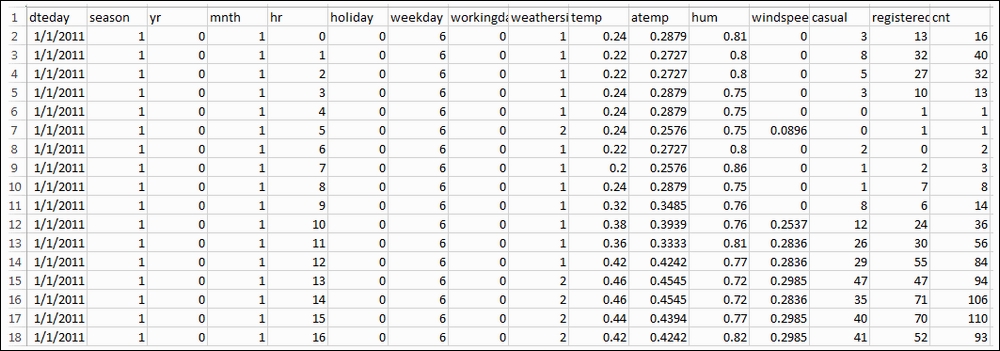
The display command shows the Spark DataFrame inline with our notebook. Azure Databricks allows for extremely powerful graphing capabilities thanks to Spark. When using the display command, on the bottom-left of the cell, a widget will appear, allowing us to graph using the data. Let's click on the Histogram:

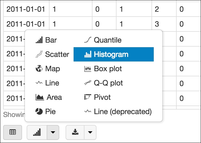
Azure Databricks offers a multitude of graphing options to get the best picture of our data

Another button will appear, called Plot Options..., which allows us to customize our graph. We can drag and drop our columns into one of three fields:

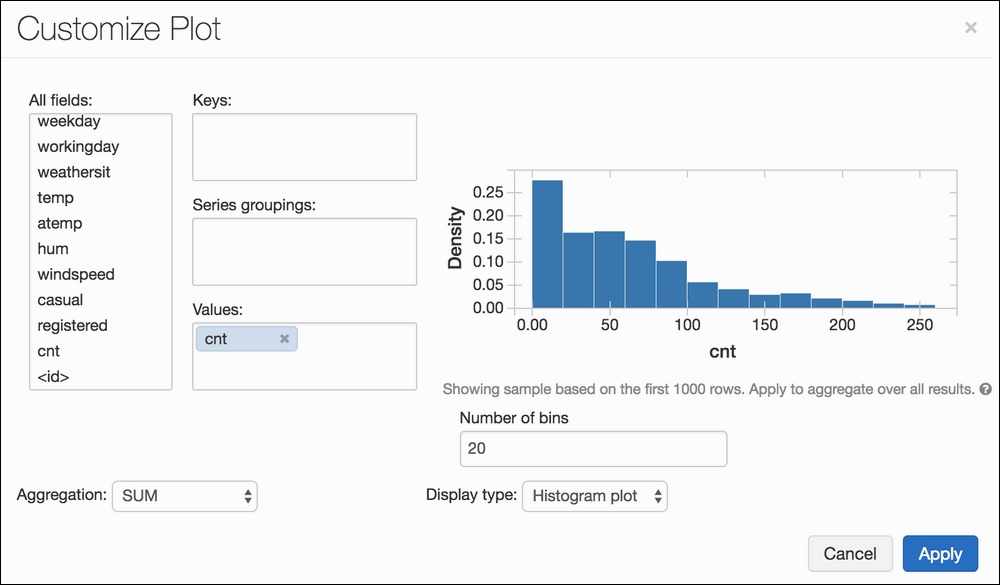
Creating a simple histogram in Azure Databricks couldn't be simpler!

We can see how easy to use the system is and that our distribution is right-skewed. Interesting! Let's try something else now. Let's say we also want to visualize the hourly usage, separated by the binary variable workingday; the idea being that we are curious to see how the total amount of bikes reserved changes by the hour and if that distribution changes depending on whether it's a working day or not. We can achieve this by selecting cnt as our value, hr as our key, and workingday as our grouping.

It should look something like this:

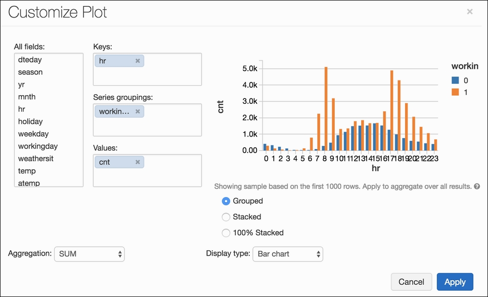
Hitting Apply will apply this to the entire dataset, instead of the first-1,000-row sample that it shows us on the right:

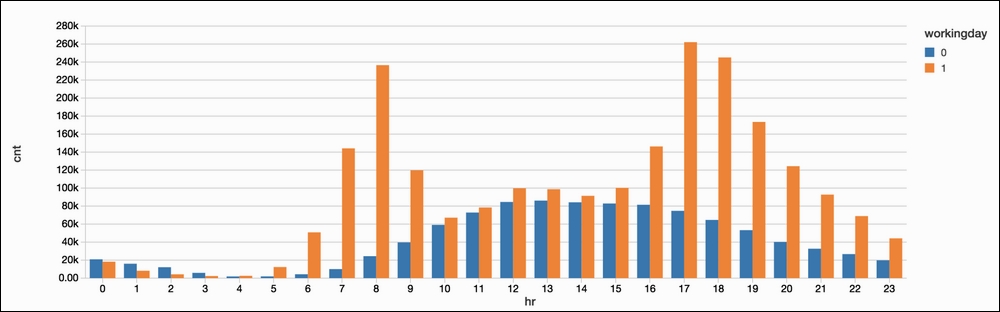
It is extremely easy to use Azure Databricks to generate beautiful and interpretable graphs based on our data. From this, we can see that bike sharing appears to be somewhat normally distributed on weekends while workdays have large spikes in the morning and evening (which makes sense).

In this dataset, there are three possible regression response candidates: casual, registered, and cnt. We will turn our problem into a classification problem by bucketing the cnt column into one of two buckets. Our response will either be 100 or fewer bikes reserved that hour (False) or over 100 (True):

# Seperate into X, and y (features and label)
# we will turn our regression problem into a classification problem by bucketing the column "cnt" as being either over 100 / 100 or under.

features, labels = bike_data[["season", "yr", "mnth", "hr", "holiday", "weekday", "workingday", "weathersit", "atemp", "hum", "windspeed"]], bike_data["cnt"] > 100

# See the distribution of our labels
labels.value_counts()

True 10344 
False 7035

Let's now create a simple function that will do a few things: take in a param choice for a random forest classifier, fit and test our model on our data, and return the results:

from sklearn.ensemble import RandomForestClassifier
from sklearn.model_selection import train_test_split
from sklearn.metrics import accuracy_score
# Create a function that will 
# 0. Take in a parameter for our Random Forest's n_estimators param# 1. Instantiate a Random Forest algorithm
# 2. Split our data into a training and testing split
# 3. Fit on our training data
# 4. evaluate on our testing data
# 5. return a tuple with the n_estimators param and corresponding accuracy

def runRandomForest(c):
 
 rf = RandomForestClassifier(n_estimators=c)
 
 # Split into train and test using sklearn.cross_validation.train_test_split
 X_train, X_test, y_train, y_test = train_test_split(features, labels, test_size=0.2, random_state=1)
 
 # Build the model
 rf.fit(X_train, y_train)
 
 # Calculate predictions and accuracy
 predictions = rf.predict(X_test)
 accuracy = accuracy_score(predictions, y_test)
 
 # return param and accuracy score
 return (c, accuracy)

This function takes in a single number as an input, sets that number as a random forest's n_estimator parameter, and returns the accuracy associated with that param choice on a train-test split:

runRandomForest(1)

(1, 0.90218642117376291)

Command took 0.13 seconds

This took a very short amount of time because we were only training a single decision tree in our forest. Let's now iteratively try a varying number of estimators and see how this affects our accuracy:

for i in [1, 10, 100, 1000, 10000]:
  print(runRandomForest(i))

(1, 0.89700805523590332) 
(10, 0.939873417721519) 
(100, 0.94677790563866515) 
(1000, 0.94677790563866515) 
(10000, 0.94792865362485612)


Command took 4.16 minutes

It took my cluster over 4 minutes to try these five n_estimator options. Most of the time was taken up by the final two options as it took a very long time to train thousands of decision trees.

Let's make use of Spark to parallelize our for loop. Every notebook has a special variable called sc that represents Spark:

# every notebook has a variable called "sc" that represents the Spark context in our cluster
sc

There are a few ways of performing this parallelization, but in general, it will look like this:

Here, we are introduced to our first Apache Spark-specific syntax. Step 1 will return a distributed dataset that is optimized for parallel computation, and we will call that dataset k. The values of k represent different possible arguments for our function, runRandomForest. Step 2 tells our cluster to run the function across our distributed dataset.

It is important to note that while Step 1 and Step 2 are Spark-specific commands, up until now, our function has not actually been sent to our cluster for execution. We have just set the stage to do so by setting up the appropriate variables. Step 3 will collect our results by running the function in parallel across the different values in k:

# 3. the collect method actually sends the five tasks to our cluster for execution

# Faster (1.5x) because we aren't doing each task one after the other. We are doing them in parallel
# This becomes much more noticeable when doing more params (we will get to this in a later case study)
results.collect()
Command took 2.73 minutes

Immediately, we can see the value of parallelizing functions using Spark. By doing nothing more than relying on Azure Databricks and Spark, we are able to perform our for loop 1.5x faster. If we use a variable in a function (like our dataset), Spark will automatically send the dataset to the workers. This is usually fine. We can send it to workers more efficiently by broadcasting it. By broadcasting data, a copy of the data is sent to our workers, which are used when running tasks. This is much more efficient when dealing with extremely large datasets with large values in them. We can rewrite our previous function using broadcast variables:

# Broadcast dataset# If we use a variable in a function, Spark will automatically send the dataset to the workers. This is usually fine.
# We can send it to workers more efficiently by broadcasting it. By broadasting data, a copy is sent to our workers which are used when running tasks. 
# For more info on broadcast variables, see the Spark programming guide. You can create a Broadcast variable using sc.broadcast().

# To access the value of a broadcast variable, you need to use .value

# broadcast the variables to our workers
featuresBroadcast = sc.broadcast(features)
labelsBroadcast = sc.broadcast(labels)

# reboot of the previous function
def runRandomForestBroadcast(c):
  
  rf = RandomForestClassifier(n_estimators=c)
    
  # Split into train and test using sklearn.cross_validation.train_test_split
  # ** This part of the function is the only difference from the previous version **
  X_train, X_test, y_train, y_test = train_test_split(featuresBroadcast.value, labelsBroadcast.value, test_size=0.2, random_state=1)
    # Build the model
  rf.fit(X_train, y_train)
    
  # Calculate predictions and accuracy
  predictions = rf.predict(X_test)
  accuracy = accuracy_score(predictions, y_test)
 
  return (c, accuracy)

Once our new function using broadcast variables is complete, running it in parallel is no different:

# set up 5 tasks in our Spark Cluster
k = sc.parallelize([1, 10, 100, 1000, 10000])
# map our function to our five tasks
results = k.map(runRandomForestBroadcast)

# the real work begins here.
results.collect()

The timing is not very different from our last run with non-broadcast data. This is because our data and logic are not large enough to see a noticeable difference yet. Once done with our variables, we can unpersist (unbroadcast) them like so:

# Since we are done with our broadcast variables, we can clean them up.
# (This will happen automatically, but we can make it happen earlier by explicitly unpersisting the broadcast variables.

featuresBroadcast.unpersist()
labelsBroadcast.unpersist()

Hyperparameter tuning would be very difficult to do if you wanted to do a grid search across multiple parameters and multiple options. We could enhance our function in order to accommodate this; however, it would be better to rely on existing frameworks in scikit-learn to do so. We will see how to remedy this conundrum in a later case study.

We can see how we can utilize Databrick's easy-to-use environment, clusters, and notebooks in order to enhance our data analysis and machine learning with minimal changes to our coding style. In the next case study, we will examine Spark's scalable machine learning library, MLlib, for optimized machine learning speed.

Our second case study will focus on predicting credit card fraud and will make use of MLlib, Apache Spark's scalable machine learning library. MLlib comes standard with our Azure Databricks environment and allows us to write scalable machine learning code. This case study will focus on MLlib syntax while we draw parallels (no pun intended) to its scikit-learn cousins.

The aspects of Azure Databricks that we will be highlighting in this case study include these:

The data in question is predicting credit card fraud. The data represents credit card transactions and contains 28 anonymized continuous features (called V1 .. V28) plus the amount that the transaction was for and the time at which the transaction occurred. We will not dive too deeply into feature engineering in this case study, but will focus mainly on using the MLlib modules that come with Azure Databricks to predict the response label (which is a binary variable). Let's get right into it and start by importing a CSV that we have uploaded using the Azure Databricks data import feature:

# File location and type
# This dataset also exists in the DBFS of Databricks. This is just to show how to import a CSV that has been previously uploaded so that
# you can upload your own!

file_location = "/FileStore/tables/creditcard.csv"
file_type = "csv"

# CSV options
# will automatically cast columns as appropiate types (float, string, etc)
infer_schema = "true"
first_row_is_header = "true"
delimiter = ","

# read a csv file and convert to a Spark dataframe
df = spark.read.format(file_type) 
 .option("inferSchema", infer_schema) 
 .option("header", first_row_is_header) 
 .option("sep", delimiter) 
 .load(file_location)

# show us the Spark Dataframe
display(df)

Our goal is to build a pipeline that will do this:

Phew. That's a lot, so let's go one step at a time. The following code block will handle Step 1, Step 2, and Step 3 by setting up a pipeline with three steps in it:

# import the pipeline module from pyspark
from pyspark.ml import Pipeline
from pyspark.ml.feature import VectorAssembler, StandardScaler, StringIndexer
# will hold the steps of our pipeline
stages = []

The first stage of our pipeline will assemble the features that we want to use in our machine learning procedure. Let's use all 28 entries from the anonymized data (V1 - V28) plus the amount column. For this case study, we will not use the time column:

# Transform all features into a vector using VectorAssembler
# create list of ["V1", "V2", "V3", ...]
numericCols = ["V{}".format(i) for i in range(1, 29)]

# Add "Amount" to the list of features
assemblerInputs = numericCols + ["Amount"]

# VectorAssembler acts like scikit-learn's "FeatureUnion" to put together the feature columns and adding the label "features"
assembler = VectorAssembler(inputCols=assemblerInputs, outputCol="features")

# add the VectorAssembler to the stages of our MLLib Pipeline
stages.append(assembler)

The second stage of our pipeline will take the assembled features and scale them:

# MLLib's StandardScaler acts like scikit-learn's StandardScaler
scaler = StandardScaler(inputCol="features", outputCol="scaledFeatures",
 withStd=True, withMean=True)
# add StandardScaler to our pipeline
stages.append(scaler)

Once we've gathered our features and scaled them, the final step of our pipeline encodes our class label to ensure consistency:

# Convert label into label indices using the StringIndexer (like scikit-learn's LabelEncoder)
label_stringIdx = StringIndexer(inputCol="Class", outputCol="label")
# add the StringIndexer to our pipeline
stages.append(label_stringIdx)

That was a lot, but note that every step of the pipeline has a scikit-learn equivalent. As a data scientist, the most important thing to remember is that as long as you know the theory and the proper steps of data science and machine learning, you can transfer your skills across many languages, platforms, and technologies. Now that we have created our list of three stages, let's instantiate a pipeline object:

# create our pipeline with three stages
pipeline = Pipeline(stages=stages)

To make sure that we are training a model that is able to predict unseen cases, we should split up our data into a training and testing set, and fit our pipeline to the training set while using the trained pipeline to transform the testing set:

# We need to split our data into training and test sets. This is like scikit-learn's train_test_split function
# We will also set a random number seed for reproducibility

(trainingData, testData) = df.randomSplit([0.7, 0.3], seed=1)
print(trainingData.count())
print(testData.count())
199470  # elements in the training set
85337  # elements in the testing set

Let's now fit our pipeline to the training set. This will learn the features as well as the parameters to scale future unseen testing data:

# fit and transform to our training data
pipelineModel = pipeline.fit(trainingData)
trainingDataTransformed = pipelineModel.transform(trainingData)

If we take a look at our DataFrame, we will notice that we have three new columns: features, scaledFeatures, and label. These three columns were added by our pipeline and those names can be found exactly in the preceding code where we set the three stages of the pipeline. Note that the data types of the features and scaledFeatures column are vector. This indicates that they represent observations to be learned by our machine learning model in the future:

# note the new columns "features", "scaledFeatures", and "label" at the end
trainingDataTransformed

Time:decimal(10,0)
V1:double
V2:double
V3:double
V4:double
V5:double
V6:double
V7:double
V8:double
V9:double
V10:double
V11:double
V12:double
V13:double
V14:double
V15:double
V16:double
V17:double
V18:double
V19:double
V20:double
V21:double
V22:double
V23:double
V24:double
V25:double
V26:double
V27:double
V28:double
Amount:double
Class:integer
features:udt
scaledFeatures:udt
label:double

Just like we do in scikit-learn, we will have to import out logistic regression model, instantiate it, and fit it to our training data:

# Import the logistic regression module from pyspark
from pyspark.ml.classification import LogisticRegression

# Create initial LogisticRegression model
lr = LogisticRegression(labelCol="label", featuresCol="scaledFeatures")

# Train model with Training Data
lrModel = lr.fit(trainingDataTransformed)

This process should look very familiar to us as it is nearly identical to scikit-learn. The main difference is that when we instantiate our model, we have to tell the object the names of the label and features, instead of feeding the features and label separately into the fit method (like we do in scikit-learn).

Once we fit our model, we can transform and gather predictions from our testing data:

# transform (not fit) to the testing data
testDataTransformed = pipelineModel.transform(testData)

# run our logistic regression over the transformed testing set
predictions = lrModel.transform(testDataTransformed)

Transforming our testing data using logistic regression will actually add three new columns (like the pipeline did). We can see this by running this:

predictions:
Time: decimal(10,0)
V1: double
V2: double
V3: double
V4: double
V5: double
V6: double
V7: double
V8: double
V9: double
V10: double
V11: double
V12: double
V13: double
V14: double
V15: double
V16: double
V17: double
V18: double
V19: double
V20: double
V21: double
V22: double
V23: double
V24: double
V25: double
V26: double
V27: double
V28: double
Amount: double
Class: integer
features: udt
scaledFeatures: udt
label: double
rawPrediction: udt
probability: udt
prediction: double

Let's take a look at the label column as well as two of the new columns, probability and prediction. We can do this by invoking the filter method of the Spark DataFrame:

selected = predictions.select("label", "prediction", "probability")
display(selected)

The output is as follows:

label prediction probability
0     0          [1,2,[],[0.9998645390717447,0.000135460928255428]]
0          [1,2,[],[0.9998821292706751,0.00011787072932487872]]
0     0          [1,2,[],[0.9994714991454193,0.000528500854580697]]
0     0          [1,2,[],[0.9991193503498385,0.0008806496501614437]]
0     0          [1,2,[],[0.9997043818469743,0.00029561815302580084]]
0     0          [1,2,[],[0.9998106820888389,0.00018931791116114655]]
0     0          [1,2,[],[0.9995735877526569,0.0004264122473429876]]
...

The label and prediction columns show each observation's ground truth and our model's estimate, while the probability column holds a vector that contains the predicted probability (think scikit-learn's predict_proba functionality). Let's now bring in PySpark's metric evaluation module in order to get some basic metrics. we will start with BinaryClassificationEvaluator, which can tell us the testing AUC (area under the ROC curve):

# like scikit-learn's metric module
from pyspark.ml.evaluation import BinaryClassificationEvaluator

# Evaluate model using either area under Precision Recall curev or the area under the ROC
evaluator = BinaryClassificationEvaluator(rawPredictionCol="rawPrediction", metricName="areaUnderROC")
evaluator.evaluate(predictions)

0.984986959421

This is helpful, but we also want some of the more familiar and interpretable metrics such as accuracy, precision, recall, and more. We can get these using PySpark's MulticlassMetrics module:

# Get some deeper metrics out of our predictions
from pyspark.mllib.evaluation import MulticlassMetrics

# must turn DF into RDD (Resilient Distributed Dataset)
predictionAndLabels = predictions.select("label", "prediction").rdd.map(tuple)

# instantiate a MulticlassMetrics object
metrics = MulticlassMetrics(predictionAndLabels)

# Overall statistics
accuracy = metrics.accuracy
precision = metrics.precision()
recall = metrics.recall()
f1Score = metrics.fMeasure()
print("Summary Stats")
print("Accuracy = %s" % accuracy)
print("Precision = %s" % precision)
print("Recall = %s" % recall)
print("F1 Score = %s" % f1Score)

The output is as follows:

Summary Stats 
Accuracy = 0.999203159239 
Precision = 0.999203159239 
Recall = 0.999203159239 
F1 Score = 0.999203159239

Great! We can also calculate our true positive rate, false negative rate, and other by using the predictions vector. This will give us a better sense of how our machine learning model performs on particular examples of positive and negative fraud cases:

tp = predictions[(predictions.label == 1) & (predictions.prediction == 1)].count()
tn = predictions[(predictions.label == 0) & (predictions.prediction == 0)].count()
fp = predictions[(predictions.label == 0) & (predictions.prediction == 1)].count()
fn = predictions[(predictions.label == 1) & (predictions.prediction == 0)].count()

print ("True Positives:", tp)
print ("True Negatives:", tn)
print ("False Positives:", fp)
print ("False Negatives:", fn)

The output is as follows:

True Positives: 93 
True Negatives: 85176 
False Positives: 18 
False Negatives: 50

Let's consider this our baseline logistic regression model and try to optimize our results by tweaking our logistic regression parameters.

# explain the parameters that are included in MLLib's Logistic Regression
print(lr.explainParams())

aggregationDepth: suggested depth for treeAggregate (>= 2). (default: 2) elasticNetParam: the ElasticNet mixing parameter, in range [0, 1]. For alpha = 0, the penalty is an L2 penalty. For alpha = 1, it is an L1 penalty. (default: 0.0)
family: The name of family which is a description of the label distribution to be used in the model. Supported options: auto, binomial, multinomial (default: auto) featuresCol: features column name. (default: features, current: scaledFeatures) fitIntercept: whether to fit an intercept term. (default: True) 
labelCol: label column name. (default: label, current: label)
....

# pyspark's version of GridSearchCV
from pyspark.ml.tuning import ParamGridBuilder, CrossValidator

# Create ParamGrid for Cross Validation
paramGrid = (ParamGridBuilder()
 .addGrid(lr.regParam, [0.0, 0.01, 0.5, 2.0])
 .addGrid(lr.elasticNetParam, [0.0, 0.5, 1.0])
 .addGrid(lr.maxIter, [5, 10]).build())


# Create 5-fold CrossValidator that can also test multiple parameters (like scikit-learn's GridSearchCV)
cv = CrossValidator(estimator=lr, estimatorParamMaps=paramGrid, evaluator=evaluator, numFolds=5)

# Run cross validations on our cluster
cvModel = cv.fit(trainingDataTransformed)
# this will likely take a fair amount of time because of the amount of models that we're creating and testing

# extract the weights from our model
weights = cvModel.bestModel.coefficients
# convert from numpy type to float
weights = [[float(w)] for w in weights]
weightsDF = sqlContext.createDataFrame(weights, ["Feature Weight"])
display(weightsDF)

Feature Weight

-0.009310428799214699
0.024089617982041803
-0.07660344812402071
0.13879375587420806
0.03389644146602658
-0.03197804822203382
-0.026671134727093863
-0.05963860645699601
-0.07157334685249503
-0.12739634200985744
0.11271203988538568
-0.16991941687681994
-0.022382161065846975
-0.2967372927422323
-0.002525484797586701
-0.08661888759753078
-0.09428351861530046
-0.010145267312697291
0.000474661023205239
0.003985147929831393
0.031230406955806467
0.011362000753207976
-0.014548646956536248
-0.011270335506048019
-0.004390342109545349
0.008722583938741943
0.01390573346423987
0.014176539525542918
0.021489763526114244

# Use test set to get the best params
predictions = cvModel.transform(testDataTransformed)

# must turn DF into RDD (Resilient Distributed Dataset)
predictionAndLabels = predictions.select("label", "prediction").rdd.map(tuple)

metrics = MulticlassMetrics(predictionAndLabels)

# Overall statistics
accuracy = metrics.accuracy
precision = metrics.precision()
recall = metrics.recall()
f1Score = metrics.fMeasure()
print("Summary Stats")
print("Accuracy = %s" % accuracy)
print("Precision = %s" % precision)
print("Recall = %s" % recall)
print("F1 Score = %s" % f1Score)

Summary Stats 
Accuracy = 0.998839893598 
Precision = 0.998839893598 
Recall = 0.998839893598 
F1 Score = 0.998839893598

tp = predictions[(predictions.label == 1) & (predictions.prediction == 1)].count()
tn = predictions[(predictions.label == 0) & (predictions.prediction == 0)].count()
fp = predictions[(predictions.label == 0) & (predictions.prediction == 1)].count()
fn = predictions[(predictions.label == 1) & (predictions.prediction == 0)].count()

print "True Positives:", tp
print "True Negatives:", tn
print "False Positives:", fp
print "False Negatives:", fn
# False positive went from 18 to 16 (win) but False Negative jumped to 83 (opposite of win)

True Positives: 67 
True Negatives: 85178 
False Positives: 16 
False Negatives: 76

How to add Python libraries to your cluster

Up until now, all of the packages that we have used come with the Azure Databricks environment. Now we need to add a new package, called spark_sklearn. To add a third-party package to our Azure Databricks cluster, we simply click on Import Library from our main dashboard, and we will see a window like the following:

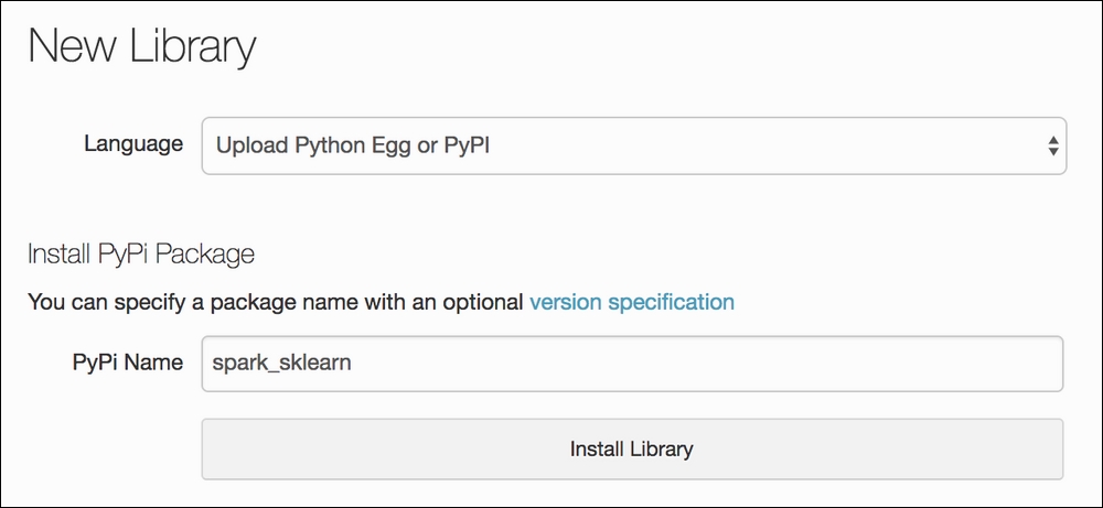
Type in any package that you wish to use in the PyPi Name field

We simply type in spark_sklearn, hit Install Library, and we are done! The cluster will now let us import the library from any existing or new notebook. Now, spark_sklearn is a handy tool that allows the use of some scikit-learn packages with the backend swapped out for PySpark. This means that we can use existing code that we have already written, and only have to tweak it slightly to make it compatible with Spark.

from sklearn import datasets
from sklearn.ensemble import RandomForestClassifier
from sklearn.model_selection import GridSearchCV as original_grid_search
digits = datasets.load_digits()

X, y = digits.data, digits.target

param_grid = {"max_depth": [3, None],
 "max_features": [1, 3, 10],
 "min_samples_leaf": [1, 3, 10],
 "bootstrap": [True, False],
 "criterion": ["gini", "entropy"],
 "n_estimators": [10, 100, 1000]}
gs = original_grid_search(RandomForestClassifier(), param_grid=param_grid)
gs.fit(X, y)

gs.best_params_, gs.bestscore

({'bootstrap': False,   
'criterion': 'gini',   
'max_depth': None,   
'max_features': 3,   
'min_samples_leaf': 1,   
'n_estimators': 1000},  
0.95436839176405119)

Command took 24.69 minutes 

# the new gridsearch module
from spark_sklearn import GridSearchCV as spark_grid_search

# the only difference is passing in the SparkContext objecr as the first parameter of the grid searchgs = spark_grid_search(sc, RandomForestClassifier(), param_grid=param_grid)
gs.fit(X, y)

gs.best_params_, gs.bestscore

({'bootstrap': False,
'criterion': 'gini',   
'max_depth': None,   
'max_features': 3,   
'min_samples_leaf': 1,   
'n_estimators': 100}, 
0.95436839176405119)

Command took 5.29 minute