
Ensemble learning, or ensembling, is the process of combining multiple predictive models to produce a supermodel that is more accurate than any individual model on its own:
Imagine that we are working on a binary classification problem (predicting either 0 or 1):
# ENSEMBLING

import numpy as np

# set a seed for reproducibility
np.random.seed(12345)

# generate 2000 random numbers (between 0 and 1) for each model, representing 2000 observations
mod1 = np.random.rand(2000)
mod2 = np.random.rand(2000)
mod3 = np.random.rand(2000)
mod4 = np.random.rand(2000)
mod5 = np.random.rand(2000)
Now, we simulate five different learning models, and each has about a 70% accuracy, as follows:
# each model independently predicts 1 (the "correct response") if random number was at least 0.4
preds1 = np.where(mod1 > 0.4, 1, 0)
preds2 = np.where(mod2 > 0.4, 1, 0)
preds3 = np.where(mod3 > 0.4, 1, 0)
preds4 = np.where(mod4 > 0.4, 1, 0)
preds5 = np.where(mod5 > 0.4, 1, 0)
print(preds1.mean()) 0.596print (preds2.mean()) 0.6065print (preds3.mean()) 0.591print (preds4.mean()) 0.5965print( preds5.mean()) # 0.611
# Each model has an "accuracy of around 60% on its own
Now, let's apply my degrees in magic. Er... sorry, math:
# average the predictions and then round to 0 or 1
ensemble_preds = np.round((preds1 + preds2 + preds3 + preds4 + preds5)/5.0).astype(int)
ensemble_preds.mean()
The output is as follows:
0.674
As you add more models to a voting process, the probability of errors will decrease; this is known as Condorcet's jury theorem.
Crazy, right?
For ensembling to work well in practice, the models must have the following characteristics:
- Accuracy: Each model must at least outperform the null model
- Independence: A model's prediction process is not affected by another model's prediction process
If you have a bunch of individually OK models, the edge case mistakes made by one model are probably not going to be made by the other models, so the mistakes will be ignored when combining the models.
There are the following two basic methods for ensembling:
- Manually ensemble your individual models by writing a good deal of code
- Use a model that ensembles for you
We're going to look at a model that ensembles for us. To do this, let's take a look at decision trees again.
Decision trees tend to have low bias and high variance. Given any dataset, the tree can keep asking questions (making decisions) until it is able to nitpick and distinguish between every single example in the dataset. It could keep asking question after question until there is only a single example in each leaf (terminal) node. The tree is trying too hard, growing too deep, and just memorizing every single detail of our training set. However, if we started over, the tree could potentially ask different questions and still grow very deep. This means that there are many possible trees that could distinguish between all elements, which means the higher variance. It is unable to generalize well.
In order to reduce the variance of a single tree, we can place a restriction on the number of questions asked in a tree (the max_depth parameter) or we can create an ensemble version of decision trees, called random forests.
The primary weakness of decision trees is that different splits in the training data can lead to very different trees. Bagging is a general purpose procedure to reduce the variance of a machine learning method but is particularly useful for decision trees.
Bagging is short for Bootstrap aggregation, which means the aggregation of Bootstrap samples. What is a Bootstrap sample?
A Bootstrap sample is a smaller sample that is "bootstrapped" from a larger sample. Bootstrapping is a type of resampling where large numbers of smaller samples of the same size are repeatedly drawn, with replacement, from a single original sample:
# set a seed for reproducibility
np.random.seed(1)

# create an array of 1 through 20
nums = np.arange(1, 21)
print (nums).
The output is as follows:
[ 1  2  3  4  5  6  7  8  9 10 11 12 13 14 15 16 17 18 19 20]
# sample that array 20 times with replacement
np.random.choice(a=nums, size=20, replace=True)
The preceding command will create a bootstrapped sample as follows:
 [ 6 12 13  9 10 12  6 16  1 17  2 13  8 14  7 19  6 19 12 11]
# This is our bootstrapped sample notice it has repeat variables!
So, how does bagging work for decision trees?
- Grow B trees using Bootstrap samples from the training data
- Train each tree on its Bootstrap sample and make predictions
- Combine the predictions:
- Average the predictions for regression trees
- Take a vote for classification trees
The following are a few things to note:
- Each Bootstrap sample should be the same size as the original training set
- B should be a large enough value that the error seems to have stabilized
- The trees are grown intentionally deep so that they have low bias/high variance
The reason we grow the trees intentionally deep is that the bagging inherently increases predictive accuracy by reducing the variance, similar to how cross-validation reduces the variance associated with estimating our out-of-sample error.
Random forests are a variation of bagged trees.
However, when building each tree, each time we consider a split between the features, a random sample of m features is chosen as split candidates from the full set of p features. The split is only allowed to be one of those m features:
- A new random sample of features is chosen for every single tree at every single split
- For classification, m is typically chosen to be the square root of p
- For regression, m is typically chosen to be somewhere between p/3 and p
What's the point?
Suppose there is one very strong feature in the dataset. When using decision (or bagged) trees, most of the trees will use that feature as the top split, resulting in an ensemble of similar trees that are highly correlated with each other.
If our trees are highly correlated with each other, then averaging these quantities will not significantly reduce variance (which is the entire goal of ensembling). Also, by randomly leaving out candidate features from each split, random forests reduce the variance of the resulting model.
Random forests can be used in both classification and regression problems and can be easily used in scikit-learn. Let's try to predict MLB salaries based on statistics about the player, as shown:
# read in the data
url = '../data/hitters.csv'

hitters = pd.read_csv(url)

# remove rows with missing values
hitters.dropna(inplace=True)

# encode categorical variables as integers
hitters['League'] = pd.factorize(hitters.League)[0]
hitters['Division'] = pd.factorize(hitters.Division)[0]
hitters['NewLeague'] = pd.factorize(hitters.NewLeague)[0]

# define features: exclude career statistics (which start with "C") and the response (Salary)
feature_cols = [h for h in hitters.columns if h[0] != 'C' and h != 'Salary']


# define X and y
X = hitters[feature_cols]
y = hitters.Salary
Let's try and predict the salary first using a single decision tree, as illustrated:
from sklearn.tree import DecisionTreeRegressor

# list of values to try for max_depth
max_depth_range = range(1, 21)

# list to store the average RMSE for each value of max_depth
RMSE_scores = []

# use 10-fold cross-validation with each value of max_depth
from sklearn.cross_validation import cross_val_score
for depth in max_depth_range:
    treereg = DecisionTreeRegressor(max_depth=depth, random_state=1)
    MSE_scores = cross_val_score(treereg, X, y, cv=10, scoring='mean_squared_error')
    RMSE_scores.append(np.mean(np.sqrt(-MSE_scores)))

# plot max_depth (x-axis) versus RMSE (y-axis)
plt.plot(max_depth_range, RMSE_scores)
plt.xlabel('max_depth')
plt.ylabel('RMSE (lower is better)') 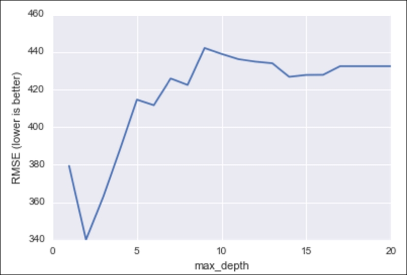
RMSE for decision tree models against the max depth of the tree (complexity)
Let's do the same thing, but this time with a random forest:
from sklearn.ensemble import RandomForestRegressor


# list of values to try for n_estimators
estimator_range = range(10, 310, 10)

# list to store the average RMSE for each value of n_estimators
RMSE_scores = []

# use 5-fold cross-validation with each value of n_estimators (WARNING: SLOW!)
for estimator in estimator_range:
    rfreg = RandomForestRegressor(n_estimators=estimator, random_state=1)
    MSE_scores = cross_val_score(rfreg, X, y, cv=5, scoring='mean_squared_error')
    RMSE_scores.append(np.mean(np.sqrt(-MSE_scores)))


# plot n_estimators (x-axis) versus RMSE (y-axis)
plt.plot(estimator_range, RMSE_scores)
plt.xlabel('n_estimators')
plt.ylabel('RMSE (lower is better)') 
RMSE for random forest models against the max depth of the tree (complexity)
Note already the y-axis; our RMSE is much lower on an average! See how we can obtain a major increase in predictive power using random forests.
In random forests, we still have the concept of important features, like we had in decision trees:
# n_estimators=150 is sufficiently good
rfreg = RandomForestRegressor(n_estimators=150, random_state=1)
rfreg.fit(X, y)
# compute feature importances
pd.DataFrame({'feature':feature_cols, 'importance':rfreg.feature_importances_}).sort('importance', ascending = False) 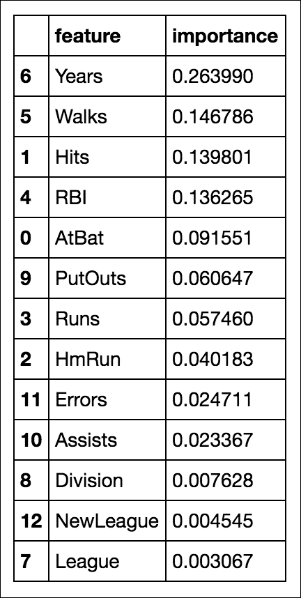
So, it looks like the number of years the player has been in the league is still the most important feature when deciding that player's salary.