A discrete random variable only takes on a countable number of possible values, such as the outcome of a dice roll, as shown here:

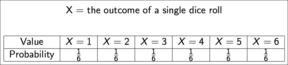
Note how I use a capital X to define the random variable. This is a common practice. Also note how the random variable maps a probability to each individual outcome. Random variables have many properties, two of which are their expected value and the variance. We will use a probability mass function (PMF) to describe a discrete random variable.

They take on the following appearance:

So, for a dice roll, P(X = 1) = 1/6 and P(X = 5) = 1/6.

Consider the following examples of discrete variables:

The expected value of a random variable defines the mean value of a long run of repeated samples of the random variable. This is sometimes called the mean of the variable.

For example, refer to the following Python code, which defines the random variable of a dice roll:

import random 
def random_variable_of_dice_roll(): 
    return random.randint(1, 7) # a range of (1,7) # includes 1, 2, 3, 4, 5, 6, but NOT 7 

This function will invoke a random variable and come out with a response. Let's roll 100 dice and average the result, as follows:

trials = [] 
num_trials = 100 
for trial in range(num_trials): 
trials.append( random_variable_of_dice_roll() ) 
print(sum(trials)/float(num_trials))  # == 3.77 

So, taking 100 dice rolls and averaging them gives us a value of 3.77! Let's try this with a wide variety of trial numbers, as illustrated here:

num_trials = range(100,10000, 10) 
avgs = [] 
for num_trial in num_trials: 
    trials = [] 
    for trial in range(1,num_trial): 
        trials.append( random_variable_of_dice_roll() ) 
    avgs.append(sum(trials)/float(num_trial)) 
 
plt.plot(num_trials, avgs) 
plt.xlabel('Number of Trials') 
plt.ylabel("Average")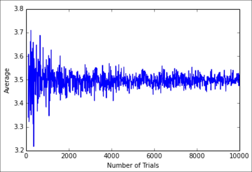 

We get the following graph:

The preceding graph represents the average dice roll as we look at more and more dice rolls. We can see that the average dice roll is rapidly approaching 3.5. If we look towards the left of the graph, we see that if we only roll a die about 100 times, then we are not guaranteed to get an average dice roll of 3.5. However, if we roll 10,000 dice one after another, we see that we would very likely expect the average dice roll to be about 3.5.

For a discrete random variable, we can also use a simple formula, shown as follows, to calculate the expected value:

Here, x_i is the i^th outcome and p_i is the i^th probability.

So, for our dice roll, we can find the exact expected value as follows:

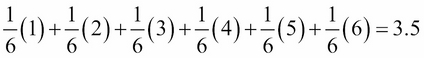
The preceding result shows us that for any given dice roll, we can expect a dice roll of 3.5. Now, obviously, that doesn't make sense because we can't get a 3.5 on a dice roll, but it does make sense when put in the context of many dice rolls. If you roll 10,000 dice, your average dice roll should approach 3.5, as shown in the graph and code previously.

The average of the expected value of a random variable is generally not enough to grasp the full idea behind the variable. For this reason, we introduce a new concept, called variance.

The variance of a random variable represents the spread of the variable. It quantifies the variability of the expected value.

The formula for the variance of a discrete random variable is expressed as follows:

x i and p i represent the same values as before and represents the expected value of the variable. In this formula, I also mentioned the sigma of X. Sigma, in this case, is the standard deviation, which is defined simply as the square root of the variance. Let's look at a more complicated example of a discrete random variable.

Variance can be thought of like a give or take metric. If I say you can expect to win $100 from a poker hand, you might be very happy. If I append that statement with the additional detail that you might win $100, give or take $80, you now have a wide range of expectations to deal with, which can be frustrating and might make a risk-averse player more wary of joining the game. We can usually say that we have an expected value, give or take the standard deviation.

Consider that your team measures the success of a new product on a Likert scale, that is, as being in one of five categories, where a value of 0 represents a complete failure and 4 represents a great success. They estimate that a new project has the following chances of success based on user testing and the preliminary results of the performance of the product.

We first have to define our random variable.

Let the X random variable represent the success of our product. X is indeed a discrete random variable because the X variable can only take on one of five options: 0, 1, 2, 3, or 4.

The following is the probability distribution of our random variable, X. Note how we have a column for each potential outcome of X and, following each outcome, we have the probability that that particular outcome will be achieved:

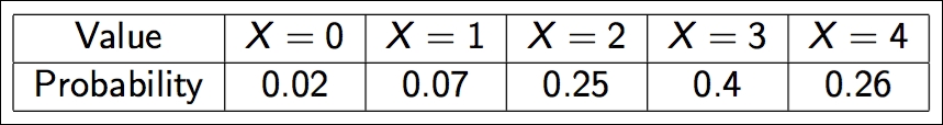
For example, the project has a 2% chance of failing completely and a 26% chance of being a great success! We can calculate our expected value as follows:

E[X] = 0(0.02) + 1(0.07) + 2(0.25) + 3(0.4) + 4(0.26) = 2.81

This number means that the manager can expect a success of about 2.81 out of this project. Now, by itself, that number is not very useful. Perhaps, if given several products to choose from, an expected value might be a way to compare the potential successes of several products. However, in this case, when we have but the one product to evaluate, we will need more.

Now, let's check the variance, as shown here:

Variance=V[X]=σX2 = (xi −μX)2pi = (0 − 2.81)2(0.02) + (1 − 2.81)2(0.07)+(2 − 2.81)2(0.25) + (3 − 2.81)2(0.4) + (4 − 2.81)2(0.26) = .93

Now that we have both the standard deviation and the expected value of the score of the project, let's try to summarize our results. We could say that our project will have an expected score of 2.81 plus or minus 0.96, meaning that we can expect something between 1.85 and 3.77.

So, one way we can address this project is that it is probably going to have a success rating of 2.81, give or take about a point.

You might be thinking, wow, Sinan, so at best the project will be a 3.8 and at worst it will be a 1.8?. Not quite.

It might be better than a 4 and it might also be worse than a 1.8. To take this one step further, let's calculate the following:

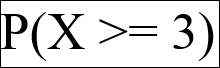
First, take a minute and convince yourself that you can read that formula to yourself. What am I asking when I am asking for P(X >= 3)? Honestly, take a minute and figure it out.

P(X >= 3) is the probability that our random variable will take on a value at least as big as 3. In other words, what is the chance that our product will have a success rating of 3 or higher? To calculate this, we can calculate the following:

P(X >= 3) = P(X = 3) + P(X = 4) = .66 = 66%

This means that we have a 66% chance that our product will rate as either a 3 or a 4.

Another way to calculate this would be the conjugate way, as shown here:

P(X >= 3) = 1 - P(X < 3)

Again, take a moment to convince yourself that this formula holds up. I am claiming that to find the probability that the product will be rated at least a 3 is the same as 1 minus the probability that the product will receive a rating below 3. If this is true, then the two events (X >=3 and X < 3) must complement one another.

This is obviously true! The product can be either of the following two options:

Let's check our math:

P(X < 3) = P(X = 0) + P(X = 1) + P(X = 2)

= 0.02 + 0.07 + 0.25

= .0341 - P(X < 3)

= 1 - .34

= .66

= P( x >= 3)

It checks out!

The first type of discrete random variable we will look at is called a binomial random variable. With a binomial random variable, we look at a setting in which a single event happens over and over and we try to count the number of times the result is positive.

Before we can understand the random variable itself, we must look at the conditions in which it is even appropriate.

A binomial setting has the following four conditions:

A binomial random variable is a discrete random variable, X, that counts the number of successes in a binomial setting. The parameters are n = the number of trials and p = the chance of success of each trial.

Example: Fundraising meetings

A start-up is taking 20 VC meetings to fund and count the number of offers they receive.

The PMF for a binomial random variable is as follows:

Example: Restaurant openings

A new restaurant in a town has a 20% chance of surviving its first year. If 14 restaurants open this year, find the probability that exactly four restaurants survive their first year of being open to the public.

First, we should prove that this is a binomial setting:

Here, we have our two parameters of n = 14 and p = 0.2. So, we can now plug these numbers into our binomial formula, as shown here:

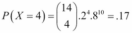
So, we have a 17% chance that exactly 4 of these restaurants will be open after a year.

Example: Blood types

A couple has a 25% chance of a having a child with type O blood. What is the chance that three of their five kids have type O blood?

Let X = the number of children with type O blood with n = 5 and p = 0.25, as shown here:

We can calculate this probability for the values of 0, 1, 2, 3, 4, and 5 to get a sense of the probability distribution:

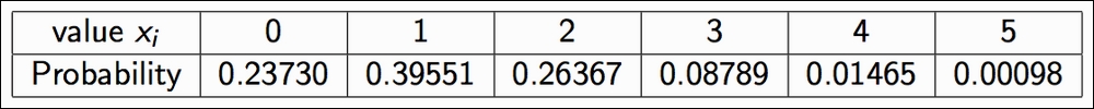
From here, we can calculate an expected value and the variance of this variable:

So, this family can expect to have probably one or two kids with type O blood!

What if we want to know the probability that at least three of their kids have type O blood? To know the probability that at least three of their kids have type O blood, we can use the following formula for discrete random variables:

P(x>=3) =P(X=3)+P(X=4)+P(X=3) = .00098+.01465+.08789=0.103

So, there is about a 10% chance that three of their kids have type O blood.

A binomial random variable is a discrete random variable that counts the number of successes in a binomial setting. It is used in a wide variety of data-driven experiments, such as counting the number of people who will sign up for a website given a chance of conversion, or even, at a simple level, predicting stock price movements given a chance of decline (don't worry; we will be applying much more sophisticated models to predict the stock market later).

Geometric random variables

The second discrete random variable we will take a look at is called a geometric random variable. It is actually quite similar to the binomial random variable in that we are concerned with a setting in which a single event is occurring over and over. However, in the case of a geometric setting, the major difference is that we are not fixing the sample size.

We are not going into exactly 20 VC meetings as a start-up, nor are we having exactly five kids. Instead, in a geometric setting, we are modeling the number of trials we will need to see before we obtain even a single success. Specifically, a geometric setting has the following four conditions:

• The possible outcomes are either success or failure
• The outcomes of trials cannot affect the outcome of another trial
• The number of trials was not set
• The chance of success of each trial must always be p

Note that these are the exact same conditions as a binomial variable, except the third condition.

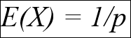
A geometric random variable is a discrete random variable, X, that counts the number of trials needed to obtain one success. The parameters are p = the chance of success of each trial and (1 − p) = the chance of failure of each trial.

To transform the previous binomial examples into geometric examples, we might do the following:

• Count the number of VC meetings that a start-up must take in order to get their first yes
• Count the number of coin flips needed in order to get a head (yes, I know it's boring, but it's a solid example!)

The formula for the PMF is as follows:

Both the binomial and geometric settings involve outcomes that are either successes or failures. The big difference is that binomial random variables have a fixed number of trials, denoted as n. Geometric random variables do not have a fixed number of trials. Instead, geometric random variables model the number of samples needed in order to obtain the first successful trial, whatever success might mean in those experimental conditions.

Example: Weather

There is a 34% chance that it will rain on any day in April. Find the probability that the first day of rain in April will occur on April 4.

Let X = the number of days until it rains (success) with p = 0.34 and (1 − p) = 0.66.

Lets' work it out:

The probability that it will rain by the April 4 is as follows:

P(X<=4) = P(1) + P(2) + P(3) + P(4) = .34 + .22 + .14 +>1 = .8

So, there is an 80% chance that the first rain of the month will happen within the first four days.

Note

Shortcuts to geometric expected value and varianceGeometric random variables also have special calculations for the exact values of the expected values and variance. If X is a geometric random variable, then we get the following:

Poisson random variable

The third and last specific example of a discrete random variable is a Poisson random variable.

To understand why we would need this random variable, imagine that an event that we wish to model has a small probability of happening and that we wish to count the number of times that the event occurs in a certain time frame. If we have an idea of the average number of occurrences, µ, over a specific period of time, given from past instances, then the Poisson random variable, denoted by X = Poi(µ), counts the total number of occurrences of the event during that given time period.

In other words, the Poisson distribution is a discrete probability distribution that counts the number of events that occur in a given interval of time.

Consider the following examples of Poisson random variables:

• Finding the probability of having a certain number of visitors on your site within an hour, knowing the past performance of the site
• Estimating the number of cars crashes at an intersection based on past police reports

If we let X = the number of events in a given interval, and the average number of events per interval is the λ number, then the probability of observing x events in a given interval is given by the following formula:

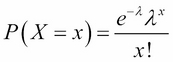
Here, e = Euler's constant (2.718....).

Example: Call center

The number of calls arriving at your call center follows a Poisson distribution at the rate of five calls per hour. What is the probability that exactly six calls will come in between 10 and 11 p.m.?

To set up this example, let's write out our given information. Let X be the number of calls that arrive between 10 and 11 p.m. This is our Poisson random variable with the mean λ = 5. The mean is 5 because we are using 5 as our previous expected value of the number of calls to come in at this time. This number could have come from the previous work on estimating the number of calls that come in every hour or specifically that come in after 10 p.m. The main idea is that we do have some idea of how many calls should be coming in, and then we use that information to create our Poisson random variable and use it to make predictions.

Continuing with our example, we have the following:

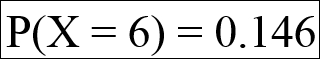
This means that there is about a 14.6% chance that exactly six calls will come between 10 and 11 p.m.

Note

Shortcuts to Poisson expected value and variance

Poisson random variables also have special calculations for the exact values of the expected values and variance. If X is a Poisson random variable with mean, then we get the following:

E(X) =λ

V(X) =λ

This is actually interesting because both the expected value and the variance are the same number, and that number is simply the given parameter! Now that we've seen three examples of discrete random variables, we must take a look at the other type of random variable, called the continuous random variable.

Continuous random variables

Switching gears entirely, unlike a discrete random variable, a continuous random variable can take on an infinite number of possible values, not just a few countable ones. We call the functions that describe the distribution density curves instead of PMF.

Consider the following examples of continuous variables:

• The length of a sales representative's phone call (not the number of calls)
• The actual amount of oil in a drum marked 20 gallons (not the number of oil drums)

If X is a continuous random variable, then there is a function, f(x), for any constants a and b:

The preceding f(x) function is known as the probability density function (PDF). The PDF is the continuous random variable version of the PMF for discrete random variables.

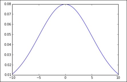
The most important continuous distribution is the standard normal distribution. You have, no doubt, either heard of the normal distribution or dealt with it. The idea behind it is quite simple. The PDF of this distribution is as follows:

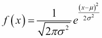
Here, μ is the mean of the variable and σ is the standard deviation. This might look confusing, but let's graph it in Python with a mean of 0 and a standard deviation of 1, as shown here:

import numpy as npimport matplotlib.pyplot as pltdef normal_pdf(x, mu = 0, sigma = 1):return (1./np.sqrt(2*3.14 * sigma**2)) * np.exp((-(x-mu)**2 / (2.* sigma**2)))x_values = np.linspace(-5,5,100)y_values = [normal_pdf(x) for x in x_values]
plt.plot(x_values, y_values)

We get this graph:

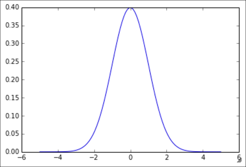
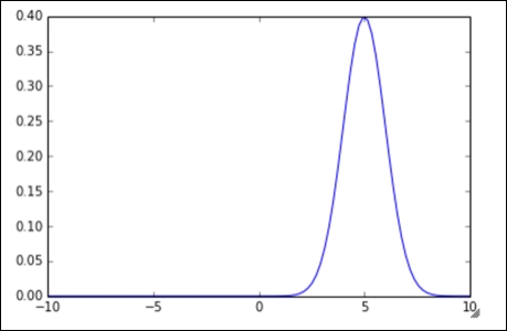
This gives rise to the all-too-familiar bell curve. Note that the graph is symmetrical around the x = 0 line. Let's try changing some of the parameters. First, let's try with :

Next, let's try with the value :

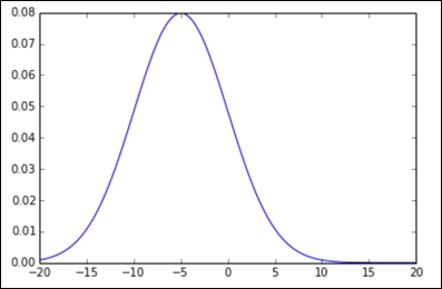
Lastly, we will try with the values :

In all the graphs, we have the standard bell shape that we are all familiar with, but as we change our parameters, we see that the bell might get skinnier, thicker, or move from left to right.

In the following chapters, which focus on statistics, we will make much more use of the normal distribution as it applies to statistical thinking.