
In the previous two chapters, you saw how to hone your dataset so that you defined only the rows and columns of data that you really need. Then you learned how to cleanse and complete the data that they contain. In this chapter, you will learn how to build on these foundations to deliver data that is ready to be molded into a structured and useable data model.
The generic term for this kind of data preparation in Power BI Desktop is
data mashup
. It covers the following:
- Joining datasets (or queries, if you prefer): This involves taking two queries and linking them so that you display the data from both sources as a single dataset. You will learn how to extend a query with multiple columns from a second query as well as how to aggregate the data from a second query and add this to the initial dataset. You will also see how to create complex joins when merging queries.
- Assembling data from the files in a folder: Here you will build on the knowledge acquired previously to use the Query Editor to filter the file types from a source folder and only amalgamate the ones that you choose.
- Pivoting and unpivoting data: If you need to switch data in rows to display as columns—or vice versa—then you can get the Power BI Desktop Query Editor to help you do exactly this. This means that you can guarantee that the data in all the tables that you are using conforms to a standardized tabular structure.
- Parsing column contents: This can be required to break down the contents of a column into data structured as a data table.
I want to be clear that separating data preparation into these two apparently contradictory approaches—reducing datasets only to augment them later—is not necessarily the way that you will work in practice. Given the range of features available in Power BI Desktop Query, I have simply tried to apply some structure to the way that they are explained. Hopefully, this will make the data-handling toolkit that is the Power BI Desktop Query Editor a little easier to understand. I imagine that when you are delving into data with Power BI Desktop, you will mix and alternate many of the techniques that are outlined in Chapters 6 through 8 in any order. After all, one of the great strengths of Power BI Desktop Query is that it does not impose any strict way of working and lets you experiment freely. So remember that you are at liberty to take any approach you want when transforming source data. The only thing that matters is that it gives you the result that you want.
The Power BI Desktop Query Editor View Ribbon
Until now, we have concentrated our attention on the Power BI Desktop Query Editor Home, Transform, and Add Column ribbons. This is for the good and simple reason that these ribbons are where nearly all the action takes place. There is, however, a fourth essential Power BI Desktop Query Editor ribbon—the View ribbon. The buttons that it contains are shown in Figure 8-1 and the options are explained in Table 8-1.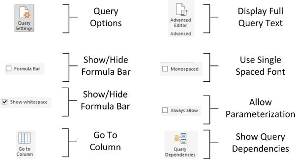
Figure 8-1.
The Power BI Desktop View ribbon
Table 8-1.
Power BI Desktop View Ribbon Options
Option
|
Description
|
|---|---|
Query Settings | Displays or hides the Query Settings pane at the right of the Power BI Desktop window. This includes the Applied Steps list. |
Formula Bar | Shows or hides the formula bar containing the M language code for a transformation step. |
Monospaced | Displays data in a monospaced (Courier) font. |
Show Whitespace | Shows whitespace and newline characters. |
Go to Column | Allows you to move to a column selected from those available. |
Always Allow | Allows parameterization. |
Advanced Editor | Displays the Advanced Editor dialog containing all the code for the steps in the query. |
Query Dependencies | Displays the sequence of query links and dependencies. |
Possibly the only option that is not immediately self-explanatory is the Advanced Editor button. It displays the code for all the transformations in the query as a single block of “M” language script.
Tip
Personally, I find that the Query Settings pane and the formula bar are too vital to be removed from the Power BI Desktop Query window when transforming data. Consequently, I tend to leave them visible. If you need the screen real estate, however, then you can always hide them for a while.
Merging Data
Until now, we have treated each individual query as if it existed in isolation. The reality, of course, is that you will frequently be required to use the output
of one query in conjunction with the output of another to join data from different tables in various ways. Assuming that the results of one query share a common field (or fields) with another query, you can “join” queries into a single data table. Power BI Desktop calls this a merge operation, and it enables you, among other things, to
- Look up data elements in another “reference” table to add lookup data. For example, you may want to add a client name where only the client code exists in your main table.
- Aggregate data from a “detail” table (such as invoice lines) and include the totals in a higher-grained table, such as a table of invoices.
Here, again, the process is not difficult. The only fundamental factor is that the two tables, or queries, that you are merging must have a shared field or fields that enable the two tables to match records coherently. Let’s look at a couple of examples.
Adding Data
First, let’s try looking up extra data that we will add to a query:
- 1.In a new, empty Power BI Desktop file, load both the worksheets in the C:PowerBiDesktopSamplesCH08SalesData.xlsx Excel file.
- 2.Click the Edit Queries button in the Home ribbon.
- 3.Click the query named Sales in the Queries pane of the Power BI Desktop Query window.
- 4.Click the Merge Queries button in the Home ribbon. The Merge dialog will appear.
- 5.In the upper part of the dialog —where an overview of the output from the current query is displayed—scroll to the right and click the ClientName column title. This column is highlighted.
- 6.In the popup under the upper table, select the Clients query. The output from this query will appear in the lower part of the dialog.
- 7.In the lower table, select the column title for the column—the join column—that maps to the column that you selected in step 4. This will also be the ClientName column. This column is then selected in the lower table. You may be asked to set privacy levels for the data sources. If this is the case, set them to Public.
- 8.Select Inner (only matching rows) from the Join Kind popup menu. The dialog will look like Figure 8-2.
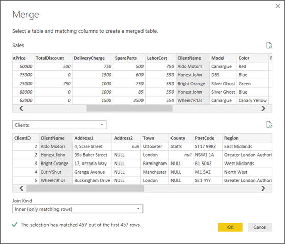 Figure 8-2.The Merge dialog
 - 9.Click OK. A new column is added to the right of the existing data table.
- 10.Scroll to the right of the existing data table and click the Expand icon to the right of the column name (it has probably been named New Column and every row contains the word Table). The popup list of all the available fields in this data table (or query, if you prefer) is displayed, as shown in Figure 8-3.
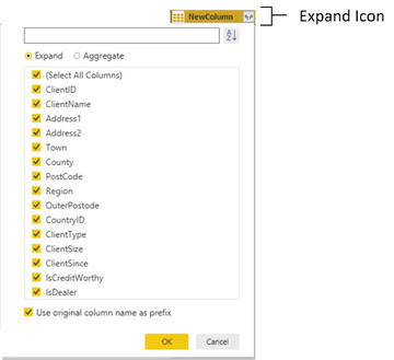 Figure 8-3.The fields available in a joined query
 - 11.Ensure that the Expand radio button is selected.
- 12.Clear the selection of all the columns by unchecking the (Select All Columns) check box.
- 13.Select the following columns:
- a.ClientName
- b.ClientSize
- c.ClientSince
- a.
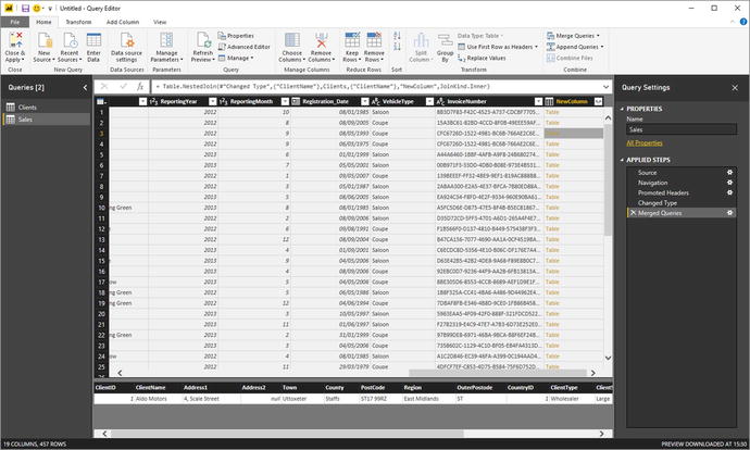
- 14.Click OK. The selected columns from the linked table are merged into the main table, and the link to the reference table (New Column) is removed.
- 15.Rename the columns that have been added, and apply and close the query.
You now have a single table of data that contains data from two linked data sources. Reprocessing the Sales query will also reprocess the dependent clients query and result in the latest version of the data being reloaded. Moreover, each of the columns that has been added has the title “NewColumn”, followed by the column name from the merged data source.
Note
You probably noticed that the Merge dialog indicated how many matching records there were in the two queries. This can be a useful indication that you have selected the correct column(s) to join the two queries.
Aggregating Data During a Merge Operation
If you are not just looking up reference data but need to aggregate data from a separate table and then add the results to the current query, then the process is largely similar. This second approach, however, is designed to suit another completely different requirement. Previously, you saw the case where the current query had many records that mapped to a single record in the lookup table. This second approach is for when your current (or main) query has a single record where there are multiple linked records in the second query. Consequently, you need to aggregate the data in the second table to bring the data across into the first table. Here is a simple example, using some of the sample data from the C:PowerBiDesktopSamples folder:
- 1.Find the InvoicesAndInvoiceLines.xlsx Excel source file in the C:PowerBiDesktopSamplesCH08 folder. Edit the two worksheets it contains (Invoices and InvoiceLines) into the Power BI Desktop Query Editor. This will create two queries.
- 2.Click the query named Invoices in the Queries pane on the left.
- 3.In the Home ribbon, click the Merge Queries button. The Merge dialog will open. You will see some of the data from the Invoices dataset in the upper part of the dialog.
- 4.Click anywhere inside the InvoiceID column. This column is selected.
- 5.In the popup, select the InvoiceLines query. You will see some of the data from the Invoices dataset in the lower part of the dialog.
- 6.Click anywhere inside the InvoiceID column for the lower table. This column is selected.
- 7.Select Inner (only matching rows) from the Join Kind popup menu. The dialog will look like Figure 8-4.
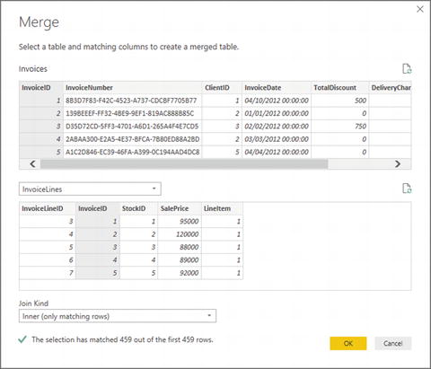 Figure 8-4.The Merge dialog when aggregating data
 - 8.Click OK.
- 9.Scroll to the right of the existing data table. You will see a new column (named NewColumn) that contains the word Table in every cell. This column will look something like Figure 8-5.
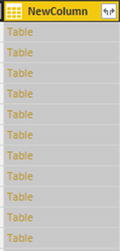 Figure 8-5.A merged column
 - 10.Click the Expand icon to the right of the new column title (the two arrows facing left and right). The popup list of all the available fields in the InvoiceLines query is displayed.
- 11.Select the Aggregate radio button.
- 12.Select the Sum Of SalePrice field.
- 13.Uncheck the “Use original column name as prefix” check box. The dialog will look like Figure 8-6.
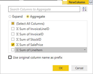 Figure 8-6.The available fields from a merged dataset
 - 14.Click OK.
Power BI Desktop will add up the total sale price for each invoice and add this as a new column. Naturally, you can choose the type of aggregation that you wish to apply (before clicking OK), if the sum is not what you want. To do this, place the cursor over the column that you want to aggregate
(see step 11 in the preceding exercise) and click the popup menu at the right of the field name. Power BI Desktop will suggest a set of options. The available aggregation options are explained in Table 8-2.
Tip
If you loaded the data instead of editing the query in step 1, simply Click the Edit Queries button in the Home ribbon to switch to the Query Editor.
Table 8-2.
Merge Aggregation Options
Option
|
Description
|
|---|---|
Sum | Returns the total value of the field. |
Average | Returns the average value of the field. |
Median | Returns the median value of the field. |
Minimum | Returns the minimum value of the field. |
Maximum | Returns the maximum value of the field. |
Count (All) | Counts all records in the dataset. |
Count (Not Blank) | Counts all records in the dataset that are not empty. |
The merge process that you have just seen, while not complex in itself, suddenly opens up many new horizons. It means that you can now create multiple separate queries that you can then use together to expand your data in ways that allow you to prepare quite complex datasets.
Here are a couple of comments I need to make about the merge operation:
- Only queries that have been previously created in the Power BI Desktop Query window can be used when merging datasets. So remember to connect to all the datasets that you require before attempting a merge operation.
- Refreshing a query will cause any other queries that are merged into this query to be refreshed also. This way you will always get the most up-to-date data from all the queries in the process.
Tip
You do not have to load a dataset to merge it with another query. You can simply edit it. This will establish a connection to the source data.
Types of Join
When merging queries
—either to join data or to aggregate values—you are faced with a choice when it comes to how to link the two queries. The choice of join can have a profound effect on the resulting dataset. Consequently, it is important to understand the six join types that are available. These are described in Table 8-3.
Table 8-3.
Join Types
Join Type
|
Explanation
|
|---|---|
Left Outer | Keeps all records in the upper dataset in the Merge dialog (the dataset that was active when you began the merge operation). Any matching rows (those that share common values in the join columns) from the second dataset are kept. All other rows from the second dataset are discarded. |
Right Outer | Keeps all records in the lower dataset in the Merge dialog (the dataset that was not active when you began the merge operation). Any matching rows (those that share common values in the join columns) from the upper dataset are kept. All other rows from the upper dataset (the dataset that was active when you began the merge operation) are discarded. |
Full Outer | All rows from both queries are retained in the resulting dataset. Any records that do not share common values in the join field(s) contain blanks in certain columns. |
Inner | Only joins queries where there is an exact match on the column(s) that are selected for the join. Any rows from either query that do not share common values in the join column(s) are discarded. |
Left Anti | Keeps only rows from the upper (first) query. |
Right Anti | Keeps only rows from the lower (second) query
. |
Note
When you use any of the outer joins, you are keeping records that do not have any corresponding records in the second query. Consequently, the resulting dataset contains empty values for some of the columns.
When you are expanding the column that is the link to a merged dataset, you have a couple of useful options that are worth knowing about:
- Use original column name as prefix
- Search columns to expand
Use the Original Column Name As the Prefix
You will probably find that some columns from joined queries can have the same names in both source datasets
. It follows that you need to identify which column came from which dataset. If you leave the check box selected for the “Use original column name as prefix” merge option (which is the default), any merged columns will include the source query name to help you identify the data more accurately.
If you find that these longer column names only get in the way, you can unselect this check box. This will leave the added columns from the second query with their original names. However, because Power BI Desktop cannot accept duplicate column names, any new columns will have .1, .2, and so forth, added to the column name.
Search Columns to Expand
If you are merging a query with a second query that contains a large number of columns, then it can be laborious to search for the columns that you want to include. To narrow your search you can enter a few characters from the column that you are looking for. The more characters you type, the fewer matching columns are displayed in the Expansion popup dialog
.
Joining on Multiple Columns
In the examples so far, you only joined queries on a single column. While this may be possible if you are looking at data that comes from a clearly structured source
(such as a relational database), you may need to extend the principle when joining queries from diverse sources. Fortunately, Power BI Desktop allows you to join queries on multiple columns when the need arises.
As an example of this, the sample data contains a file that I have prepared as an example of how to join queries on more than one column. This sample file contains data from the sources that you saw in previous chapters. However, they have been modeled as a data warehouse star schema. To complete the model, you need to join a dimension named Geography to a fact table named Sales so that you can add the field GeographySK to the fact table. However, the Sales table and the Geography table share three fields (Country, Region, and Town) that must correspond for the queries to be joined. The following explains how to perform a join using multiple fields:
- 1.Click Get Data, select Excel as the source, and in the C:PowerBiDesktopSamplesCH08StarSchema.xlsx Excel file select the two worksheets.
- 2.Click Edit Queries to open the Query Editor.
- 3.Select the Sales query from the list of existing queries from the Queries pane on the left of the Power BI Desktop Query window.
- 4.In the Home ribbon, click the Merge Queries button. The Merge dialog will appear.
- 5.In the popup list of queries, select Geography as the second query to join to the first (upper) query.
- 6.Select Inner (only matching rows) from the Join Kind popup.
- 7.In the upper list of fields (taken from the Sales table), Ctrl-click the fields CountryName and Region, in this order. A small number will appear to the right of each column header indicating the order that you selected the columns.
- 8.In the lower list of fields (taken from the Sales table) Ctrl-click in the fields CountryName and Region, in this order. A small number will appear to the right of each column header indicating the order that you selected the columns.
- 9.Verify that you have a reasonable number of matching rows in the information message at the bottom of the dialog. The dialog will look like Figure 8-7.
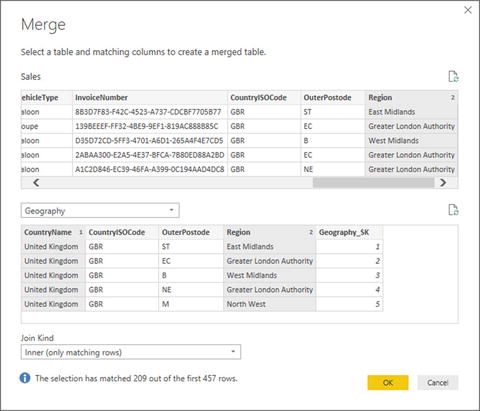 Figure 8-7.Joining queries using multiple columns
 - 10.Click OK.
You can then continue with the data mashup. In this example, that would be adding the GeographySK field to the Sales query and then removing the Country, Region, and Town fields from the Sales query.
There is no real limit to the number of columns that can be used when joining queries. It will depend entirely on the shape of the source data. However, each column used to define the join must exist in both datasets
and each pair of columns must be of the same (or a similar) data type.
Preparing Datasets for Joins
You could have to carry out a little preparatory work on real-world datasets before joining queries. More specifically, any columns that you join have to be the same basic data type. Put simply, you need to join text-based columns to other text-based columns, number columns to number columns, and date columns to date columns. If the columns are not the same data type, you receive a warning message when you try to join the columns in the Merge dialog.
Consequently, it is nearly always a good idea to take a look at the columns that you will use to join queries before you start the merge operation itself. Remember that data types do not have to be identical, just similar. So a decimal number type can map to a whole number, for instance.
You might also have to cleanse the data in the columns that are used for joins before attempting to merge queries. This could involve the following:
- Removing trailing or leading spaces in text-based columns
- Isolating part of a column (either in the original column or as a new column) to use in a join
- Verifying that appropriate data types are used in join columns
Correct and Incorrect Joins
Merging queries
is the one data mashup operation that is often easier in theory than in practice, unfortunately. If the source queries were based on tables in a relational or even dimensional database, then joining them could be relatively easy, as a data architect will (hopefully) have designed the database tables to allow for them to be joined. However, if you are joining two completely independent queries, then you could face several major issues:
- The columns do not map.
- The columns map, but the result is a massive table with duplicate records.
Let’s take a look at these possible problems.
The Columns Do Not Map
If the columns do not map (that is, you have joined the data but get no resulting records), then you need to take a close look at the data in the columns that you are using to establish the join. The questions you need to ask are as follows:
- Are the values in the two queries the same data type?
- Do the values really map—or are they different?
- Are you using the correct columns?
- Are you using too many columns and so specifying data that is not in both queries?
The Columns Map, but the Result Is a Massive Table with Duplicate Records
Joining queries depends on isolating unique data
in both source queries. Sometimes a single column does not contain enough information to establish a unique reference that can uniquely identify a row in the query.
In these cases, you need to use two or more columns to join queries—or else rows will be duplicated in the result. Therefore, once again, you need to look carefully at the data and decide on the minimum number of columns that you can use to join queries correctly.
Examining Joined Data
Joining data tables
is not always easy. Neither is deciding if the outcome of a merge operation will produce the result that you expect. So Power BI Desktop Query includes a solution to these kinds of dilemma. It can help you more clearly see what a join has done. More specifically, it can show you for each record in the first query exactly which rows are joined from the second query.
Do the following to see this in action:
- 1.Carry out steps 1 through 8 in the first example in the “Merging Data” section (in the “Adding Data” subsection).
- 2.Scroll to the right in the data table. You will see the new column named NewColumn (as shown in Figure 8-8).
- 3.Click to the right of the word Table in the row where you want to see the joined data. Note that you must not click the word Table. A second table will appear under the main query’s data table containing the data from the second query that is joined for this particular row. Figure 8-8 shows an example of this.
Figure 8-8.
Joined data
This technique is as simple as it is useful. There are nonetheless a few comments that I need to make:
- You can resize the lower table (and consequently display more or less data from the second joined table ) by dragging the bottom border of the top data table up or down.
- Clicking to the right of the word Table in the NewColumn column will enable the Expand and Aggregate buttons in the Transform ribbon.
- Clicking the word Table in the NewColumn column adds a new step to the query that replaces the source data with the linked data. You can also do this by right-clicking inside the NewColumn column and selecting Drill Down.
Note
Drilling down into the merged table in effect limits the query to the row(s) of the subtable. Consequently, you have to delete this step if you want to access all the data in the merged tables.
The Expand and Aggregate Buttons
Power BI Desktop Query
offers an alternative to using the NewColumn popup menu to expand or aggregate data when merging queries. If you have clicked to the right of the word Table in the NewColumn, you can then click the newly activated Expand button or Aggregate button in the Transform ribbon to display the Expand dialog or Aggregate dialog.
The only real difference between the dialogs and the popups is that the Expand dialog also has an option where you can add a new column prefix that you choose for the additional columns from the second query. You can see this in Figure 8-9.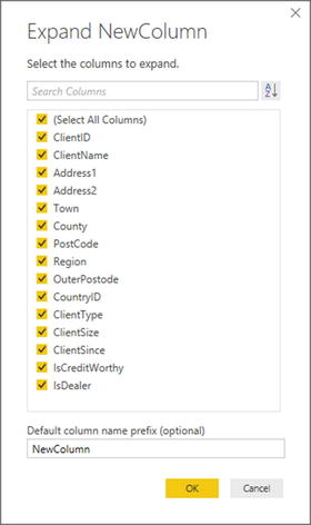
Figure 8-9.
The Expand New Column dialog
Appending Data
Not all source data is delivered in its entirety in a single file or as a single database table. You may be given access to two or more tables or files that have to be loaded into a single table in Excel or Power Pivot. In some cases, you might find yourself faced with hundreds of files—all text, CSV, or Excel format—and the requirement to load them all into a single table that you will use as a basis for your analysis. Well, Power BI Desktop can handle these eventualities, too.
Adding the Contents of One Query to Another
In the simplest case, you could have two data sources that are structurally identical (that is, they have the same columns in the same order), and all that you have to do is add one to another to end up with a query that outputs the amalgamated content of the two sources. This is called appending data, and it is easy, provided that the two data sources have identical structures; this means
- They have the same number of columns.
- The columns are in the same order.
- The data types are identical for each column.
- The columns have the same names.
As long as all these conditions are met, you can append the output of queries (which Power BI Desktop also calls Tables and many people, including me, refer to as datasets
) one into another. The queries do not have to have data that comes from identical source types, so you can append the output from a CSV file to data that comes from an Oracle database, for instance. As an example, we will take two text files and use them to create one single output:
- 1.Create queries to load each of the following text files into Power BI Desktop—without the final load step, which would output them to Excel or the Excel data model. Both files are in the C:PowerBiDesktopSamplesCH08MultipleIdenticalFiles folder:
- a.Colors_01.txt
- b.Colors_02.txt
- a.
- 2.Name the queries Colors_01 and Colors_02.
- 3.Open one of the queries (I use Colors_01, but either will do).
- 4.Click the Append Queries button in the Power BI Desktop Query Editor Home ribbon. The Append dialog will appear.
- 5.From the Select Table To Append popup, choose the query Colors_02.
- 6.Click OK.
The data from the two output
tables is placed in the current query. You can now continue with any modifications that you need to apply. You will notice that the column names are not repeated as part of the data when the tables are appended one to the other.
Adding Multiple Files from a Source Folder
Now let’s consider another possibility. You have been sent a load of files, possibly downloaded from an FTP site or received by e-mail, and you have placed them all into a specific directory. However, you do not want to have to carry out the process that you just saw and load files one by one if there are several hundred files. Another use for this approach is when you have to load files stored in multiple separate subdirectories. So here is a way to get Power BI Desktop to do the work of trawling through the directory and only loading files that correspond to a file name specification you have indicated. This approach extends the technique that you saw in Chapter 2, where you learned to load all the files in a directory.
- 1.Create a new Power BI Desktop file.
- 2.In the Power BI Desktop Home ribbon, click Get Data ➤ File in the Get Data dialog. Then select Folder to the right of the dialog.
- 3.Click Connect. The Folder dialog is displayed.
- 4.Click the Browse button and navigate to the folder that contains the files to load. In this example, it is C:PowerBiDesktopSamplesCH08. You can also paste in, or enter, the folder path if you prefer. The Folder dialog will look like Figure 8-10.
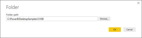 Figure 8-10.The Folder dialog
 - 5.Click OK. The Power BI Desktop window opens. The contents of the folder and all subfolders are listed as a table, as shown in Figure 8-11.
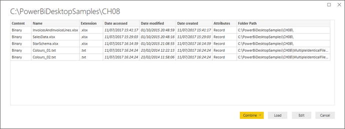 Figure 8-11.The folder contents in Power BI Desktop
 - 6.Click Edit. The Power BI Desktop Query Editor will display the list of files. This is shown in Figure 8-12.
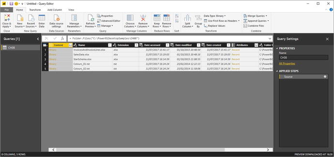 Figure 8-12.Files listed in the Power BI Desktop Query Editor
 - 7.As you want to load only text files, and avoid files of any other type, click the filter popup menu for the column title Extension and uncheck all elements except .txt. This is shown in Figure 8-13.
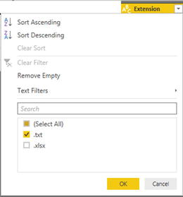 Figure 8-13.Filtering file types when loading multiple identical files
 - 8.Click OK. You will now only see the text files in the Query Editor.
- 9.Click the Expand icon (two downward-facing arrows) to the right of the first column title; this column is called Content and every row in the column contains the word Binary. Power BI will display the Combine Files dialog that you saw previously in Chapter 2.
- 10.Click OK. Power BI Desktop Query Editor will load all the files and display the result, as shown in Figure 8-14.
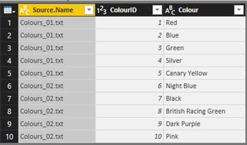 Figure 8-14.All files loaded from a folder
The contents of all the source files are now loaded into the Power BI Desktop Query Editor and can be transformed and used like any other dataset. This might involve removing superfluous header rows (as described in the next section). What is more, if ever you add more files to the source directory, and then click Refresh in the Home ribbon, all the source files are reloaded, including any new files added to the directory.
Note
You can also filter on directories, dates, or any of the file information that is displayed. Simply apply the filtering techniques that you learned in Chapter 6.
Removing Header Rows After Multiple File Loads
If the source files contained header rows, here is a practical way to remove them—fast—from the data:
- 1.If (but only if) each file contains header rows, then scroll down through the resulting table until you find a title element. In this example, it is the word ColourID in the ColourID column.
- 2.Right-click ColourID and select Text Filters ➤ Does Not Equal. All rows containing superfluous column titles are removed.
Note
If your source directory only contains the files that you want to load, then step 4 is unnecessary. Nonetheless, I always add steps like this in case files of the “wrong” type are added later, which would cause any subsequent process runs to fail. Equally, you can set filters on the file name to restrict the files that are loaded.
Changing the Data Structure
Sometimes your requirements go beyond the techniques that we have seen so far when discussing data cleansing and transformation. Some data structures need more radical reworking, given the shape of the data that you have acquired. I include in this category the following:
- Unpivoting data
- Pivoting data
- Transforming rows and columns
Each of these techniques is designed to meet a specific, yet frequent, need in data loading, and all are described in the next few pages.
Unpivoting Tables
From time to time, you may need to analyze data that has been delivered in a “pivoted” or “denormalized” format. Essentially, this means that information that really should be in a single column has been broken down and placed across several columns. An example of the first few rows of a pivoted dataset is given in Figure 8-15 and can be found in the C:PowerBiDesktopSamplesCH08PivotedDataSet.xlsx sample file.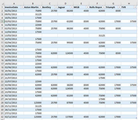
Figure 8-15.
A pivoted dataset
To analyze this data correctly, we really need the makes of the cars to be switched from being column titles to becoming the contents of a specific column. Fortunately, this is not hard at all:
- 1.In a new Power BI Desktop file, load the table PivotedCosts from the C:PowerBiDesktopSamplesCH08PivotedDataSet.xlsx file into Power BI Desktop. Ensure that the first row is set to be the table headers.
- 2.Switch to the Query Editor (unless it is already open) and select all the columns that you want to unpivot. In this example, this means all columns except the first one.
- 3.In the Transform ribbon, click the Unpivot Columns button (or right-click with the columns selected and choose Unpivot Columns from the context menu). The table is reorganized and the first few records look as they do in Figure 8-16. Unpivoted Columns is added to the Applied Steps list.
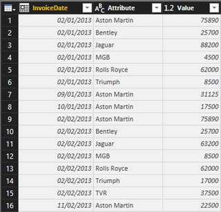 Figure 8-16.An unpivoted dataset
 - 4.Rename the columns that Power BI Desktop Query has named Attribute and Value.
The data is now presented in a standard tabular way, and so it can be used to create a data model and then produce reports and dashboards.
Unpivot Options
There are a couple of available options when you unpivot data using the Unpivot Columns button popup in the Transform ribbon:
- Unpivot Other Columns: This will add the contents of all the other columns to the unpivoted output.
- Unpivot Only Selected Columns: This will only add the contents of any preselected columns to the unpivoted output.
Pivoting Tables
On some occasions, you may have to switch data from columns to rows so that you can use it efficiently. This kind of operation is called pivoting data. It is—perhaps unsurprisingly—very similar to the unpivot process that you saw in the previous section.
- 1.Follow steps 1 through 3 of the previous section so that you end up with the table of data that you can see in Figure 8-16.
- 2.Click inside the column Attribute.
- 3.In the Transform ribbon, click the Pivot Column button. The Pivot Column dialog will appear.
- 4.Select Value (the column of figures) as the values column that is aggregated by the pivot transformation. The Pivot Column dialog will look like Figure 8-17.
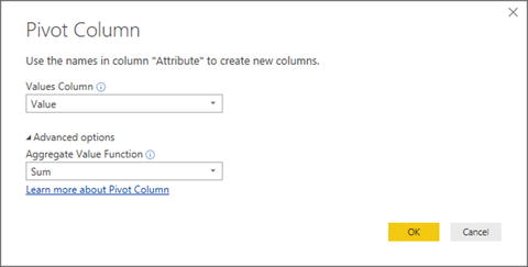 Figure 8-17.The Pivot Column dialog
 - 5.Click OK. The table is pivoted and looks like Figure 8-18. Pivoted Column is added to the Applied Steps list.
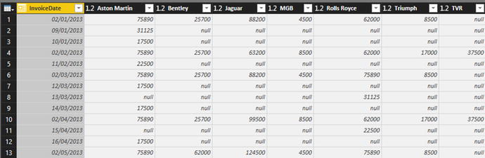 Figure 8-18.Pivoted data
Note
The Advanced Options section of the Pivot Column dialog lets you choose the aggregation operation that is applied to the values in the pivoted table.
The Unpivot button contains another menu option that is displayed if you click the small triangle to the right of the Unpivot button. This is the Unpivot Other Columns option that will switch the contents of columns into rows for all the columns that are not selected when you run the transformation.
Transposing Rows and Columns
On some occasions, you may have a source table where the columns need to become rows and the rows columns. Fortunately, this is a one-click transformation for Power BI Desktop. Here is how to do it:
- 1.Edit the C:PowerBiDesktopSamplesCH08DataToTranspose.xlsx Excel file in the Power BI Desktop Query Editor. You will need to select Sheet1. You will see a data table like the one in Figure 8-19.
 Figure 8-19.A dataset needing to be transposed
 - 2.In the Transform ribbon, click the Transpose button. The data is transposed and appears as two columns, just like the CountryList.txt file that you saw in Chapter 2.
- 3.Rename the columns.
Parsing JSON Files
In Chapter 2 you saw how to import JSON files. Previously, however, you only saw how to load the data into Power BI Desktop, and the file contents remained pretty much unusable. So now is the time to explain how you can use the Power BI Desktop Query Editor to convert the contents of a JSON file to a state that you can use in your data mashup.
- 1.In the Home ribbon, click Get Data ➤ File ➤ JSON, then click Connect.
- 2.Select the file C:PowerBiDesktopSamplesCH08Colors.json, and click Open. You will see a list of records like the one shown in Figure 8-20.
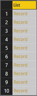 Figure 8-20.A JSON file after initial import
 - 3.You will see that the Query Editor has added the List Tools Transform ribbon. Click the To Table button in this ribbon. The To Table dialog will appear, as shown in Figure 8-21.
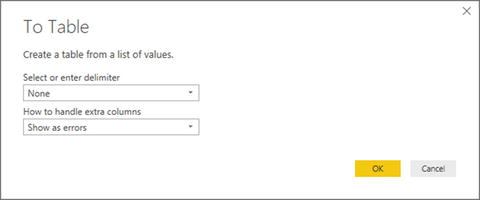 Figure 8-21.The To Table dialog
 - 4.Click OK. The list of data will be converted to a table. This means that it now shows the Expand icon at the right of the column title, as you can see in Figure 8-22.
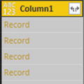 Figure 8-22.A JSON file converted to a table
 - 5.Click the Expand icon to the right of the column title, and in the popup dialog uncheck “Use original column name as prefix.”
- 6.Click OK. The contents of the JSON file now appear as a standard dataset, as you can see in Figure 8-23.
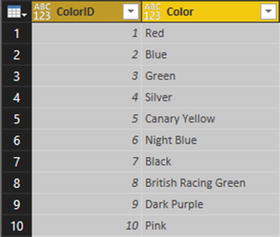 Figure 8-23.A JSON file transformed into a dataset
Although not particularly difficult, this process may seem a little counterintuitive. However, it certainly works, and you can use it to process complex JSON files so that you can use the data they contain in Power BI Desktop.
The List Tools Transform Ribbon
Power BI Desktop considers some data to be lists, not tables of data. It handles lists slightly differently, and displays a specific ribbon to modify list data. The List Tools Transform ribbon is explained in Figure 8-24 and Table 8-4.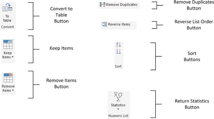
Figure 8-24.
The List Tools Transform ribbon
Table 8-4.
The List Tools Transform Ribbon Options
Option
|
Description
|
|---|---|
To Table | Converts the list to a table structure. |
Keep Items | Allows you to keep a number of items from the top or bottom of the list, or a range of items from the list. |
Remove Items | Allows you to remove a number of items from the top or bottom of the list, or a range of items from the list. |
Remove Duplicates | Removes any duplicates from the list. |
Reverse Items | Reverses the list order. |
Sort | Sorts the list lowest to highest or highest to lowest. |
Statistics | Returns calculated statistics about the elements in the list. |
Convert a Column to a List
Sometimes you will need to use data in a list format. Fortunately, Power BI Desktop lets you convert a column to a list really easily:
- 1.Open the Power BI Desktop file C:PowerBiDesktopSamplesCH08CH08Example1.pbix.
- 2.In the Home ribbon, click Edit Queries to open the Query Editor.
- 3.Select a column to convert to a list by clicking the column header. I will use the column Make in this example.
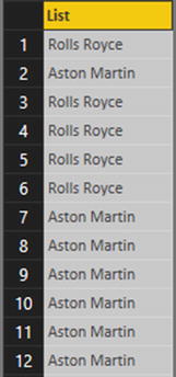
- 4.In the Transform ribbon, click Convert to List. The Query Editor will show the resulting list, as you can see in Figure 8-25.
Figure 8-25.
The list resulting from a conversion-to-list operation
Parsing XML Data from a Column
Some data sources, particularly database sources, include XML data actually inside a field. The problem here is that XML data is interpreted as plain text by Power BI Desktop when the data is loaded. If you look at Figure 8-26 you can see that this is not particularly useful.
So once again, Power BI Desktop has a solution to this kind of issue. To demonstrate how to convert this kind of text into usable data, you will find a sample Excel file (C:PowerBiDesktopSamplesCH08XMLInColumn.xlsx) that contains XML data as a column. Proceed as follows:
- 1.Edit the Excel file C:PowerBiDesktopSamplesCH08XMLInColumn.xlsx in the Query Editor. Select the only worksheet in this file: Sales.
- 2.Scroll to the right of the dataset and select the last column: AvailableColors. It looks like Figure 8-26.
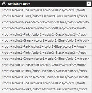 Figure 8-26.A column containing XML
 - 3.In the Add Column ribbon, click Parse ➤ XML . A new column will be added to the right. It will look like Figure 8-27, and will have the title XML .
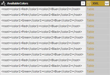 Figure 8-27.An XML column converted to a table column
 - 4.Click the Expand icon to the right of the XML column title and uncheck “Use original column name as prefix” in the popup dialog. Ensure that all the columns are selected and click OK. Two new columns (or, indeed, as many new columns as there are XML data elements) will appear at the right of the dataset. The Query Editor will look like Figure 8-28.
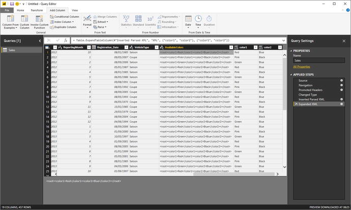 Figure 8-28.XML data expanded into new columns
 - 5.Delete the column containing the initial XML data.
Using this technique, you can now extract the XML
data that is embedded (or “nested” if you prefer) in source datasets
and use it to extend the original source data.
Parsing JSON Data from a Column
Sometimes you may encounter data containing JSON in a field, too. The technique to extract this data from the field inside the dataset and convert it to columns is virtually identical to the approach that you saw in the previous section for XML data.
Given that the approach is so similar, I will only provide a screenshot for the final result of the process. Here you will be able to see the source JSON as well as the columns of data that were extracted from the JSON and added to the dataset.
- 1.Edit the Excel file C:PowerBiDesktopSamplesCH08JSONInColumn.xlsx in the Query Editor. Select the only worksheet in this file: Sales.
- 2.Scroll to the right of the dataset and select the last column: AvailableColors.
- 3.In the Add Column ribbon, click Parse ➤ JSON. A new column will be added to the right and will have the title JSON.
- 4.Click the Expand icon to the right of the JSON column title and uncheck “Use original column name as prefix” in the popup dialog. Ensure that all the columns are selected and click OK. Two new columns (or, indeed, as many new columns as there are JSON data elements) will appear at the right of the dataset. The Query Editor will look like Figure 8-29.
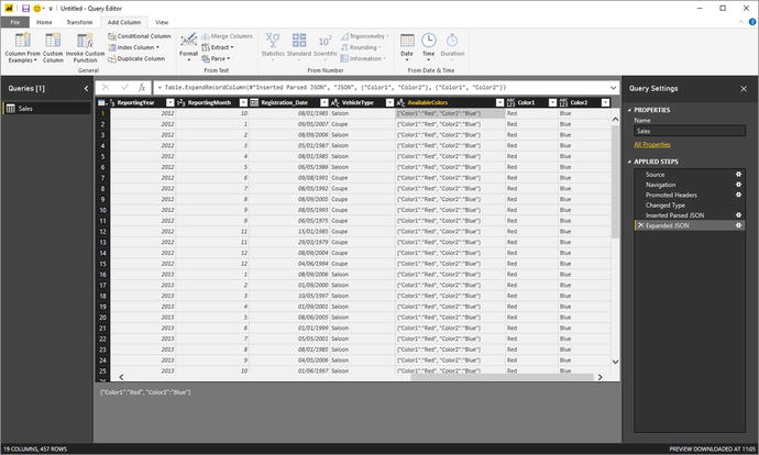 Figure 8-29.JSON data expanded into new columns
 - 5.Delete the column containing the initial JSON data.
Admittedly, the structure of the JSON data in this example is extremely simple. Real-world JSON
data could be much more complex. However, you now have a starting point upon which you can build when parsing JSON data that is stored in a column of a dataset.
Conclusion
This chapter showed you how to structure your source data into a valid data table from one or more potential sources. You saw how to pivot and unpivot data, to fill rows up and down with data, as well as how to create new columns of data from columns containing XML
or JSON
data.
Possibly the most important thing that you have learned is how to join individual queries so that you can add the data from one query into another. This can involve looking up data from a separate query or carrying the aggregated results from one query into another.
In this chapter and the six previous chapters, you have seen essentially a three-stage process: first, you find the data, then you load it into Power BI Desktop Query, and from there, you cleanse and modify it. The techniques that you can use are simple but powerful and can range from changing a data type to merging multiple data tables. Now that your data is prepared and ready for use, you can add it to the Power BI Desktop data model and start creating your Power BI Desktop dashboards.