
A considerable amount of data analysis—and probably most business intelligence—involves looking at how metrics evolve over time. You may need to aggregate sales by month, week, or year, for instance. Perhaps you want to compare figures for a previous month, quarter, or year with the figures for a current period. Whatever the exact requirement, handling time (by which we nearly always mean dates) is essential in Power BI Desktop.
Initially, using time functions in Power BI Desktop may only be limited to extracting time intervals from the available data and grouping results by units of time, such as days, weeks, months, quarters, and years. As you will find out in the first part of this chapter, DAX makes this kind of analysis really simple.
However, Power BI Desktop can also add what is called
time intelligence
to data models. This massively useful capability can take your analysis to a fundamentally higher level. This approach involves adding a separate table (called a date or time
dimension
) to the data model and then adding DAX functions that enable you to see how data evolves over time. Consequently, this chapter also includes an introduction to time intelligence using a wide range of DAX formulas that are available to help you create time-based calculations quickly and easily.
In this chapter, we continue to develop the file that you extended in the two previous chapters. Should you need it, a complete version of this file (CarSalesDataWithNewColumnsAndMeasures.pbix) is available on the Apress web site, including the extensions added in the previous chapter, in the folder C:PowerBiDesktopSamplesCH13.
Simple Date Calculations
Data analysis often involves looking at how key metrics evolve over time. Power BI Desktop can help you group and isolate date and time elements
in your data. Since dates (and time) are often a continuous stream of dates in a dataset, it can be useful to isolate the years, months, weeks, and days in a table alongside the date that a row contains so that you can create tables or visuals that group and aggregate records into these more comprehensible “buckets.” You can then display and compare data over years and months, for instance, in order to tease out the real insights that your raw data contains.
For the first example of how DAX can help you to categorize records using date-based criteria
, let’s imagine that you envisage creating a couple of charts. First, you need one that lets you track sales over the years that Brilliant British Cars has traded. Then you want a second graphic that looks at sales for each month over the years. Unfortunately (for the moment at least), your data model does not contain columns that show the year or the month of a sale, and Power BI Desktop does not let you create metrics as part of a visualization. You have to have the metric available in the data model if you plan to use it in a dashboard element
. Moreover, as you will see in Chapters 14 through 22, it is best if you have all the metrics in place before you create any visualizations. Indeed, this is precisely the reason that you are learning how to extend the data model with new columns using DAX. The following explains how to create these two new columns
in the Invoices table:
- 1.Open the Power BI Desktop file C:PowerBiDesktopSamplesCH13CarSalesDataWithNewColumnsAndMeasures.pbix.
- 2.Click the Data icon.
- 3.Select the Invoices table in the Fields list.
- 4.In the Modeling ribbon, click the New Column button.
- 5.In the formula bar to the left of the equals sign, replace Column with Sale Year.
- 6.Click to the right of the equals sign.
- 7.Enter (or start typing) and then select YEAR(.
- 8.Enter a left square bracket: [.
- 9.Select the InvoiceDate field.
- 10.Add a final right parenthesis to complete the YEAR() function.
- 11.Confirm the formula by pressing Enter or clicking the tick icon in the formula bar. The new column will display the year of each sale.
- 12.Repeat steps 2 through 9, only use the DAX formula MONTH() instead of YEAR(), and name the new column Sale Month.
The formula for the two new columns will be
Sale Month = MONTH([InvoiceDate])
Sale Year = YEAR([InvoiceDate])
Figure 13-1 shows what the Invoices table looks like with these two new columns added.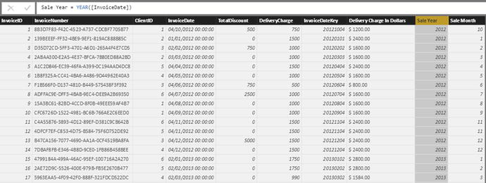
Figure 13-1.
The YEAR() and MONTH() DAX functions
In Chapters 15 through 20, you see how to use metrics like these to create visualizations that explore the way that sales have evolved over time.
Note
To extract part of a date like this, the column that you are using for the original data must be of the date data type or be capable of being interpreted as a date by Power BI Desktop.
This example illustrated two of the DAX date and time functions. Inevitably, there are many other functions that you can apply to extract a date or time element from a date field. Since they all follow the same principles as those that you have just seen (with the exception of the NOW() and TODAY() functions that are explained in a couple of pages’ time), it is easier to list them in Table 13-1 rather than provide a set of nearly identical examples.
Table 13-1.
DAX Date and Time Functions
Function
|
Description
|
Example
|
|---|---|---|
YEAR()
| Extracts the year element from a date. |
YEAR([InvoiceDate])
|
MONTH()
| Extracts the month number from a date. |
MONTH([InvoiceDate])
|
DAY()
| Extracts the day number from a date. |
DAY([InvoiceDate])
|
WEEKDAY()
| Extracts the weekday from a date. Sunday is 1, Monday is 2, and so forth. |
WEEKDAY([InvoiceDate])
|
WEEKNUM()
| Extracts the number of the week in the year from a date. |
WEEKNUM([InvoiceDate])
|
HOUR()
| Extracts the hour from a time or datetime column. |
HOUR([InvoiceDate])
|
MINUTE()
| Extracts the minutes from a time or datetime column. |
MINUTE([InvoiceDate])
|
SECOND()
| Extracts the seconds from a time or datetime column. |
SECOND([InvoiceDate])
|
EOMONTH()
| Returns the last day of the month from a date. |
EOMONTH([InvoiceDate])
|
NOW()
| Returns the current date and time. |
NOW()
|
TODAY()
| Returns the current date. |
TODAY()
|
DATE()
| Lets you enter a date as year, month, and day. |
DATE(2015, 07, 25)
|
TIME()
| Lets you enter a time as hours and minutes. |
TIME(19, 57)
|
DATEDIFF()
| Calculates the difference between two dates and/or times expressed as a number of specified periods. |
DATEDIFF([InvoiceDate], DATE(2025, 07, 25), YEAR)
|
STARTOFMONTH()
| Selects the first day of the month for a date. |
STARTOFMONTH(Invoices[SaleDate])
|
STARTOFQUARTER()
| Selects the first day of the quarter for a date. |
STARTOFQUARTER(Invoices[SaleDate])
|
STARTOFYEAR()
| Selects the first day of the year for a date. |
STARTOFYEAR(Invoices[SaleDate])
|
ENDOFMONTH()
| Selects the last day of the month for a date. |
ENDOFMONTH(Invoices[SaleDate])
|
ENDOFQUARTER()
| Selects the last day of the quarter for a date. |
ENDOFQUARTER(Invoices[SaleDate])
|
ENDOFYEAR()
| Selects the last day of the year for a date. |
ENDOFYEAR(Invoices[SaleDate])
|
YEARFRAC()
| Calculates the fraction of the year represented by the number of whole days between two dates. |
YEARFRAC(Stock[PurchaseDate],Invoices[SaleDate])
|
Note
If you define a field as having a date or datetime data type, then Power BI Desktop always creates a hierarchy of Year ➤ Quarter ➤ Month ➤ Day in the visual that you are creating. This can become annoying when all you need is the day. So it is well worth creating a well-structured date dimension table, as described later in this chapter, so that you only use the exact date element that you want, rather than have Power BI Desktop make assumptions for you.
Date and Time Formatting
When dealing with dates and times in Power BI Desktop, you may not need to go to the lengths of extracting a part of a date field, but may simply need to display a date in a different way. Rather like Excel, DAX can help you to do this quickly and easily using the
FORMAT() function
.
Suppose that you want to have the InvoiceDate field displayed in a specific date format for use in certain visualizations. The following explains how you can do this. The finished formula is in step 11 if you prefer to use this.
- 1.Select the Invoices table in the Fields list.
- 2.In the Modeling ribbon, click the New Column button.
- 3.In the formula bar to the left of the equals sign, replace Column with UKDate.
- 4.Click to the right of the equals sign.
- 5.Enter (or start typing and then select) FORMAT(.
- 6.Enter a left square bracket: [.
- 7.Select the InvoiceDate field.
- 8.Add a comma.
- 9.Enter the format code “D-MMM-YYYY” (include the double quotes).
- 10.Add a final right parenthesis to complete the FORMAT() function.
- 11.Replace the word Column with UKDate. The formula bar will display the following code:UKDate = FORMAT([InvoiceDate], "D-MMM-YYYY")
- 12.Confirm the formula by pressing Enter or clicking the tick icon in the formula bar. The new column will display the sale date in a different format.
If you look at Figure 13-2, you see what the newly formatted invoice data field looks like in the new column.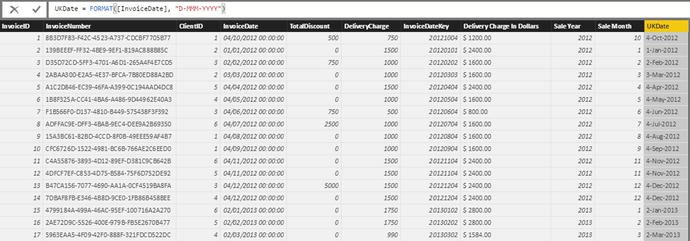
Figure 13-2.
Applying the FORMAT() function
Note
To reformat a date like this, the column that you are using for the original data must either be of the date data type or be capable of being interpreted as a date by Power BI Desktop.
The date format that you applied in this example was not predefined by DAX in any way. In fact, it was assembled from a set of day, month, and year codes that you can combine to create the date format that you want. Table 13-2 explains the codes that are available.
Table 13-2.
Custom Date Formats
Format Code
|
Description
|
Example
|
|---|---|---|
d
| The day of the month. |
"d MMM yyyy" produces 2 Jan 2016 |
dd
| The day of the month with a leading zero when necessary. |
"dd MMM yyyy" produces 02 Jan 2016 |
ddd
| The three-letter abbreviation for the day of the week. |
"ddd d MMM yyyy" produces Sat 2 Jan 2016 |
dddd
| The day of the week in full. |
"ddd dd MMM yyyy" produces Saturday 02 Jan 2016 |
M
| The number of the month
. |
"dd M yyyy" produces 02 1 2016 |
MM
| The number of the month with a leading zero when necessary. |
"dd MM yyyy" produces 02 01 2016 |
MMM
| The three-letter abbreviation for the month. |
"dd MMM yyyy" produces 02 Jan 2016 |
MMMM
| The full month. |
"dd MMMM yyyy" produces 02 January 2016 |
yy
| The year as two digits. |
"d MMM yy" produces 2 Jan 16 |
yyyy
| The full year. |
"MMMM yyyy" produces January 2016 |
If you do not want to build your own date formats, then you can choose from the seven predefined date and time formats that Power BI Desktop has available. These are explained in Table 13-3.
Table 13-3.
Predefined Date Formats
Format Code
|
Description
|
Example
|
Comments
|
|---|---|---|---|
Short Date | The short date as defined in the PC’s settings. |
FORMAT([InvoiceDate], "Short Date")
| Formats the date using figures only. |
Medium Date | The medium date as defined in the PC’s settings. |
FORMAT([InvoiceDate], "Medium Date")
| Formats the date with the month as a text and the day of the week. |
Long Date | The long date as defined in the PC’s settings. |
FORMAT([InvoiceDate], "Long Date")
| Formats the date with the month as a text and the day of the week. |
General Date | The date defined by the local PC’s culture settings. |
FORMAT([InvoiceDate], "General Date")
| Formats the date defined by the local PC’s culture settings. |
Long Time | The long time
as defined in the PC’s settings. |
FORMAT([InvoiceDate], "Long Time")
| Formats the datetime or time column with the hour and minutes of the day. |
Medium Time | The medium time as defined in the PC’s settings. |
FORMAT([InvoiceDate], "Short Time")
| Formats the datetime or time column with the hour and minutes of the day. |
Short Time | The short time as defined in the PC’s settings. |
FORMAT([
InvoiceDate
], "Short Time")
| Formats the datetime or time column with the hour and minutes and seconds of the day. |
Note
As I explained in Chapter 11, the FORMAT() function converts a field to a text, so you need to be aware that this has the potential to restrict its use if further calculations are applied to the result produced by this formula. In my opinion, it is essentially useful when applied to modify the way that dates are displayed.
Calculating the Age of Cars Sold
To continue with elementary DAX formulas—and as an admittedly extremely simple example—I will presume that we need to calculate the age of every car sold relative to the current date. As the source data contains the registration date for each vehicle, this will not be difficult. So, you have to create the formula that you can see finished in step 8:
- 1.With the Stock table selected, activate the Modeling ribbon and click the New Column button.
- 2.Enter a left parenthesis to the right of the equals sign.
- 3.Type NOW() . Make sure that you add the left and right parentheses even if these remain empty.
- 4.Enter a minus sign and then enter (or select) [Registration_Date].
- 5.Enter a right parenthesis. This corresponds to the left parenthesis before the NOW() function.
- 6.Enter a forward slash (the division symbol).
- 7.Enter 365.
- 8.Replace Column with VehicleAge. The formula should look like this:VehicleAge=(NOW()-[Registration_Date])/365
- 9.Press Enter or click the tick box in the formula bar. The formula will be added to the entire new column. Figure 13-3 shows you a small sample of the result of this operation.
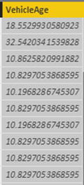 Figure 13-3.Calculated output using the NOW() function
Let me be clear, this is not the only way to calculate a time difference using DAX. It is probably not even the best one. It is merely a simple yet (I hope) comprehensible introduction to a DAX Date/Time calculation formula and it reminds you just how close a cousin DAX is to the Excel formula language. It also shows you an easy way to see exactly what DAX functions are available and what they do, since each function displays a brief explanation when you hover the mouse pointer over it.
Adding Time Intelligence to a Data Model
I want now to explain the vital set of functions that concern time, or rather, the dates used in analyzing data. Power BI Desktop calls this time intelligence (even though it nearly always refers to the use of date ranges). Applying this kind of temporal analysis can be a fundamental aspect of data presentation in business intelligence. After all, what enterprise does not need to know how this year’s figures compare to last year’s and what kind of progress is being made?
Time intelligence
always requires a valid date table, which is one of the reasons why we will now spend a certain amount of time creating this core pillar of a successful data model. Then the date table has to be joined to the table containing the data that you want to compare over time on a date field. The good news is that once you have a valid date table, and have acquainted yourself with a handful of data and time functions in DAX, you can deliver some extremely impressive results. These kinds of calculations can cover (among other things) the following:
- YearToDate, QuarterToDate, and MonthToDate calculations
- Comparisons with previous years, quarters, or months
- Rolling aggregations over a period of time, such as the sum for the last three months
- Comparison with a parallel period in time, such as the same month in the previous year
An introduction to time intelligence in Power BI Desktop gives you a taste of some of the DAX functions that you are likely to use when analyzing data over time. To begin with, you will learn how to create a date table. Then you will look at some of the different types of calculations that you can create to analyze data over time.
Creating and Applying a Date Table
For time intelligence to work, you need a table that contains an uninterrupted range of dates that begins at least at the earliest date in your data, and that ends with a date at least equal to the final date in your data. In practice, this will nearly always mean creating a date table that begins on the 1st of January of the earliest date in your data and that ends on the 31st of December of the last year for which you have data. Once you have your date table, you can join it to one of the tables in your data model and then begin to exploit all the time-related analytical functions
of Power BI Desktop.
The good news is that you can use Power BI Desktop itself to create a date table. It is also possible to import a contiguous range of dates from other applications such as Excel
. Because I prefer you to come to appreciate the breadth and depth of DAX, I will explain how to implement a date table directly in Power BI Desktop.
Creating the Date Table
The first requirement before starting to apply time intelligence is to have a valid date table. The following steps explain one way to create a date table using and extending your newly acquired DAX skills:
- 1.In Data View, activate the Modeling ribbon and click the New Table button. The expression Table = will appear in the formula bar.
- 2.Replace the word Table with DateDimension.
- 3.Click to the right of the equals sign and enter CALENDAR(.
- 4.Enter “1/1/2012” (include the double quotes). This is the starting date for a table of dates. I am assuming here that your computer is configured for the UK or European date format. If this is not the case, then enter the date as you would normally using your local date format.
- 5.Enter a comma.
- 6.Enter “31/12/2016” (or the equivalent date format that represents the 31st of December 2016 in your local date format). This is the end date for a table of dates.
- 7.Enter a right parenthesis. This corresponds to the left parenthesis of the CALENDAR() function. The formula bar will display this:DateDimension = CALENDAR( "1/1/2012", "31/12/2016" )
- 8.Press Enter or click the tick icon in the formula bar. Power BI Desktop will create a table containing a single column of dates from the 1st of January 2012 until the 31st of December 2016.
- 9.In the Fields list, right-click the Date field in the DateDimension table and select Rename. Rename the Date field to DateKey. The date table will look like Figure 13-4.
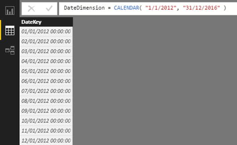 Figure 13-4.An initial date table for a time dimension
 - 10.
Table 13-4.
DAX Formulas to Extend a Date Table
Column Title
|
Formula
|
Comments
|
|---|---|---|
FullYear |
YEAR([DateKey])
| Isolates the year as a four-digit number. |
ShortYear |
VALUE(Right(Year([DateKey]),2))
| Isolates the year as a two-digit number. |
MonthNumber |
MONTH([DateKey])
| Isolates the number of the month in the year as one or two digits. |
MonthNumberFull |
FORMAT([DateKey], "MM")
| Isolates the number of the month in the year as two digits, with a leading zero for the first nine months. |
MonthFull |
FORMAT([DateKey], "MMMM")
| Displays the full name of the month. |
MonthAbbr |
FORMAT([DateKey], "MMM")
| Displays the name of the month as a three-letter abbreviation. |
WeekNumber |
WEEKNUM([DateKey])
| Shows the number of the week in the year. |
WeekNumberFull |
FORMAT(Weeknum([DateKey]), "00")
| Shows the number of the week in the year with a leading zero for the first nine weeks. |
DayOfMonth |
DAY([DateKey])
| Displays the number of the day of the month. |
DayOfMonthFull |
FORMAT(Day([DateKey]),"00")
| Displays the number of the day of the month with a leading zero for the first nine days. |
DayOfWeek |
WEEKDAY([DateKey])
| Displays the number of the day of the week. |
DayOfWeekFull |
FORMAT([DateKey],"dddd")
| Displays the name of the weekday. |
DayOfWeekAbbr |
FORMAT([DateKey],"ddd")
| Displays the name of the weekday as a three-letter abbreviation. |
ISODate |
[FullYear] & [MonthNumberFull] & [DayOfMonthFull]
| Displays the date in the ISO (internationally recognized) format of YYYYMMDD. |
FullDate
|
[DayOfMonth] & " " & [MonthFull] & " " & [FullYear]
| Displays the full date with spaces. |
QuarterFull |
"Quarter " & ROUNDDOWN(MONTH([DateKey])/4,0)+1
| Displays the current quarter. |
QuarterAbbr |
"Qtr " &ROUNDDOWN(MONTH([DateKey])/4,0)+1
| Displays the current quarter as a three-letter abbreviation plus the quarter number. |
Quarter |
"Q" &ROUNDDOWN(MONTH([DateKey])/4,0)+1
| Displays the current quarter in short form. |
QuarterNumber |
ROUNDDOWN(MONTH([DateKey])/4,0)+1
| Displays the number of the current quarter. This is essentially used as a Sort By column. |
QuarterAndYear |
DateDimension[Quarter] & " " & DateDimension[FullYear]
| Shows the quarter and the year. |
MonthAndYearAbbr |
DateDimension[MonthAbbr] & " " & [FullYear]
| Shows the abbreviated month and year. |
QuarterAndYearNumber |
[FullYear] & [QuarterNumber]
| Shows the year and quarter numbers. This is essentially used as a Sort By column. |
YearAndWeek |
VALUE([FullYear] &[WeekNumberFull])
| Indicates the year and week. The VALUE() function ensures that the figure is considered as numeric by Power BI Desktop. |
YearAndMonthNumber
|
VALUE(DateDimension[FullYear] & DateDimension[MonthNumberFull])
| A numeric value for the year and month. This is essentially used as a Sort By column. |
The first few columns of the DateDimension table should now look like Figure 13-5.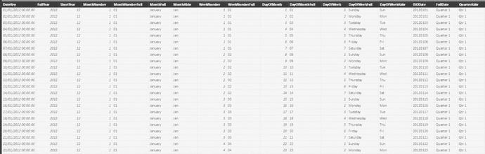
Figure 13-5.
The completed DateDimension table
The point behind creating all these ways of expressing dates and parts of dates is that you can now use them in your tables, charts, and gauges to aggregate and display data over time. Any record that has a date element can now be expressed visually; not just as the date itself, but shown as and aggregated as years, quarters, months, or weeks. The trick is to prepare all the time groupings that you are likely to need in the date table of your dashboards. However, you do not need to worry if you find yourself later needing an extra column or two further down the line, because you can always add columns that contain other date elements.
Adding Sort By Columns to the Date Table
In Chapter 11, you saw how to sort a column
using the data in another column to provide the sort order. This technique is essential when dealing with date tables, as you want to be sure that any visualizations that contain date elements appear in the right order. The classic example is months. As things stand, if you were to use the MonthFull column or MonthAbbr column in a chart or table, then you would see the month names appearing on an axis or in a column in alphabetical order.
To avoid this, you have to add one final tweak to the date table and apply a Sort By column to certain of the date elements in other columns. Since you saw how this is done in Chapter 11, now I will only provide the list of columns that need this extra tweak, rather than reiterating all the details. Table 13-5 gives you the required information to extend the data table so that all date elements are sorted correctly.
Table 13-5.
The Sort By Columns
Needed for the Date Table
Column
|
Sort By Column
|
|---|---|
FullDate | DateKey |
MonthFull | MonthNumber |
MonthAbbr | MonthNumber |
DayOfWeekFull | DayOfWeek |
DayOfWeekAbbr | DayOfWeek |
Quarter And Year | QuarterAndYearNumber |
MonthAndYearAbbr | YearAndMonthNumber |
MonthAndYear | YearAndMonthNumber |
Date Table Techniques
When using date tables to invoke time intelligence in DAX, there are two fundamental principles that must always be applied. I realize that I mention them elsewhere, but they are so essential that they bear repetition.
- The date range must be continuous; that is, there must not be any dates missing in the column that contains the list of calendar days in the table of dates.
- The date range must encompass all the dates that you are using in other tables in the data model.
The first requirement is covered by the use of the
CALENDAR() function
to create a date table. The second can require that you discover the lower and upper date thresholds in one or more tables of dates. Since this can be a little laborious (not to mention error-prone), it is probably easier to get DAX to find these dates for you and apply them to the CALENDAR() function.
Consequently, once you know where the lowest and highest dates are in your data model (even if they are in separate tables), you can use these dates as the lower and upper boundaries of the CALENDAR() function. In the case of the Brilliant British Cars data, the formula could read as follows:
DateDimension = CALENDAR(MIN('Stock'[PurchaseDate]), MAX('Invoices'[InvoiceDate]))
This formula shows that you can apply two functions
that you have seen already—MIN() and MAX()—with date and datetime data types. They simply tell DAX to find the earliest and latest dates in a column.
Alternatively, and as a nod to best practice, you may prefer to ensure that the date dimension always covers entire years of dates. In this case, the formula to create the table would be as follows:
DateDimension = CALENDAR(STARTOFYEAR(MIN('Stock'[PurchaseDate])), ENDOFYEAR(MAX('Invoices'[InvoiceDate])))
This formula extends the DAX calculation by using two functions that were explained in Table 13-1:
- STARTOFYEAR(): Deduces the first day of the year.
- ENDOFYEAR(): Deduces the last day of the year.
This formula also shows you that you can define a date range using different columns, or even different tables when you are specifying a date range. This is particularly useful when defining a date table.
Note
The principal advantage of looking up the date boundaries like this is that they update automatically as the source data changes. So if the Stock table or Invoices table is extended in the data source to contain further rows with dates outside the existing date range, then the DateDimension table will also grow to encompass these new dates.
Creating a data table can be fun, but nonetheless takes a few minutes. So here’s a tip that I can give you: create a Power BI Desktop file that contains nothing but a date dimension table (using a manually defined start date and end date, just as you saw at the beginning of this example) with all the other columns added. You can then make copies of this “template” file and use them as the basis for any new data models that you create. This can include replacing the fixed threshold dates with references to the data in tables, as mentioned previously.
Adding the Date Table to the Data Model
Now that you have a date table, you can integrate it with your data model so that you can start to apply some of the time intelligence that DAX makes possible.
- 1.Click the Relationships View icon to display the tables in the data model.
- 2.In the Home ribbon, click the Manage Relationships button. The Manage Relationships dialog will appear.
- 3.Click the New button. The Create Relationship dialog will appear.
- 4.At the top of the dialog, select the DateDimension table from the popup list.
- 5.Once the sample data from the DateDimension table is displayed, click inside the DateKey column to select it.
- 6.Under the DateDimension table sample data, select the Invoices table from the popup list.
- 7.Once the sample data from the Invoices table is displayed, click inside the InvoiceDate column to select it. The dialog will look like Figure 13-6.
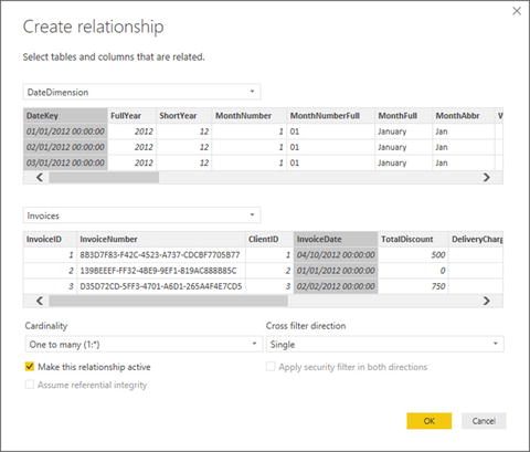 Figure 13-6.Adding a date dimension to the data model
 - 8.Click OK. The relationship will appear in the Manage Relationships dialog.
- 9.Click Close. The DateDimension table will appear in the data model joined to the Invoices table. You can see this in Figure 13-7.
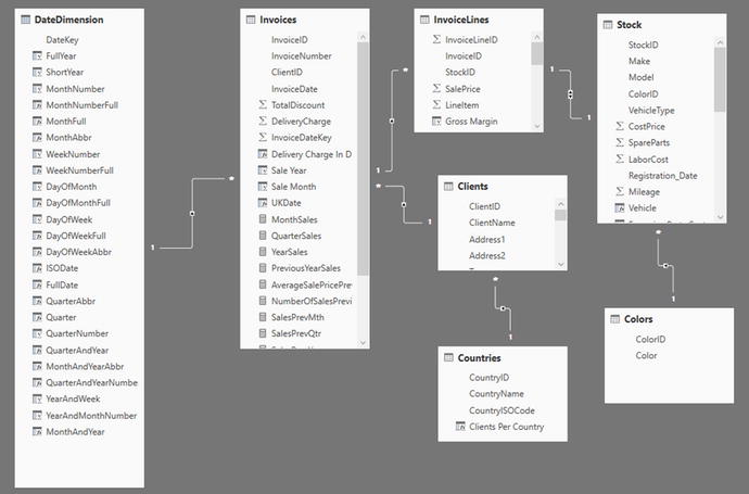 Figure 13-7.A data model with a data table added
Note
For time intelligence in Power BI Desktop
to work correctly, the fields used to join a date table and a data table must both be set to the date or datetime data type.
Calculating the Difference Between Two Dates
Now that you have a date dimension in the data model, you can create some more powerful date and time calculations. For instance, and as you would probably expect, DAX can do more than just specify a number of days. As befits a formula language that is designed to aid in business analysis, it can deduce the time between two dates expressed as the following:
- Years
- Months
- Weeks
- Days
- Hours
- Minutes
- Seconds
This can be extremely useful when you want to classify records according to a duration, and can be calculated using the DATEDIFF() function. The
DATEDIFF() function
expects you to apply three parameters when calculating an interval:
- The start date for the calculation of the interval.
- The end date up until when the interval will be calculated.
- The interval to calculate. This could be in years, days, or minutes, for example.
As an example, imagine that you want to display the number of weeks that each vehicle remained in stock, as this will help you to determine the fastest-selling models and consequently optimize the company’s cash flow. As the data contains both the purchase date for each vehicle and its sale date (even if the two are in different tables), this can be done using the DAX DATEDIFF() function (as you can see in the finished formula in step 12) as follows:
- 1.In the CarSalesDataWithNewColumnsAndMeasures.pbix file, click the Data View icon and then click the Stock table in the Fields list.
- 2.Click the New Column button in the Modeling ribbon. A new column named Column will appear at the right of any existing columns.
- 3.To the right of the equals sign, enter DATEDIFF(. You will see that as you enter the first few characters, the list of functions will list all available functions beginning with these characters. You can click the function name to have it appear in the formula bar.
- 4.Press the [ key. The list of available fields from the current table will appear.
- 5.Select the [PurchaseDate] field.
- 6.Enter a comma.
- 7.Type RELATED(. The popup will display all the fields that can be linked via the data model to this table.
- 8.Scroll down the list and select Invoices[InvoiceDate].
- 9.Add a right parenthesis to close the RELATED() function.
- 10.Enter a comma. A popup list of available intervals will appear.
- 11.Select WEEK.
- 12.Add a final right parenthesis. The formula will look like this:Weeks In Stock = DATEDIFF([PurchaseDate],RELATED(Invoices[InvoiceDate]),WEEK)
- 13.Press Enter or click the tick box in the formula bar. The formula will be added to the entire new column. You can now rename it Weeks In Stock . Figure 13-8 shows you a small sample of the result of this operation.
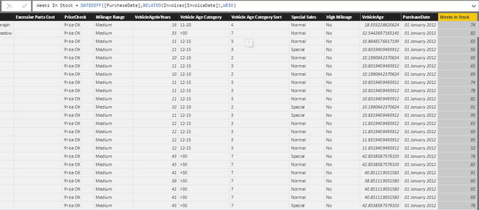 Figure 13-8.The results of a DATEDIFF() function
You can now see the number of weeks that each vehicle was in stock before being sold and use this figure in Power BI Desktop dashboards. Only complete intervals are displayed. In other words, if you have selected YEAR as the interval, then the difference between the two dates must be fractionally more than one year for the function to return 1. Notice that you used the
RELATED() function
again to compare elements from separate tables. Once again, Power BI Desktop only listed the tables that were correctly linked to the destination table when you applied this function.
Note
When you use the DATEDIFF() function, you must always add the lower date (the Purchase date in this example) as the first date that the function uses. If you do not, you will get an error message.
As you saw in the popup in step 10, the
DATEDIFF() function
lets you choose from a range of available intervals. These are explained in Table 13-6.
Table 13-6.
Date Difference Intervals
Function
|
Description
|
|---|---|
YEAR
| Returns the time difference in complete years. |
QUARTER
| Returns the time difference in complete quarters. |
MONTH
| Returns the time difference in complete months. |
WEEK
| Returns the time difference in complete weeks. |
DAY
| Returns the time difference in complete days. |
HOUR
| Returns the time difference in complete hours. |
MINUTE
| Returns the time difference in complete minutes. |
SECOND
| Returns the time difference in complete seconds. |
Note
DAX cannot currently handle negative date differences, so you need to ensure that your data has been correctly prepared in Power BI Desktop Query before you calculate date and time differences.
Applying Time Intelligence
Now that all the preparations have been completed, it is (finally) time to see just how DAX can make your life easier when it comes to calculating metrics over time. This is possible only because you have a date table in place and it is connected to the requisite date field in the table that contains the data you want to aggregate. However, with the foundations in place, you can now start to deliver some really interesting and persuasive output.
YearToDate , QuarterToDate , and MonthToDate Calculations
To begin, let’s resolve a simple but frequent requirement: calculating month-to-date, quarter-to-date, and year-to-date sales figures.
The three functions that you will see in this example are extremely similar. Consequently, I will only explain the first one (a month-to-date calculation that you can see in step 9), and then will let you create the next two in a couple of copy, paste, and tweak operations.
- 1.In the Data View, select the Invoices table, and in the Modeling ribbon, click New Measure.
- 2.In the formula bar, replace Measure with MonthSales.
- 3.To the right of the equals sign, enter (or type and select) TOTALMTD(. This will apply the month-to-date aggregation for a field.
- 4.Enter (or type and select) SUM(. This specifies the actual aggregation that you want to apply.
- 5.Select the InvoiceLines[SalePrice] field from the popup list of available fields.
- 6.Enter a right parenthesis to end the SUM() function.
- 7.Enter a comma.
- 8.Type the first few characters of the date table (DateDimension in this example) and select the date key field (DateKey in this example).
- 9.Enter a right parenthesis to end the TOTALMTD() function. The formula should read as follows:MonthSales = TOTALMTD(SUM(InvoiceLines[SalePrice]),DateDimension[DateKey])
- 10.Press Enter or click the tick mark icon to complete the measure definition.
- 11.Format the measure just as you would format a column (I am applying the pounds sterling format).
Now copy the formula
that you just created and use it as the basis for two new measures. These will be quarterly sales to date and annual sales to date, as follows:
QuarterSales = TOTALQTD(SUM(InvoiceLines[SalePrice]),DateDimension[DateKey])
YearSales = TOTALYTD(SUM(InvoiceLines[SalePrice]),DateDimension[DateKey])
The three formulas that you have used are TOTALMTD() for the month-to-date aggregation, TOTALQTD() for the quarter-to-date aggregation, and TOTALYTD() for the year-to-date aggregation. All three functions take the following two parameters:
- The aggregate function. Depends on the actual metric that you want to deliver and the table and column that is aggregated. (SUM() was used here, although it could have been AVERAGE(), or COUNT(), or any other of the aggregate functions that you saw in Chapter 12.)
- The key field of the date table. Since the Invoices table is linked to the date table in the data model using the InvoiceDate field, DAX can apply the correct calculation if—and only if—you have added a date table to the data model and then specified the key field of the date table.
Since you have created these measures, I imagine that you would like to see them in action. Figure 13-9 shows the quarter-to-date and year-to-date sales for 2014 (along with the aggregated sales from the initial SalePrice column in the InvoiceLines table) in a simple Power BI Desktop table like the one that you created in Chapter 1 (you will see a lot more in the next chapter). To obtain this result, you have to drag the FullYear field from the DateDimension table onto the Page Level Filters area and then select only the check box for 2014. This restricts the dates to the year 2014. I realize that I am anticipating the content of Chapter 20 here; however, filtering at this level is so intuitive that it is worth taking a quick look now.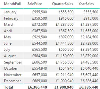
Figure 13-9.
The quarter- and year-to-date functions in DAX
As you can see, you have each month’s sales figures along with the cumulative sales for each quarter to date (and restarting each quarter). The final column shows you the yearly sales total for each month to date. Also, note that the months appear in calendar order, because the MonthFull field has used the MonthNumber field as its Sort By column.
Conceptually, the three functions that are outlined—TOTALMTD()
, TOTALQTD(), and TOTALYTD()—can be considered as CALCULATE() functions that have been extended to deliver a specific result for a time frame. You can always calculate aggregations for a period to date using the CALCULATE() function if you want to. However, since this “shorthand” version is so practical and easy to use, I see no reason to try anything more complicated when there is no real need.
Note
In this example, I suggest starting the process of adding a new measure with the Invoices table selected, merely because this table seems a good place to store the metric. You can create the metric in virtually any table in practice—provided that you have a coherent data model to build on.
Analyzing Data As a Ratio over Time
Looking at how data aggregates over time is only one of the ways that time intelligence can enable you to deliver time-based analysis
. On occasion, you may well want to see how a day’s sales relate to the total sales for a period. So in this example, we will calculate the daily percentage of sales for Brilliant British Cars relative to the total sales for the year 2014. The completed code for this slightly complex function is in step 21, should you prefer to type or copy and paste it.
- 1.In the Data View, select the InvoiceLines table and click New Measure.
- 2.Replace Measure with PercentOfYear.
- 3.To the right of the equals sign, enter (or type and select) SUM(.
- 4.Select the [SalePrice] field from the popup list of available fields.
- 5.Insert a closing parenthesis for the SUM() function.
- 6.Enter a forward slash to indicate division.
- 7.Enter (or type and select) CALCULATE(SUM(. This tells DAX that you want a filtered calculation and that the specific aggregation that you want to apply is a SUM() function.
- 8.Select the [SalePrice] field from the popup list of available fields.
- 9.Enter a right parenthesis to end the SUM() function.
- 10.Enter a comma. This tells the CALCULATE() function that you have chosen the aggregation that you want and will now apply a filter.
- 11.Enter (or type and select) DATESBETWEEN(.
- 12.Start typing the name of the date table (DateDimension) and then select the DateKey field from the popup. This tells the DATESBETWEEN() function which field in the time dimension should be used as its first parameter.
- 13.Add a comma. This ends the first parameter for the DATESBETWEEN() function.
- 14.Enter (or type and select) STARTOFYEAR(.
- 15.Start typing the name of the date table (DateDimension) and then select the DateKey field from the popup. This will be the lower boundary of the time span that will be used to filter the CALCULATE() function.
- 16.Add a right parenthesis to close the STARTOFYEAR() function.
- 17.Add a comma. This ends the second parameter for the DATESBETWEEN() function.
- 18.Enter (or type and select) ENDOFYEAR(.
- 19.Once again, start typing the name of the date table (DateDimension) and then select the DateKey field from the popup. This will be the upper boundary of the time span that will be used to filter the CALCULATE() function.
- 20.Add a right parenthesis to close the ENDOFYEAR() function.
- 21.Add two right parentheses. The first one ends the DATESBETWEEN() function, and the final parenthesis closes the CALCULATE() function. The formula should look like this:PercentOfYear = Sum([SalePrice]) / CALCULATE(SUM([SalePrice]),DATESBETWEEN(DateDimension[DateKey],STARTOFYEAR(DateDimension[DateKey]),ENDOFYEAR(DateDimension[DateKey])))
- 22.Press Enter or click the tick mark icon to complete the measure definition.
- 23.In the Modeling ribbon, click the percentage icon to format this measure as a percentage.
This formula was a little more intricate than those that you have seen so far in this chapter. So let me explain it in a bit more detail. At its heart, this formula consists of two main elements
:
- The sales total for the time element that will be used in a visualization. This could be the day, week, month, or quarter, for instance.
- The total sales for the entire year that will be used in a visualization. This has to be calculated independently of the actual date element that will be displayed. Consequently, the CALCULATE() function is used to extend the aggregation—the SUM() in this case—to the whole year. This is done by setting a range of dates as the filter for the aggregation. The date range is set using the DATESBETWEEN() function . This requires a lower threshold (defined by the STARTOFYEAR() function ) and a higher threshold (defined by the ENDOFYEAR() function). This way, the date range runs from the first to the last days of the year.
Finally, the calculation divides the specified time span’s total by the total for the year; the percentage for that sales period is displayed.
So that you can see the outcome of your formula, you could create a table that contains the following three fields
:
- FullDate
- SalePrice
- PercentOfYear
You should see something like Figure 13-10 if you have applied a page-level filter
to restrict the FullYear field to 2014, as described in the previous example.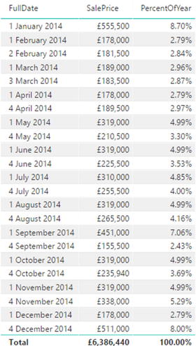
Figure 13-10.
Displaying the sales per day as a percentage of the yearly sales
You may be thinking that this was a lot of work just to get a percentage figure. Well, perhaps it is at first. Yet you can now capitalize on your effort and see how time intelligence is worth the effort. For instance, if you replace the DateKey field with the MonthFull field
in the table shown in Figure 13-9, you instantly see the sales percentages for each month. The same applies if you replace MonthFull with Quarter. You can see both these outputs in Figure 13-11. This is because you have created an extremely supple and fluid formula that can adapt to any time segment. The formula says to “Take the time segment (day, month, quarter, or year) and then find the date range for the whole year. Use this to calculate the total for the year, and then divide the figure for the time span by this total to display the percentage.”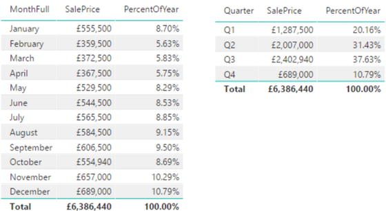
Figure 13-11.
Reusing a DAX time formula
Comparing a Metric with the Result from a Range of Dates
Let’s push the time-based data analysis a little further and imagine that you need to look at how figures have evolved compared to a specific time interval in the past. By this I mean that you want to see how sales for the current month have fluctuated compared to, say, the previous month. The following formula (that you can see in full in Step 14) shows you how to do just this. Once you understand the principles that this technique can be extended to, compare the data over many different time spans.
- 1.In the Data View, select the InvoiceLines table and click New Measure.
- 2.Replace Measure with PercentOfPreviousMonth.
- 3.To the right of the equals sign, type or select SUM(.
- 4.Type a left bracket and select the [SalePrice] field from the popup list of available fields.
- 5.Enter a right parenthesis to end the SUM() function.
- 6.Enter a forward slash to indicate division.
- 7.Enter (or type and select) CALCULATE(SUM(.
- 8.Select the [SalePrice] field from the popup list of available fields.
- 9.Enter a right parenthesis to end the SUM() function.
- 10.Enter a comma. This tells the calculate function that you have chosen the aggregation that you want; it will now apply a filter.
- 11.Enter (or type and select) PREVIOUSMONTH(.
- 12.Start typing the name of the date table (DateDimension) and then select the DateKey field from the popup. This tells the PREVIOUSMONTH() function the time dimension field that should be used as its parameter.
- 13.Enter a right parenthesis to end the PREVIOUSMONTH() function.
- 14.Enter a right parenthesis to end the CALCULATE() function. The formula should look like this:PercentOfPreviousMonth = SUM([SalePrice]) / CALCULATE(SUM([SalePrice]), PREVIOUSMONTH(DateDimension[DateKey]))
- 15.Press Enter or click the tick mark icon to complete the measure definition.
- 16.Format the measure as a percentage.
Figure 13-12 shows you the output that can be obtained by using the MonthFull field to give the month of a year (2014 in this example) alongside the PREVIOUSMONTH() function. To stress that time intelligence can adapt to different circumstances, you can also see the PERCENTOFYEAR function from the previous example—only it has automatically returned the percentage for the month this time.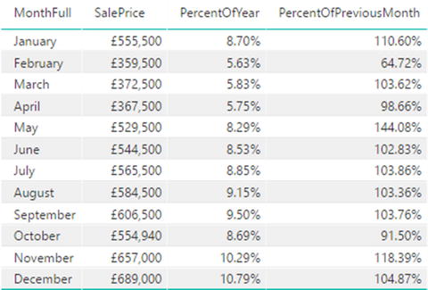
Figure 13-12.
Comparing values with a previous period of time
Once again, the “magic” in the formula was the use of the CALCULATE() function. Yet again, this function required you to enter two elements:
- An aggregation to carry out (the sum of the Sale Price in this case).
- A filter to apply (the previous month in this example). Once again, the function uses the date key from the date table to apply the time intelligence.
With these two parameters in place, DAX was able to take the time element used in the visualization (the month) and say, “Give me the aggregation for the previous month.”
Comparisons with Previous Time Periods
While the various DAX functions that return a “previous” time span are extremely useful, it could be argued that they are a little rigid for some types of calculation. After all, comparisons to the previous month typically require you to display data by month. So DAX has alternative methods of comparing data over time that do not require you to specify exactly which time element (day, month, quarter, or year) you want to compare with. Instead, you can merely say that you want to go back a defined period in time, and then depending on the choice of time element that you use in a visualization, DAX automatically calculates the correct figure for comparison.
Calculating Sales for the Previous Year
As a first example, let’s imagine that you want to compare current sales with sales for the current period—be it a day, week, month, quarter, or year. There might be several ways of doing this, but there is one fairly simple approach that returns the total car sales for the same time span for the previous year. Once the principle is clear, I will show you how to extend this to calculate the following:
- The average car sales price for the previous year
- The number of cars sold in the previous quarter
Initially, you should carry out the following steps to calculate sales
for the previous year (see step 14 for the complete formula):
- 1.In the Data View, select the Invoices table and click New Measure.
- 2.Replace Measure with PreviousYearSales.
- 3.To the right of the equals sign, enter (or type and select) CALCULATE(.
- 4.Enter (or select) SUM(.
- 5.Select the InvoiceLines[SalePrice] field.
- 6.Enter a right parenthesis to close the SUM() function.
- 7.Enter a comma.
- 8.Enter (or select) DATEADD(.
- 9.Select the DateDimension[DateKey] field. This indicates to DAX the correct date table and date key field.
- 10.Enter a comma.
- 11.Enter -1. This will cause the time comparison to apply to a previous period of time.
- 12.Enter a comma.
- 13.Enter (or select) YEAR. This indicates to the DATEADD() function that it wants to compare figures with the previous year.
- 14.Enter two right parentheses. The first one closes the DATEADD() function; the second one closes the CALCULATE() function. The formula will look like this:PreviousYearSales = CALCULATE(SUM(InvoiceLines[SalePrice]), DATEADD(DateDimension[DateKey],-1,YEAR))
- 15.Press Enter or click the tick icon in the formula bar to finish the measure.
- 16.Format the measure appropriately.
Figure 13-13 shows how the sale price (at the quarter level in this instance) is compared to last year’s sale price when you add the PreviousYearSales measure to a table. In this example, the table shows only sales for 2014. Consequently, the previous year’s sales are those for 2013. What is so impressive is that if you filter the table on another year (2015 for example), you will see that the previous year’s figures are now those for 2014.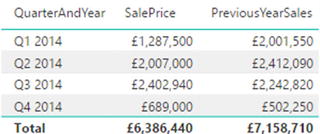
Figure 13-13.
Calculating metrics for a previous year
The formula sums or averages
the data in a column, but only for the previous year, compared to the date field for each row. (This is the InvoiceDate in the sample data, because the date field is linked to the date table in the sample data model.) Note that you do not use the InvoiceDate field in these formulas. This is because it is the field that is linked to the DateKey field of the date table. Power BI Desktop knows which field to use in the Stock table as the basis for time comparisons. To labor the point, it was essential to create a coherent and complete data model to make time intelligence work perfectly.
In this example, you set the “time shift” to a negative value, so that DAX would go back one year in time. You can also use positive numbers if you are looking at data from a past viewpoint and want to compare with data from later dates.
Tip
The DATEADD() function lets you replace YEAR with MONTH or DAY if you need to compare with data from days or months previously.
Once you have mastered this technique, you can extend and enhance a formula such as this to provide a multitude of metrics that will adapt to the time-based filters on tables and charts. As a second example, try creating the following measure. It will calculate the average sale price for the selected period(s) in the preceding year. I hope that by now you have become used to writing DAX formulas, so I will not explain how to create this formula, step by step. Instead, I will let you create it unaided. This should provide you with some good practice in creating DAX formulas by yourself.
AverageSalePricePreviousYear = CALCULATE(
AVERAGE(InvoiceLines[SalePrice]),
DATEADD(DateDimension[DateKey],-1,YEAR)
)
Note
I have formatted the code in this example for greater readability on the page and hopefully to make the logic of the functions more comprehensible. You might not be able to use the code formatted like this in Power BI Desktop without simplifying the presentation.
Alternatively, perhaps you want to see the number of sales
for the previous quarter relative to the date that is used to filter a visualization. This formula would be as follows:
NumberOfSalesPreviousQtr = CALCULATE(
COUNT(InvoiceLines[InvoiceID]),
DATEADD(DateDimension[DateKey],
-1,QUARTER)
)
Now that you have seen the principle, you are free to adapt it to your specific requirements. You can use any of the DAX aggregation functions that were described in the previous chapter. You can mix these with the four interval types (Year, Quarter, Month, and Day) that the DATEADD() function uses to deliver a truly wide-ranging set of time comparison metrics that automatically adapt to the time span of your Power BI Desktop visualization.
Comparison with a Parallel Period in Time
Looking at metrics from the past can be a key indicator of how a business is progressing. Clearly identifying the extent (or lack of) progress is even more telling. There are several ways that you can perform these types of calculation in DAX. In this section, you will see a couple of techniques that you may find useful.
Comparing Data from Previous Years
The following two measures (YearOnYearDelta and YearOnYearDeltaPercent) calculate the increase or decrease in sales compared to a previous year and also that change expressed as a percentage. These measures extend the logic of the last few formulas using functions that you have already met. I will presume that after two chapters on DAX, you do not really need a step-by-step explanation on how to enter a formula
. So I will only present and then explain the code from now on. The following is the code to add YearOnYearDelta and YearOnYearDeltaPercent as new measures to the Invoices table:
YearOnYearDelta=IF(
ISBLANK(
SUM(InvoiceLines[SalePrice])
),
BLANK(),
IF(
ISBLANK(
CALCULATE(
SUM(InvoiceLines[SalePrice]),
DATEADD(DateDimension[DateKey],
-1, YEAR)
)
),
BLANK(),
SUM(InvoiceLines [SalePrice])
- CALCULATE(
SUM(InvoiceLines[SalePrice]),
DATEADD(DateDimension[DateKey], -1, YEAR)
)
)
)
YearOnYearDeltaPercent=IF(
ISBLANK(
SUM(InvoiceLines[SalePrice])
),
BLANK(),
IF(
ISBLANK(
CALCULATE(
SUM(InvoiceLines[SalePrice]),
DATEADD(DateDimension[DateKey],
-1, YEAR)
)
),
BLANK(),
(
SUM(InvoiceLines[SalePrice])
- CALCULATE(
SUM(InvoiceLines[SalePrice]),
DATEADD(DateDimension[DateKey],
-1, YEAR)
)
)
/CALCULATE(
SUM(InvoiceLines[SalePrice]),
DATEADD(DateDimension[DateKey],
-1, YEAR)
)
)
)
These two formulas are a lot easier than they look, believe me.
The formula for YearOnYearDelta is this:
SUM(Stock[SalePrice])
- CALCULATE(SUM(InvoiceLines[SalePrice]), DATEADD(DateDimension[DateKey], -1, YEAR))
All the code says is “Subtract last year’s sales
from this year’s sales.” Everything else is wrapper code to prevent a calculation if either this year’s or last year’s data is zero.
Equally, this is the core code for the YearOnYearDeltaPercent formula:
SUM(InvoiceLines[SalePrice]) - CALCULATE(SUM(InvoiceLines[SalePrice]),DATEADD(DateDimension[DateKey], -1, YEAR)) / CALCULATE(SUM(InvoiceLines[SalePrice]),DATEADD(DateDimension[DateKey], -1, YEAR))
In other words, “Subtract last year’s sales from this year’s sales and divide by last year’s sales.” Everything else in the complete formula that is given in full earlier exists to prevent divide-by-zero errors or unwanted results for the first year where there is no previous year’s data!
The logic “wrapper” around the core formula uses two new functions:
- ISBLANK(): This function tests if a calculation returns nothing and allows you to specify what to do if this happens. This is a bit like an IF() function that only tests for blank data.
- BLANK(): Returns a blank (or Null). This is useful for overriding unwanted results and replacing them with a blank.
Using these functions lets you handle the case where there is no data for a previous period of time. Because you are using the
ISBLANK() function
to test for inexistent data, you are able to replace any missing data with a BLANK()—rather than letting Power BI Desktop display an unsightly error.
We have seen a couple of fairly complex formulas in a short section. So I think that it is a good idea to see how they look when you apply them. In this case, I will use a Power BI Desktop table to show the results, as shown in Figure 13-14. As you can see, the appropriate formats have been applied to each metric to enhance readability.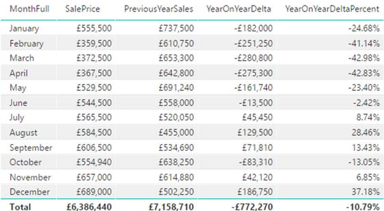
Figure 13-14.
Power BI Desktop output for year-on-year comparisons
Once again, these formulas only scratch the surface of the myriad possibilities that DAX has on offer. However, you can adapt them to create comparisons by quarter, month, or day if you prefer simply by changing the specified time interval from YEAR to QUARTER, MONTH, or DAY.
Comparing with the Same Date Period from a Different Quarter, Month, or Year
In the last couple of sections, you saw various ways to compare data from a prior year or month. DAX offers one alternative method for these kinds of calculations that can be both easy to implement and extremely powerful. Moreover, it can serve as the basis for comparison with years, quarters, or months. This is the PARALLELPERIOD() function
. Suppose that you want to use it to find average sales for the previous quarter.
Because this function is fairly similar to the DATEADD() function that you saw previously, I will not explain it step by step; instead, I prefer to give you three examples of measures that you can add to the InvoiceLines table directly.
Here are the sales for the preceding month:
SalesPrevMth = CALCULATE(SUM(InvoiceLines[SalePrice]), PARALLELPERIOD(DateDimension[DateKey],-1,MONTH))
Here are the sales for the preceding quarter:
SalesPrevQtr = CALCULATE(SUM(InvoiceLines[SalePrice]), PARALLELPERIOD(DateDimension[DateKey],-1,QUARTER))
Here are the sales for the preceding year:
SalesPrevYr = CALCULATE(SUM(InvoiceLines[SalePrice]), PARALLELPERIOD(DateDimension[DateKey],-1,YEAR))
You see two examples of these functions displayed as simple visualizations in Figure 13-15.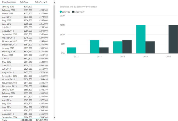
Figure 13-15.
Using the PARALLELPERIOD() function
Note
You need to be aware that the PARALLELPERIOD() function
compares the current data, not just up to the same data in the previous period (be it a year, a quarter, or a month), but for the entire previous time period.
There are further DAX functions that you can also use when comparing data over time. These are outlined in Table 13-7.
Table 13-7.
DAX Date and Time Formulas to Compare Values over Time
Formula
|
Description
|
Example
|
|---|---|---|
PARALLELPERIOD()
| Finds dates from a “parallel” timeframe defined by a certain number of set intervals. The first parameter is the source data; the second is the number of years, quarters, months, or days; and the third is the definition of the interval: years, quarters, months, or days. A positive number of intervals looks forward in time and a negative number goes backward in time. |
CALCULATE(SUM(InvoiceLines[SalePrice]), PARALLELPERIOD(DateDimension[DateKey],-1,MONTH))
|
SAMEPERIODLASTYEAR()
| Finds the date(s) for the same time range one year before. |
CALCULATE(SUM(InvoiceLines[SalePrice]), SAMEPERIODLASTYEAR (DateDimension[DateKey))
|
DATEADD()
| Used to return data from a past or future period in time compared to a specified date. The date difference can be in years, quarters, months, or days. |
CALCULATE(SUM(InvoiceLines[SalePrice]), DATEADD(DateDimension[DateKey], -1, YEAR))
|
DATESBETWEEN()
| Calculates a list of dates between two dates. The first parameter is the start date and the second parameter
is the end date. |
DATESBETWEEN(Stock[PurchaseDate], Invoices[SaleDate])
|
DATESINPERIOD()
| Calculates a list of dates beginning with a start date for a specified period. |
DATESINPERIOD(DateDimension[DateKey],
DATE(2015,06,30),-90,day))
|
Rolling Aggregations over a Period of Time
We are now getting into the arena of more complex DAX formulas. So, since returning the rolling sum (or average) of a specified period to date necessitates several DAX functions and some in-depth nesting of these functions, I will take this as an example of a more complicated DAX formula. I will begin by outlining some of the functions that are used to deliver a result that is reliable and efficient:
- DATESBETWEEN() : Lets you select a range of dates. The three parameters are the date key field from the date table, then the starting date, then the ending date.
- FIRSTDATE() : Allows you to get the first date from a range. Since we are using this momentarily to go back a defined number of months, it will get the first day of the month.
- LASTDATE() : Allows you to get the last date from a range. Since we are using this momentarily to go back a defined number of months, it will get the last day of the month.
You can now create two measures (3MonthsToDate
and Previous3Months
) using some fairly sophisticated logic to ensure that only blank cells are returned if there is no previous year’s data using the following formulas:
3MonthsToDate=IF(
ISBLANK(SUM(InvoiceLines[SalePrice])),
BLANK(),
CALCULATE(
SUM(InvoiceLines[SalePrice]),
DATESINPERIOD(
DateDimension[DateKey],
LASTDATE(DateDimension[DateKey]),-3,MONTH
)
)
)
Previous3Months=IF(
ISBLANK(
CALCULATE(
SUM(InvoiceLines[SalePrice]),
DATEADD(DateDimension[DateKey],-1,MONTH)
)
),
BLANK(),
CALCULATE(
SUM(InvoiceLines[SalePrice]),
DATESBETWEEN(
DateDimension[DateKey],
FIRSTDATE(DATEADD(DateDimension[DateKey],
-4,MONTH)),
LASTDATE(DATEADD(DateDimension[DateKey],
-1,MONTH))
)
)
)
The 3MonthsToDate formula essentially evaluates the code that is in boldface. This says, “Add up the sales for a time period ranging from three months ago to now,” using the InvoiceDate field as the date to evaluate. The IF() function detects if there are sales for the current date, and if there are none (ISBLANK), then the calculation is not attempted, and a BLANK is returned.
The Previous3Months formula
is pretty similar, except that the time span uses the
DATESBETWEEN() function
to set a range of dates—from the first day of the month four months ago to the last date in the preceding month.
DAX contains a couple of functions that you can use to return a specific date when aggregating data over time. These are shown briefly in Table 13-8.
Table 13-8.
DAX Date and Time Formulas to Return a Date
Formula
|
Description
|
Example
|
|---|---|---|
FIRSTDATE()
| Finds the first date that an event took place. |
FIRSTDATE(Invoices[InvoiceDate])
|
LASTDATE()
| Finds the last date that an event took place. |
LASTDATE(Invoices[InvoiceDate])
|
Conclusion
This chapter has taken you on a concise tour of some of the ways that you can use DAX in Power BI Desktop to extract meaning from your data by analyzing its evolution over time.
First, you saw how to extract date and time elements from columns that contain dates. The new columns that you create based on dates can then be used to filter or group data in your visualizations. This way you can provide a daily, weekly, monthly, quarterly, and yearly breakdown of your source data. These date elements can also help you to filter the datasets that you are using by dates, date elements, and date ranges.
Then you saw how to prepare the dataset for time intelligence by adding a date table and joining this table to the other tables in the data model. Finally, you saw how to start adding formulas to the dataset to prepare all the time-based metrics that your Power BI Desktop reports could need. This can include analyzing sales to date or comparing data from previous time periods with current data.
Explaining all the possibilities of DAX would take an entire book, so all I wanted to do in this and the previous two chapters was explain how you can use core DAX functions in a handful of useful calculations. I sincerely hope that this brief overview helps you on your road to mastery of DAX and that you are able to apply these formulas to deliver stunning visualizations using Power BI Desktop.
Your data is now ready for output. It can be used as the basis for multiple dashboards and reports. This is the subject of the next six chapters.