13

Cost Control

Major topics in this chapter are cost control tools:

• Earned Value Analysis
• Milestone Analysis

These tools are designed to help you successfully perform cost control of the project. More precisely, they help you get a handle on revised cost estimates, budget updates, and forecasts of final cost (see Figure 13.1). In the process, you will rely on cost baseline and information about project plan execution, while synchronizing cost control tools with the tools of scope and schedule control and facilitating processes. Together, these tools should enable you to report performance in the ongoing march toward project closure. The objective of this chapter is to offer practicing and prospective project managers the following learning opportunities:

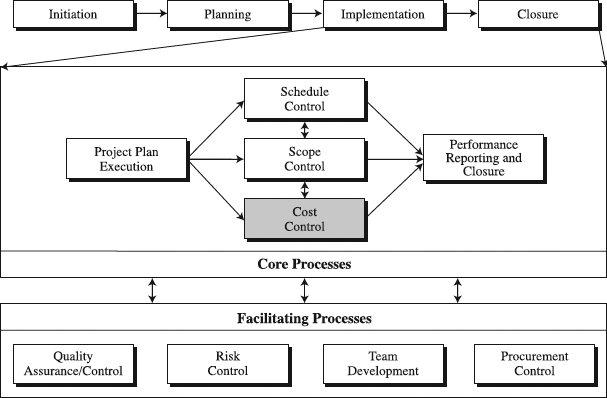
Figure 13.1 The role of cost control in the standardized project management process.

• To become familiar with cost control tools in the proactive cycle of project control
• To choose a cost control tool that matches their project situation
• To customize the tool of their choice

These skills are vitally important in implementing a project and building the standardized PM process.

Earned Value Analysis

What Is Earned Value Analysis (EVA)?

Earned Value Analysis periodically records the past of a project in order to forecast its future (see Figure 13.2). During progress statusing, EVA measures a project's schedule and cost performance to find out whether they are ahead or behind the plan (schedule and cost variances) and why. Then, final project costs (estimate at completion) and completion date (schedule at completion) are predicted. While the practical elegance of such an approach comes from EVA's seamless integration of project scope, cost, and time, its special value is in the proactive, predictive approach. In particular, these predictions warn us of possible problems, creating opportunities to fix them in a timely manner and keep the project on its planned course. In summary, EVA strives to establish the accurate measurement of physical performance against a plan to enable the reliable forecast of final project costs and completion date [1]. In this chapter, we describe the deliberate sequence of several steps to help explain the conceptual simplicity of performing EVA. For further understanding, refer to the box that follows, “Basic Earned Value Analysis Terminology.”

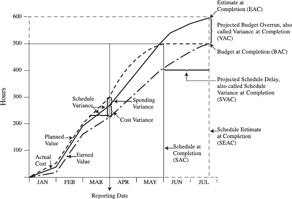
Figure 13.2 An Earned Value Analysis chart.

Performing Earned Value Analysis

First conceptualized by the industrial engineers of the late nineteenth century, EVA grew to its comprehensive and dominant form under the auspices of the government PM [3]. In the process of growth, the original simple terminology of the engineers yielded to a confusing terminology. Although EVA has become an effective tool, primarily in large government projects, it has not been able to attract a large following in the private sector. The business world nowadays is generally made up of small and medium projects, often managed by companies that have started using the PM approach recently [4]. These companies need EVA in a simpler form, built on a terminology as simple as that of the industrial engineers and often based on resource hours as much as on dollars. Stellar, although rare examples of private organizations pursuing such EVA can be found in the industry [5]. Fully valuing both approaches, for large government and smaller private projects, we will first focus on a comprehensive approach and then in the customization section offer suggestions for the establishment of simpler forms of EVA.

Collect Necessary Inputs. To be effective, EVA has to be set on some firm foundations. These are essentially inputs such as

• Fully defined project scope
• Project schedule
• Time-phased budget.

Fully defining the project scope is, of course, not an easy task, especially when you are dealing with a new job fraught with unknowns. Among the available tools for scope definition, it is our belief that the logic of systematic decomposition of project work into successive levels of manageable chunks of work, as in WBS, provides a sufficient degree of confidence that the scope will be fully defined, including all work to do in the project. This is why one of the golden rules of the WBS structuring is to show all project work. That this is critical becomes clear when we know that EVA may require an estimate of the percent of work completed. If the estimate is 20 percent complete and the project scope is not fully defined, the estimate is apparently inaccurate, because it does not refer to the full scope of work. A disciplined and appropriate application of WBS can help create a reasonable representation of a fully defined project scope.

WBS provides a basis for scheduling the project scope. Each task will be carefully analyzed to determine when in the project time line it will be executed. Details about beginning and ending points of work tasks, as well as their durations, will be determined in the schedule. Such information, along with the approved budgets for tasks, essentially defines scheduled work or planned value. As the project implementation unfolds, physically completed work is evaluated and earned value determined. Both the plan value and earned value are derived from the project schedule information and are critical for successful EVA. For that reason, the project schedule is a critical input to EVA.

A fully defined project scope that is scheduled for implementation must be based on careful resource estimates. Specifically, resources to complete each WBS element need to be identified and allocated for certain time periods on the schedule. This creates a time-phased budget of resources. These resource estimates along with the scheduled work help generate the planned value. Also, these estimates combined with the completed work constitute the earned value. Apparently, the time-phased budget is a critical input to EVA. In summary, EVA requires a fully defined project scope integrated with allocated resources, all translated into a sound project schedule for performance. Often these three inputs are termed a “bottom-up project baseline plan” [6].

Set Up a Performance Measurement Baseline (PMB). You will establish a PMB in order to determine how much of the planned work you have accomplished as of any point in the project time line. Establishing a PMB involves three tasks:

• Determining points of management control and who is responsible for them
• Selecting a method for measurement of earned value
• Setting up a PMB

The foundation for the tasks is the project baseline plan, which fully defines project scope, integrating it with allocated resources and translating them into a project schedule for performance, all within the framework of WBS. Given that WBS has elements on multiple levels, you have to decide which elements (on which level) will be management control points. These points are called control account plans (CAP). Although at first sight this might seem a confusing term, in actuality its concept is simple—a CAP is a basic building block of EVA, a point at which we measure and monitor performance. The makeup of a CAP is defined in the box that follows, “Key Components of a Control Account Plan.”

CAPs may be located on a selected level of a WBS—at level 1, or 2, or 3 (the project is level 0 of WBS), or all the way down to whatever is chosen as a lowest level to exercise management control. The essence is that a CAP is a homogeneous grouping of work elements that is manageable, which brings us to the issue of its size. How large or how small should a CAP be? According to the current trends in private industry, the size of CAPs is on the increase [1]. One reason is that, not surprisingly, project managers want to concentrate on CAPs that includes larger work elements, which are typically on higher levels of the WBS. Also, they include into a CAP all organizational units responsible for its constituent work elements. The desired result of these trends is to enable project managers to focus their attention on fewer but more vital control points of their projects, making EVA significantly easier to use and much more time-efficient. Such a CAP, then, has a clearly defined narrative scope, location in the WBS, constituent work elements, timeline, and budget. Although the budgets are often expressed in dollars (usually in large projects), they come in all forms—from resource hours to units to standards. Because so many project managers manage only resource hour budgets, we will use the hours in our examples. To ensure accountability for the budgets, each CAP should be assigned to a person responsible for its performance. Figure 13.3 displays an example of a CAP.

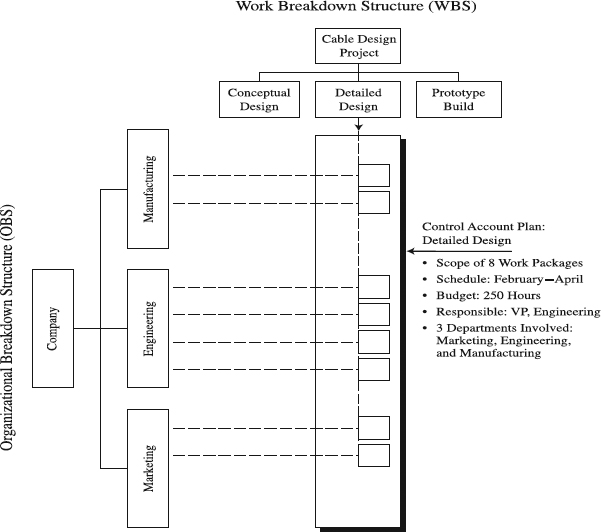
Figure 13.3 Forming a control account plan.

From Project and Program Risk Management: A Guide to Managing Project Risks and Opportunities, Max R. Wideman, ed., Newtown Square, PA: Project Management Institute, Inc., 1992. All rights reserved

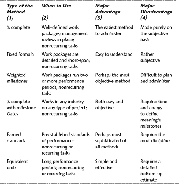
Measurement of a CAP's performance, the cornerstone of the whole EVA, calls for well-defined methods of measurement. While we review several such methods (see Table 13.1), hard-and-fast rules for selecting the appropriate one do not exist. Rather, the choice you have to make is a personal one, often arbitrary, and may vary on a project-by-project basis. In the selection process, the project team and CAP managers should focus on the ease and accuracy of measurements that can be consistently applied to appropriately support their specific project needs.

The percent complete method uses a periodic—e.g., monthly or weekly—estimate of the percentage of completion of a work package, expressed as a cumulative value (e.g., 65 percent) against the full 100 percent value of the work package. Hailed as a simple and fast method, which perhaps explains its wide popularity, the method has also been viewed as being overly subjective. Defining work packages' scope well and checking on accuracy of the estimates helps make the subjectivity reasonable.

Table 13.1: Fundamentals of Major Earned Value Measurement Methods

Fixed formula by work package includes various options: 25/75, 50/50, 75/25, and so on. For example, 25/75 formula means that when a work package is started, 25 percent of the package's budget is earned, while the completion of the package earns another 75 percent. Apparently, any combination that adds up to 100 percent is possible. This is a quick way of estimating, applicable in situations where work packages are short-span and performed in a cascade type of time frame. It can also be accurate (see the box above, “50/50 Formula Offers Reasonable Accuracy.”

Weighted milestones is a method of dividing a long-span work package into a several milestones, each one assigned a specific budgeted value, which is earned when the milestone is accomplished. As objective as it is, the method's success hinges heavily on the ability to define meaningful milestones that are clearly tangible, budgeted, and scheduled.

Percent complete with milestone gates strives to balance the ease of percent complete estimates with the accuracy of tangible milestones. A work package of, say, 600 hours is broken down into three sequential milestones, each budgeted at 200 hours and placed as a performance gate. You are allowed to estimate the first milestone's earned value by percent complete up to 200 hours. To go beyond the point of 200, you need to meet predefined completion criteria for the first milestone. This procedure is repeated for subsequent milestones [1].

Earned standards is a method often applied by industrial engineers to establish planned standards for performance of work packages, which are then used as the basis for budgeting the packages and subsequently measuring their earned value. For example, the planned standard for producing a cup of lemonade at $0.20/cup is used to budget the work package including the production of 1,000 cups for $200. When 500 cups are produced, regardless of the actual cost the earned value is 500 cups X $0.20/cup = $100. Widely applied in repetitive types of project work, the method's foundations are the planned standards developed from historical cost data, time, and motion studies [1].

In equivalent completed units, a planned work package is earned when it is fully completed. Similarly, a planned portion of it is earned when completed. For example, a work package to build 5 miles (five units) of freeway is estimated at $3M/mile for a total of $15M. It is fully earned when all five miles are finished. Also, the completion of half a mile will earn $1.5M. Based on detailed bottom-up estimates, the method is favored by the construction industry without ever having been called its real name—the earned value.

After this short review of the six methods, two things need to be mentioned in closing comments about the task of measuring EVA performance. First, note that the work package is the place where the measurement is taken, while measurement for a CAP is a summation of work packages' measurements. Second, there is no single best way to measure earned value for any type of project task. This contingency rule means that different types of tasks will use different methods, and perhaps the most appropriate method is to combine multiple methods, relying on CAP managers to collectively estimate the earned value of individual work packages. For an example of a project where multiple methods are used, see Figure 13.5a. A design project consists of three CAPs, essentially three phases on level 1 of WBS. Each of them applies a different method of EVA measurement—percent-complete, weighted milestones, and earned standards. Since each CAP consists of multiple work packages, this means that all work packages within the CAP are measured with the same method. As we remind you that the EVA measurement method is the last on the list of components of a CAP (see the previous box, titled “Key Components of a Control Account Plan), we move to establish the PMB.

The PMB is a time-phased sum of detailed and individually measurable CAPs. What is included into CAPs depends on how companies define cost management responsibilities of their project managers. Many companies allow their managers of internal projects to manage only direct labor hours, which is our focus here. In that case, their CAPs and PMB will include only direct labor hours. On the other end of the spectrum are project managers whose job is to manage all project costs, as well as management reserves and profit. Accordingly, their PMB will reflect this situation. Still other companies may select that their PMB and related cost responsibilities of project managers is somewhere between the two ends of the spectrum.

In projects with lower uncertainty, a firm PMB with detailed CAPs can be established before the project implementation begins. What if you have to start executing an uncertain project in which front-end CAPs are detailed out while the later ones cannot be planned for the lack of information (see Figure 13.4)? And, what if a CAP's scope starts changing? The answer for the first issue is the rolling wave approach; as you progress in executing the available detailed CAPs, you will generate more information that enables you to plan other CAPs [7]. As for the second issue of scope changes, you should establish a PMB change control procedure. By carefully handling all changes to the scope, you will be able to update and maintain the approved PMB, a prerequisite to successful EVA.

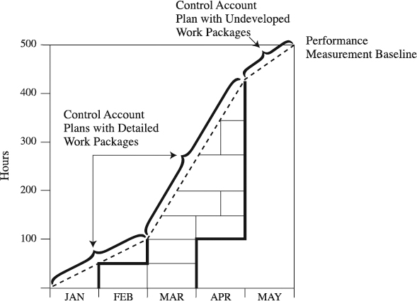
Figure 13.4 Performance measurement baseline: the sum of control account plans.

From Earned Value Project Management, Second Edition, Quentin W. Fleming and Joel M. Koppelman. Newtown Square, PA: Project Management Institute, Inc., 2000. All rights reserved.

For practical purposes of EVA, the time-phased PMB can be displayed as a cumulative performance curve representing the planned value over the project schedule. That is the curve shown in Figure 13.5b, developed for a design project whose performance data is given in Figure 13.5a. In summary of this step, a project's PMB is now in place, consisting of detailed CAPs, each one essentially a form of subproject.

Evaluate Project Results. This step compares the actual results of performing the project with its plan (PMB) following the proactive cycle of project control (see the box “Five Questions for PCPC for Cost Control” later in this chapter). While the very measurement of performance occurs within individual CAPs, you may monitor and periodically (weekly or monthly) evaluate performance results at three levels: within individual CAPs, at some intermediary summary level (either a WBS element beyond the CAP or an organizational breakdown structure level), and at the project level. This step includes the following:

• Focus on schedule area: evaluate schedule variance (SV) and schedule performance index (SPI).
• Focus on cost area: evaluate cost variance (CV) and cost performance index (CPI).
• Identify the cause of the variances, if any.

Our example in Figure 13.5c shows the comparison—the cumulative performance curve for actual values against the performance curve for planned values. To tell the truth, the majority of project managers, despite its potentially deceptive results, favors this traditional cost management approach. At the end of March in our example, the difference between the two curves—called the spending variance—only reflects whether the project stays within the approved budgeted hours. In does not in any way determine the project's true cost performance status. If used for establishing the project's true cost performance status in Figure 13.5c, the comparison would mislead us by indicating that the actual performance is under budget (300 hours − 270 hours = 30 hours), a positive development. This couldn't be further from the truth—the project is in cost trouble, as we will see soon, and that can't be discerned using this planned-versus-actual approach. The reason for this false finding is in comparing points on the planned and actual curves that include different scopes of work. In short, apples are compared with oranges. Another trouble with this two-dimensional traditional approach from Figure 13.5c is in that it relates to cost only. To get an insight into the project schedule performance, we need a separate planned versus actual schedule chart, and that one would not match the cost chart from Figure 13.5c. The remedy for these problems is a chart that integrates true cost and schedule performance. This is where the earned value performance curve steps in, as illustrated in Figure 13.5d.

A comparison of the earned and planned value at the end of March indicates the following:

This negative SV means that the project falls behind its planned work. A look back at Figure 13.5d reveals two manifestations of the same SVs—one drawn vertically is expressed in hours (budget units), the other horizontal in time units. Not surprisingly, you may prefer the one expressed in time units (days, weeks, months). It is generally easier to identify such time units of delay by means of the schedule performance index. Before we get there, it is worth mentioning that anytime SV is negative, the project is late to its planned work, and anytime SV is positive, the project is ahead of its planned work.

Another task in evaluating the schedule position is calculating SPI. At the end of March in Figure 13.5d, the situation is as follows:

SPI quantifies how much actual earned value was accomplished against the originally planned value. In other words, it represents how much of the originally scheduled work has been accomplished at a certain point of time [1]. An SPI equal to 1 means perfect schedule performance to its plan. Any SPI greater than 1 implies an ahead-of-schedule position to the original plan of work. SPI running below 1 reflects behind-schedule position to the originally scheduled work. Therefore, our SPI of 0.75 indicates that 75 percent of the originally planned work is accomplished. This means our project is way behind, more precisely, 25 percent (1 − 0.75 = 0.25) behind the baseline plan of work. Since our reporting date at the end of March is the 90th day of the project, we can tell that our project is 22.5 days (25 percent of 90 days) behind the original plan of work.

Schedule analysis in EVA deserves a word of caution. Specifically, anytime you find a schedule delay condition that includes negative SV and SPI that is less than 1, you should know that EVA schedule variance is not based on the critical path information and may be deceptive. Poor schedule performance of some work packages or tasks may be balanced by schedule performance of other work packages or tasks. Use your critical path schedule and risk analysis in conjunction with EVA schedule analysis [8]. If the late work packages/tasks are on the critical path or are highly risky to the project, complete the work packages/tasks at the earliest possible date [1].

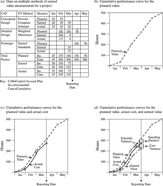
Figure 13.5 Performing Earned Value Analysis.

Now we can move to our second area of interest in this step—calculate cost variance (CV) and cost performance index (CPI). At the end of March in Figure 13.5d, CV is as follows:

and

The purpose of CV is to indicate the differential between the earned value for the physically accomplished work and the actual cost to accomplish the work. Therefore, the positive CV means that the project is running under budget, while negative CV signals the project is in the red, overrunning the budget. Our case is, apparently, experiencing the latter, consuming 45 more hours than we have allocated for the amount of accomplished work.

CPI is a cost efficiency factor. By relating the physically accomplished work to the actual cost to accomplish the work, CPI establishes the cumulative cost performance position. When CPI is equal to 1, that means perfect cost performance to its original budget. Values of CPI exceeding 1 indicate under original budget position, while those less than 1 spell the trouble of over original budget position. In our example, the CPI's reading of 0.83 is that earned value for the physically accomplished work is only 83 percent of the actual cost to accomplish the work. Put it differently, 17 percent (1 − 0.83 = 0.17) of actually consumed hours are a budget overrun. Why are there variances in our example? Identifying and understanding the root cause of the variance are the last task in this step of evaluating project results. The variances are so important that a careful dissection of the project is a necessary strategy to uncover the cause and, later, develop corrective actions.

Both CPI and SPI cumulative curves enable a very effective tracking of a project, as illustrated in Figure 13.6. Note that both rate and trend of the indices are crucial here. Key to it is using the cumulative data, rather than incremental data (weekly or monthly). Unlike the incremental data, which is prone to fluctuations, the cumulative data tends to smooth out the fluctuations and is very effective in forecasting the final project results, the focus of our next step.

Forecast the Final Project Results. If there is one single, most compelling reason to use EVA, it is for its proactive ability—the ability to reasonably forecast the final project results most of the time during project execution. We say most of the time because it is only somewhere at the 15 percent completion point and beyond that a sound, statistically reliable forecast becomes feasible by completing the following tasks:

• Forecast project's completion date.
• Forecast project's cost at completion of the project.
• Take corrective actions, if necessary.

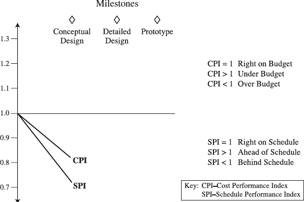
Figure 13.6 Tracking cumulative Schedule Performance Index (SPI) and Cost Performance Index (CPI).

A quick forecast of the completion date for our example in Figure 13.5d at the end of March is as follows:

This quick method may unfortunately turn risky. As mentioned earlier, an EVA schedule delay condition that like in our example has a negative schedule variance and SPI that is less than 1 is not based on the critical path information and may be deceptive. Therefore, a better solution is to predict the completion date based on results of the critical path analysis in combination with EVA schedule variance.

Out of 20+ available formulas to estimate a project's cost at completion of the project [1], we will only look at two that are frequently used. Here is the low-end formula and forecast:

This means that at the end of the project we would need 600 hours to get this project done, a whole 100 hours variance at completion (VAC) over the original budget. Clearly, this method—called constant cost efficiency rate—relies on to-date cost overrun and projects it to the end of the project. Figure 13.2 includes the prediction of the final results developed by means of the quick forecast for SAC and low-end formula for estimate at completion (EAC).

A more rigorous method, based on our forecast on both the cost overrun and schedule slippage to date, is called constant cost and schedule efficiency rate:

With this method, we get variance at completion of 300 hours. Some researchers found that the low-end forecast is a reliable measure of the “minimum” hours, while the high-end method produces a forecast of the “maximum” hours we may need [1]. Their claim that the high-end method is the most appropriate forecasting method should be contrasted with a recent study's finding that the low-end method is the most accurate [9]. With such differing views using both methods to develop a range of final cost projections, in our case between 600 and 800 hours, makes sense. This is the absolute essence of prediction—produce a sanity check of the trend and final direction of the project (for major factors impacting the final results, see the box that follows, “Three Factors Influencing the Final Project Results”). In our example, the prediction is not good; actually, it is very bad, but its ultimate value purely depends on the willingness of management to act or not to act. If the option is to not act, the whole EVA is meaningless—it has no value whatsoever. Choosing to act by developing corrective actions rooted in the root causes of the problems is what EVA is designed for.

Utilizing EVA

When to Use. EVA is a choice for any project, regardless of the industry and size. With the amount of resources at stake in large projects, a full-scale EVA can be easily justified. Simplified versions of EVA such as cost and achievement analysis (see the “Variations” section coming up in the chapter) are a right fit for smaller projects. In either case, a good measure of customization is recommended.

Time to Perform. Any project in need of EVA must establish the scope, budget resources, and schedule tasks. When that is available, small projects are ready to deploy simple versions of EVA. In such an environment, a project with ten tasks, 300 to 500 hours in budget, with some overlap of tasks may have several tasks to evaluate weekly. This would probably need no more than an hour to accomplish. The situation changes in large projects, where tens of hours may easily be expended to run a regular, full-scale EVA.

Benefits. A disciplined employment of EVA that is based on a clear understanding of what a company wants to accomplish with it offers multiple benefits. (see the box that follows, “Five Benefits of Earned Value Analysis”). We begin with how EVA can help handle a fundamental question in today's project business: Is the project on schedule, behind, or ahead of schedule? Using the schedule variance and SPI in conjunction with the critical path method can reliably answer this question. In a similar manner, the cost variance and CPI play the crucial role in establishing the true cost position of the project by finding whether it is on, over, or under budget.

Each true schedule and cost position may be viewed as a significant step, telling what happened in the project at a specific point of time of its history. Knowing that they cannot change the history, proactive project managers use the position to look into the future and impact it. In particular, research of the past use of EVA indicates that cumulative cost performance index for larger projects becomes very stable at the 15 percent completion point in the project [10]. Simply, this means that early in the project the cost performance index exhibits a consistent pattern, enabling reliable forecasts of the project cost at completion. Similarly, the schedule performance index combined with the Critical Path Method can be used for predicting the final completion date. Hence, you can periodically ask, “Given my current performance, what will be my final costs and completion date?” The answer offers trend performance and, if the trend differs from the baseline plan, an early-warning signal. This may be the highest value of EVA—providing project managers with the early-warning signal about possible problems in the future and serving them an opportunity to devise and take needed corrective actions while there is still time to fix such project problems. Most importantly, this works for smaller projects as well. According to some experts, smaller projects' accurate cost performance index readings necessary for trend performance and early-warning signals could become available at 10 percent completion in the project life cycle, even earlier than for larger projects [1].

The true credibility and, eventually, the value of EVA are rooted in its integration of project scope, schedule, and cost. WBS provides the vehicle for the integration of all project work through its hierarchical tree of deliverables called work elements. For each element with its scope of work, resources are allocated, schedule determined, and cost estimated. By measuring current and predicting future performance for each work element, and aggregating them up the WBS hierarchy, we can arrive at the measurement of the current performance and prediction of the future performance for the total project. This integrated and consistent manner of performance measurement and prediction [11] is a vital improvement compared to the traditional separate schedule performance and cost performance charts, a fairly typical approach in the industry. These are fraught with risks of having nonintegrated, multiple, and often conflicting measurements of performance.

Project managers focus on tasks that matter. To separate tasks that matter in controlling their projects from those that don't, they can use EVA, highlighting tasks that have the highest variances from the approved project baseline. These tasks become critical in ensuring that the project ends in line with the baseline. For that reason, project managers focus on such critical tasks, devoting them most of their attention and time. By doing that, they are managing by exception, putting their expertise to work where it is most needed. This certainly becomes easier with the establishment of thresholds for tasks—specific levels of schedule or cost variances that, if exceeded, trigger management action.

The assessment and improvement of efficiency and effectiveness of projects call for comparable, consistent, and transparent information about their results. This is not possible if this information comes from multiple systems, where one system is used for large projects and another for small projects, with project managers interpreting results in one way, senior mangers in another. These incompatible systems rid a company of the great opportunity to compare all its projects and opt to go for the most efficient and effective ones. A true alternative is a system in which the information comes from a single, universal yardstick for measurement of current performance and prediction of the future performance for all projects and all management levels. EVA provides such a universal system. For example, a comparison of the scheduled work with accomplished work produces a true indicator of whether a project is meeting time expectations set forth by management [1].

Advantages and Disadvantages. Advantages are that EVA is

• Conceptually simple. Although at first sight it may appear complex because of its three-dimensional makeup (planned, actual, earned), in essence, EVA is conceptually simple.
• Relatively easy to learn. Realistically, it does not take extensive training to get a handle on the EVA fundamentals. This is an advantage that should propel otherwise the low use of the tool.

Disadvantages are primarily in EVA's

• Low use. Some experts estimate that perhaps less than 1 percent of all projects, primarily including the major systems acquisitions by governments, deploy EVA [1]. The reasons may lie in its past history of application, plagued by confusing terminology and many rules and interpretations that governments as major users prescribe. This red-tape mentality might have scared many potential users away, creating an image of EVA as a government type of tool that is not useful for the private sector. With such a myth in circulation, many good companies missed the opportunity to customize the tool for their own project needs and enjoy numerous benefits.

Variations. There are several cost control tools that are conceptually founded on earned value, although they are not, at least explicitly, referred to as what they really are—a simplification of EVA. Two such tools that enjoy a high level of popularity are Milestone Analysis and cost and achievement analysis [12]. Overall, their appeal is in that they use simple terminology and straightforward procedure, which is perhaps why they are so time-efficient. Because of a perception in the PM community that the Milestone Analysis is a tool of its own, it is described as a separate tool in the next section in this chapter. The cost and achievement analysis that is briefly covered in the following is illustrated in Figure 13.7.

Based on the scope and schedule for a task, its budget (same as the planned value in EVA) of resource hours is defined. Multiplying the budget by the percent complete will produce the achieved value (equivalent to the earned value in EVA). Actual consumed hours (equivalent to actual cost in EVA) to complete the scope defined by the achieved value are recorded as well. Values for the budget, achieved, and actual cost are then used to predict the final cost for the task. Doing this on a regular basis for each task, in cumulative terms, allows you to sum them to produce budget, achieved, and actual values for the whole project and predict the project's final cost. The approach offers a great way to be proactive in smaller projects.

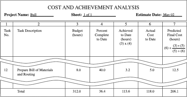
Figure 13.7 Cost and achievement analysis.

Customization. If EVA is such a good project performance measure and a trend predictor, why is it not used more in the private industry? In addition to already mentioned confusing terminology, extremes of regulations, and strong red-tape association, we suspect there is a lack of understanding of how to customize EVA to be much simpler, user-friendly, and time-efficient. Examples of private companies that managed to do so seem to support our argument [8, 13]. It is for that purpose that we offer some ideas for customization of EVA in the following table.

Customization Action	Examples of Customization Actions
Define limits of use.	Use EVA for all projects, smaller and larger, but allow for different formats. For example, a full scale EVA can be used for larger projects, while simplified versions may be chosen for smaller ones.
Modify a feature.	Speak EVA in friendly terms, not in awkward terms. Friendly terms are the planned value, actual cost, earned value or the value of work completed, or other terms from the popular parlance of the corporate lingo. BSWS, ACWP, BCWP, etc. are awkward terms that seem to breed resistance to EVA.
	Set appropriate CAP size. For example, a small project can have only several CAPs on level 1 of WBS. Similarly, a large project can have 20-30 CAPs on level 2 of WBS (project is level 0Set appropriate work package size. This size enables proper tracking but doesn't generate an excessive amount of paperwork. For details, consult the “Work Breakdown Structure” section in Chapter 5.
	Be flexible with methods of EVA measurement. Letting CAP and work package managers select the method that best suits them is a flexible approach that has to be combined with a proper management review system.
	Rely on simpler methods of EVA measurement whenever possible. Simpler means that most of the time the 50/50 or a similar formula may work well, saving time to estimate the accomplishment.
	Utilize hours instead of dollars. If you manage a budget of hours or units, do EVA based on hours/units.
	Set up a feed-forward cost reporting system. Since most accounting departments are not project oriented, don't wait for their data. Set up hourly CAPs' budgets, track actual hours on project level, apply a simple measurement method (e.g. 50/50 rule). That will provide enough information for schedule and cost analysis in EVA.
	Rely on simple and straightforward software tools [2]. Using EVA in today's dominant project soft-ware programs is far from an easy task, lowering interest in EVA. Going for a database product or spreadsheet, manually or through interfacing, is relatively easy to do, making EVA easier and more attractive.
	Use EVA for measuring projects, not for individual performance evaluations. If used for the evaluations, it may not be acceptable to many project teams. Simply, to sell EVA use, we have to make it neutral and nonintrusive.

Summary

This was the section about Earned Value Analysis (EVA), a tool that strives to establish the accurate measurement of physical performance against the plan and enable the reliable forecast of final project costs and completion date. EVA is a choice for any project, regardless of the industry and size. While a full-scale EVA is necessary for larger projects, simplified versions are of a right fit for smaller projects. In either case, a good measure of customization is recommended. Perhaps the greatest benefit of applying EVA is in its providing a single control system for all management levels in all projects. To recap the whole section, we present the key points of EVA in the following box.

Milestone Analysis

What Is Milestone Analysis?

Milestone Analysis compares the planned and actual cost performance for milestones to establish cost and schedule variances as measures of the project's progress (see Figure 13.8). A milestone's cost is planned and tracked on the y-axis, and its schedule on the x-axis The gap between the milestone's planned and actual cost provides the cost variance. Similarly, the schedule variance is obtained through the differential between the planned and actual schedule for the milestone. Both the planned and actual values are portrayed by cumulative curves. These two curves—as opposed to EVA's three curves of plan, actual, and earned values—are made possible by using milestones as a platform for the integration of scope, schedule, and budget. Although effective in tracking project progress, Milestone Analysis is far more effective when used proactively to predict the final project cost and completion date.

Performing Milestone Analysis

Milestone Analysis should be performed in complete harmony with the proactive cycle of project control (PCPC) that we discussed in Chapter 11.

Collect Necessary Inputs. Foundations of the Milestone Analysis are as follows:

• Fully defined project scope
• Project schedule
• Time-phased Budget

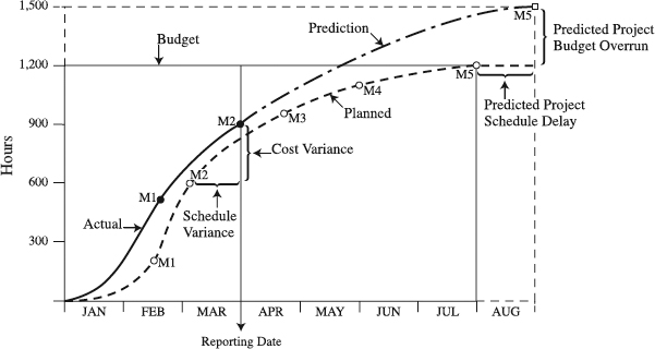
Figure 13.8 An example of Milestone Analysis.

Preparing these inputs, as described in the Earned Value Analysis section, is a prerequisite for the effective Milestone Analysis. Together, they form a bottom-up project baseline plan.

Set Up and Track Milestones. Using the Cost Baseline (Time-phased Budget), draw a planned cost performance curve that will be the baseline, annotating milestones on it (see Figure 13.8). This is a cumulative curve, typically expressed in resource hours or monetary units. A certain number of hours is budgeted for each milestone, and because of the cumulative nature of the curve, when a milestone is reached, the cumulative number of hours for the milestone and all preceding milestones should be consumed. As the project unfolds, actual cost data are collected and used to draw a cumulative actual cost curve, but what really matters is when a milestone is accomplished and marked on the actual curve. Hence, all performance is measured on the milestone level, following a fixed formula of 0/100, an approach of EVA: When the work on a milestone is started, 0 percent of the milestone's budget is earned, while the completion of the milestone earns a full 100 percent. Because of the cumulative nature of curves, the milestone acts as the culmination point of all previous project work, making its performance equate with project performance at that point.

Evaluate Project Results. This is the time to compare the actual results of performing the project against its plan. The goal is to establish the schedule variance (SV) and cost variance (CV), and to identify the cause of the variances, if any. A good way to prepare is to do a rehearsal with milestone owners, and then to implement the evaluation in a progress meeting (for details see the “Milestone Prediction Chart” section in Chapter 12). For both the rehearsal and meeting, an effective framework is the Proactive Cycle of Project Control (see the box that follows, “Five Questions for PCPC for Cost Control”).

In our example from Figure 13.8 the variances are as follows:

Schedule Variance for Milestone 2 = Planned − Actual = 2 months − 3 months = − 1 month

Cost Variance for Milestone 2 = Planned − Actual = 600 hours − 900 hours = − 300 hours

While the negative variance indicates that the project falls behind its plan, the positive variance means the project is ahead of its plan. No variance implies the performance is right on plan. Therefore, in our example, the project is one month late and 300 hours over the budget.

Predict Final Results. Certainly the most important and also the toughest step is the prediction of the final results. It is important because it enables a proactive look at the direction and trend of the project—where are our final cost and completion date going to end up? The absence of formulas for prediction such as those used in EVA makes the prediction an intuitive, challenging assignment, typically performed in the progress meeting. Such an exercise is very similar to one described in detail in the “Milestone Prediction Chart” section in Chapter 12. In particular, as the owner of the milestone describes its actual progress, potential variance from the baseline, and issues causing the variance, owners of dependent milestones opine the ripple effect of the milestone on subsequent milestones. The ripple effect is analyzed in the context of the critical path schedule, indicating the dependencies between milestones and related tasks. As a result of the analysis, predictions of milestones' cost and completion dates are made, all the way to the end of the project. If the final results are not favorable, corrective actions are charted to alter the trend and send the project back on track.

Utilizing the Milestone Analysis

When to Use. Milestone Analysis is a good candidate for both smaller and larger projects. With its visual power and little time to develop, the analysis serves well the needs of projects with smaller budgets. In larger projects, its primary rationale for use is its ability to supply summary view of the project status to high-level managers, focusing on high-level milestones.

Time to Use. With a bottom-up project plan already in place, a wellversed project team should take no longer than 30 to 45 minutes to perform a Milestone Analysis that includes five or six milestones. As the number of milestones increases, so will the necessary time for the analysis.

Benefits. Crucial to the benefits of the Milestone Analysis is an understanding that it is a simplification of EVA. Using a milestone as a precisely defined scope of work, the analysis integrates cost and schedule with the scope, eliminating the need for the earned value curve. As a result, the Milestone Analysis includes only two curves, as opposed to EVA's three. This makes it more attractive and easier to use than EVA, while providing some of the values created by EVA. In particular, Milestone Analysis establishes cost and schedule position, indicates performance trend and detects early-warning signals, integrates scope, cost, and schedule, and facilitates management by exception. Most often, these benefits are confined to smaller projects and larger projects that use the Milestone Analysis for higher-level milestones, its typical application areas. Since the Milestone Analysis with a large number of milestones tends to be convoluted and impractical, the analysis cannot be a single control system for all management levels in all projects, something that EVA is.

Advantages and Disadvantages. Two major advantages of the Milestone Analysis stand out:

• Graphic appeal. The ease of visually discerning the schedule and cost variances, along with the predicted line of future milestone performance, are bound to win the acceptance of mangers searching for a graphically appealing view of the project's summary status.
• Simplicity. Adding to the graphical appeal is the analysis' simplicity, enabling almost any project participants to grasp its message in several minutes of training.

Users should be aware of the Milestone Analysis's major disadvantages such as:

• Potential for confusion. When the analysis includes a large number of milestones, performing it may be confusing and challenging, although some companies experienced in its use apply it with hundreds of milestones.
• Potential for misuse. Some organizational cultures may misuse the cost and schedule variances, as well as final results predictions, primarily for performance evaluation of the project team. This may prompt teams to manipulate data in the analysis.

Variations. In the high-tech industry competing in the time-to-market race, there is a popular variation leaving out the cost variance and prediction. Consequently, the analysis is entirely focused on the schedule part, precisely the schedule variance and prediction of the final completion date of the project.

Customize the Milestone Analysis. The generic type of the Milestone Analysis may very well fit your projects. It is more likely, however, that certain adaptations could be made to better reflect your specific project situation. Following are a few examples to illustrate our point.

Customization Action	Examples of Customization Actions
Define limits of use.	Use the Milestone Analysis for all smaller projects.
	Use the Milestone Analysis only for milestones on the summary level of larger projects.
	Include no more than six-seven milestones in the analysis.
Amend an existing feature.	Use a formula for predicting the final project cost. For example, the final project cost = cumulative actual cost for the milestone + (project budget − cumulative actual cost for the milestone)/(cumulative plan cost for the milestone/cumulative actual cost for the milestone). These predictions could be made each time a milestone is achieved.

Summary

This section was about Milestone Analysis, a simplification of EVA. When a milestone is used as a precisely defined scope of work, the analysis integrates cost and schedule with the scope, eliminating the need for the earned value curve. As a result, the Milestone Analysis includes only two curves as opposed to EVA's three. It also indicates performance trend and detects early-warning signals equally well in smaller and larger projects. The following box presents the key points about performing the Milestone Analysis.

Concluding Remarks

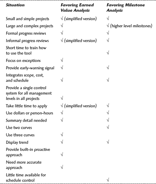
There are only two tools in this chapter: the Earned Value Analysis (EVA) and the Milestone Analysis. Both offer functionalities targeting certain applications. Still, project managers living under time pressures often ask, “Given my project situation, which one is more appropriate to use?” To decide, take a look at the set of project situations given in the following table, indicating how each situation favors the use of the two tools. First, identify the situations that correspond to your project. If these situations do not characterize the project well, think of more situations in addition to those listed, marking how each favors the tools. The tool with the higher number of marks for identified situations is probably a better fit for you (probably, because simplified versions of EVA may be an excellent choice in situations favoring either the Milestone Analysis or full-scale EVA). In any case, you should focus on a proactive method.

A Summary Comparison of Cost Control Tools

References

1. Fleming, Q. W. and J. M. Koppelman. 2000. Earned Value Project Management. 2d ed., Newton Square, Pa.: Project Management Institute.

2. Brandon, D. M. 1998. “Implementing Earned Value Easily and Effectively.” Project Management Journal 29(2): 11–18.

3. Fleming, Q.W. and J. M. Koppelman. 2001. “Earned Value for the Masses.” PM Network. 16(7): 29–32.

4. Dinsmore, P. C. 1999. Winning in Business with Enterprise Project Management. New York: AMACOM.

5. Hatfield, M. A. 1996. “The Case for Earned Value.” PM Network. 10(12): 25–27.

6. Barr, Z. 1996. “Earned Value Analysis: A Case Study.” PM Network 10(12): 31–37.

7. Harrison, F. L. 1983. Advanced Project Management. Hunts, U.K.: Gower Publishing Company.

8. Singletary, N. 1996. “What's the Value of Earned Value?” PM Network 10(12): 28–30.

9. Zwikael, O., S. Globerson, and T. Raz. 2000. “Evaluation of Models for Forecasting the Final Cost of a Project.” Project Management Journal 31(1): 53–57.

10. Christensen, D.S. and S.R. Heise. 1993. “Cost Performance Index Stability.” National Contract Management Association Journal. Vol. 25.

11. Beach, C.P. 1990. “A-12 Administrative Inquiry.” Navy Memorandum.

12. Lock, D. 1990. Project Planner. Hunts, U.K.: Gower Publishing Company.

13. Ingram, T. 1996. “Client/Server, Imaging and Earned Value: A Success Story.” PM Network 10(12): 21–25.