9

Risk Planning

Major topics in this chapter are risk planning tools:

• Risk Response Plan
• Monte Carlo Analysis
• Decision Tree

These tools are instrumental in identifying risks to the project, assessing their potential impact, and developing actions to mitigate them (see Figure 9.1). The preparation of such a risk baseline requires two-way exchange of information with scope, cost, and schedule baselines. Also important in this process is the coordination with other tools of organizational, quality, and procurement planning. During the implementation phase, the fortune of risk control will start off and be measured against the risk baseline. In a nutshell, risk planning tools create a strategy to fend off undesired events in projects.

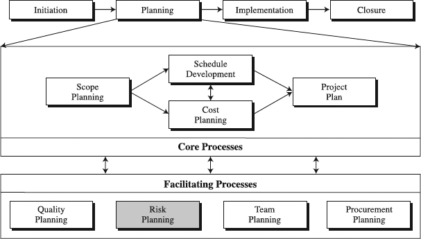
Figure 9.1 The role of risk planning tools in the standardized project management process.

The purpose of this chapter is to support practicing and prospective project managers in their quest to

• Learn how to use various risk planning tools
• Pick risk planning tools that are most appropriate for their project situation
• Customize the tools of their choice

Internalizing these skills plays a central role in project planning and building the standardized PM process.

Risk Response Plan

What Is the Risk Response Plan?

The Risk Response Plan assesses risks and identifies actions to increase opportunities and reduce threats to project goals [3]. To be effective, the plan must be realistic (as to the severity of the risk), timely, cost-conscious, bought into by all involved players, and owned by the appropriate person. Perhaps more than anything else the plan must be proactive, developing actions ahead of the risk occurrence (see Figure 9.2). Instead of being viewed as having a complete control of events, it should be seen as an advanced preparation for possible adverse future events [1].

Developing the Response Plan

Making decisions is perhaps the toughest of jobs that project managers have to take on. That wouldn't be very challenging in a situation of total certainty, when all information that they need for decision making is already available and the outcomes of their decisions are also known. Project managers' life, however, is much more complex, and most of their decisions are made with incomplete information and uncertain outcomes. This is the realm of project risk management. Beyond it lies the region of total uncertainty, with complete absence of information, where nothing is known about outcomes. This total certainty (knowns)—risk (known unknowns)—total uncertainty (unknown unknowns) continuum is illustrated in Figure 9.3.

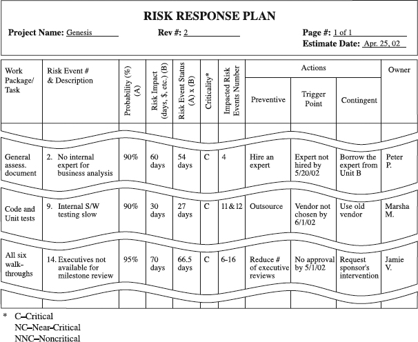
Figure 9.2 An example of the Risk Response Plan.

Figure 9.3 The uncertainty continuum and risk response planning.

From Project and Program Risk Management: A Guide to Managing Project Risks and Opportunities by R. Max Wideman. Copyright © 2000 by Project Management Institute. Reprinted with permission of Project Management Institute.

Our focus is on the risk area by developing a Risk Response Plan through a simple cycle of identify, assess, respond, and document. Basic definitions are included in the box that follows, “Basic Risk-Related Definitions.”

Prepare Information Inputs. An ideal in risk planning is to take it as rigorously as we take cost or schedule planning. In pursuit of such an ideal, you should start with rigorous inputs, including the following [5]:

• Risk management plan
• Project planning outputs
• Risk categories
• Historical information

The risk management plan is a document developed in the beginning of the project that provides a roadmap for dealing with risk throughout the project's life. Included into the plan may be the following [5]:

• Methodology. Identifies and describes approaches, tools, and data sources that may be used to handle risks.
• Roles and responsibilities. Define who does what in risk management in the project, from project team members to members of the company's risk management teams.
• Budgeting and timing. Specify the budget for risk management for the project, as well as the frequency of the risk management processes.
• Tools. Describe which specific methods for qualitative and quantitative risk analyses to use and when to use them
• Reporting and tracking. Defines the format of the Risk Response Plan and report, how the results of risk activities will be documented, communicated to stakeholders, and preserved for purposes of lessons learned.

Obviously, the purpose of the risk management plan is not to address individual risks in a project; rather, it is to guide a project team in developing a Risk Response Plan and then monitoring its performance.

Project planning outputs—performance baseline including scope, cost, time, and quality baselines—are what is at risk. Having full knowledge of them is crucial in developing response plans to counter risks to which the outputs will be exposed. These risks can be organized into different categories. For example, risks can be classified according to their effect on the project—scope, quality, schedule, and cost risks (in other words, failure to complete the project tasks within planned scope, quality, schedule, and cost performance). Another way is to categorize risks per their primary source into external (but unpredictable), external predictable (but uncertain), internal non-technical, technical, and legal [1]. This perspective looks for the balance between the internal and environmental impacts. The point is that the firm and its projects need a consistent risk categorization, suiting its business and culture, which can serve as a framework for a systematic identification and treatment of risks. Since risk management tends to be data-intensive, reliable historical information such as past project records, postmortems, or published sources (e.g., product benchmarking studies) is vital. Although it furnishes precious knowledge of what might go wrong, it is important to read past experience correctly when applying it in foreseeing risks to the current project.

Identify Risks. This step's purpose is to identify all the potential risks that may significantly influence the success of the project. Multiple ways for accomplishing this step are available, ranging from engaging the project team in a brainstorming session to consulting experienced team members to requesting opinions of experts not associated with the project. In any of them, several things have to be taken into account. First, risks vary across the project life cycle. Typically, risks tend to be relatively high early in the project because so many resources remain to be invested. Similarly, later in the project when most of resources are invested, most of unknowns are turned into knowns and risks are relatively lower. Also, some risks occur only in certain project stages; for example, risks related to project acceptance tests are typically encountered at the project end. Sometimes, even assumptions may become a source of risk (see the box that follows, “Is an Assumption a Risk?”). This dynamic nature of risks makes the identification process iterative, requiring that once risks are identified early in the project, they need to be continuously reviewed, with appropriate adjustments [6].

Second, risk events rarely strike independently. Rather, they tend to interact with other risk events, combining into larger risks. Looking for such interactive possibilities is important in risk identification. Finally, since risks come in all types of packages, planners should conduct risk identification in a systematic way so that no stone is left unturned internally in the project and externally in the environment, including management of stakeholders. A huge help in this respect may be received from risk categorization. For this purpose, our example in Figure 9.2 uses WBS as a systematic framework for risk identification (column 1). Beginning with the first work package, we may ask our project team, “What may go wrong?” meaning what risk events can hit our work package (column 2). Or, we can use any of the risk categorizations—formed according to the effect or primary source—as a checklist to identify possible risks for our first work package, and then continue similarly for all other work packages. Relying on WBS for this purpose also provides benefits such as cross-project consistency and comparison and creation of historical risk database.

Assess Qualitatively. A usual problem at this time of risk assessment is that a large number of risks might have been identified. Which ones deserve attention? Apparently, those that have both the highest impact on the project and are most likely to occur. While a preliminary clue is to look at the WBS to spot these critical risks—they are probably in most important portions of WBS—we still need to analyze impact, probability, and severity (criticality) of each risk.

In the qualitative assessment, we tend to use a nonnumeric probability scale—for example, a five-level scale, where 1=very unlikely, 2=low likelihood, 3=likely, 4=highly likely, and 5=near certain [7]. If you don't have much experience or data to reliably assess quantitative probabilities—addressed later in the quantitative assessment—nonnumeric scales are sufficiently good. Consequently, you will qualitatively assess each risk's probability on this nonnumeric scale. When this is done, the next step is to assess the impact of each risk, again on a discrete scale. One example is a scale such as 1=very low impact, 2=low impact, 3=medium impact, 4=high impact, and 5=very high impact. To illustrate its use, let's assume that a risk to be assessed has three impacts: project costs can increase, schedule can slip, and quality can be reduced. For each one of them, the scale can define the levels of impact, as shown for the schedule risks in Table 9.1. After each of the three impacts is rated, the overall impact rating of the risk is the largest of the three impacts [8].

When all risks are assessed like this, it is time to use a formula to combine their risk probability and impact to establish a measure of severity. Although nonlinear formulas can be employed, linear formulas such as Severity = Probability + N x Impact are easier to apply. For example, N can be equal to 2, meaning that impact is twice as important as probability in establishing risk severity. In this case, the assessed probability and impact for each risk would be entered in the formula Severity = Probability + 2 x Impact and the obtained value input into the Probability-Impact (P-I) matrix consisting of 5 × 5 squares (see Figure 9.4). The matrix is usually divided into red, yellow, and green zones, representing high severity (critical—first priority), medium severity (near-critical—second priority), and low severity (noncritical—lower-priority) risks, respectively, based on the organization's thresholds for risk severity. If you have a large number of risks, the position of a risk in the matrix determines its ranking and, thus, severity. squares with the highest values have the highest ranks, and squares with equal value may be ranked in order of their impact level [8]. Still, a question remains: How many of the highest-ranking risks should we deal with?

Some larger projects commonly focus on the top ten highest-ranked risks. In contrast, some smaller projects decide to manage the top three risks, arguing the lack of resources to take on a larger number of risks. Both may be dangerous. If these projects have more than ten and more than three risks in their red zone, respectively, they are bound to disregard some critical risks. On the other hand, if both of them are facing only one risk in their red zone, and others are in the green zone, they are wasting their resources looking at the top ten and three risks.

Table 9.1: Example of Rating a Risk Impact on Schedule on a Five-Level Scale

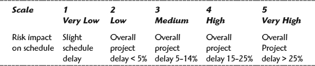
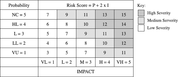
Figure 9.4 Segregation of risks into low, medium, and high severity by Probability-Impact matrix.

So, what is a reasonable way out? The answer is in the P-I matrix. Respond to the highest-ranked risks in the matrix, down to an agreed level [8]. For example, focus on handling risks down to risk score 11 (see Figure 9.4), and treat other risks as noncritical. With this approach, you neither squander resources nor disregard significant risks.

As mentioned earlier, if you don't have much experience or data to reliably assess quantitative probabilities, qualitative assessment of risks based on nonnumeric scales is good enough. They should proceed to the respond step. For those with experience and reliable data, the next action is quantitative risk assessment.

Assess Quantitatively. This step analyzes numerically the probability of each risk, its consequences on project objectives, and the extent of overall project risk [5]. It can be used separately or together with qualitative assessment. For example, if the available time and budget permit, and both qualitative and quantitative analysis are desired, the “together” approach may be the clear choice. This is our choice here as well.

The process begins from the results of the earlier risk identification step. For each of these identified risks, you need to quantify the probability of occurrence by asking, “What is the probability that this risk will happen?” “Ninety percent,” the team decides. This means that there is a 10 percent probability that the risk will not occur. Clearly, the probability that the risk will occur plus the probability that it will not occur equals 1. Assessing the probability is no more than an estimate based on solid historical information from similar experiences in past projects or considerate opinion of experts. In our example from Figure 9.2 (risk event 2, column 3), the team reviewed past records and solicited inputs from several experienced project mangers. On that basis, each team member developed an estimate of probability, and after a team discussion, a consensual number of 90 percent was adopted.

The next step is to determine the risk impact. “What is the severity of consequences if this risk occurs?” is the question you should ask. While the impact may be expressed in almost any units, from percent of lost market share to customer fallout percent, the real emphasis here is to estimate schedule or cost severity of the risk. In our example, the project's goal is all about delivering on schedule; therefore, the impact focuses on schedule (Figure 9.2, column 4). With this data, the risk event status (also called criterion value or ranking) can be determined by the following relationship [1]:

In our example (Figure 9.2, risk event 2, column 5), this relationship gives the risk event a status of 54 days. When the status is calculated for all risk events, the natural question is which of them are really vital and deserve attention and which are trivial. To answer this question, we will use principles similar to those on the issue of severity in qualitative assessment. First, establish numerical intervals of severity that determine whether a risk event status is critical (potential showstoppers), near-critical (soon to be potential showstoppers), or noncritical (minor risks). For example, in a smaller project the risk event status exceeding 15 days was critical, between 7 and 14 days near-critical, and below 7 days noncritical. Second, respond to the highest-ranked risks, down to an agreed level. In an instance this meant focusing on the top ten risks only.

Right after you have determined the risk impact, a question emerges: “Does this risk event impact any other risk event?” If such is the case, identify the impacted risk events. The rationale here is that many smaller risks may interact, snowballing into a risk impact that significantly exceeds the sum of the individual risk impacts. To preempt such a possibility, the information about impacted risks will be used in the next step to define response actions.

Respond. The whole Risk Response Plan culminates into its most creative part—determining the proactive response actions from a range of possible responses to a risk event in order to reduce threats to the project. Such an action should be rooted in risk policies and procedures established in the risk management plan. In particular, a proactive response action includes three steps of implementation: preventive action, trigger point, and contingent action (see Figure 9.2, columns 8, 9, and 10). The preventive action is the primary strategy, or plan A, of responding to a risk. When executed, however, it may or may not work. The point at which we establish that the primary strategy doesn't work is the trigger point. At that time, the backup strategy or contingent action (plan B) is taken to counter the risk. For example, the preventive action for risk event 9 in Figure 9.2 is outsourcing software quality testing from a larger and well-staffed firm. If by June 1 the vendor to provide the testing is not selected and the purchase order issued, the preventive action is not successful and should be suspended. That's the trigger point at which we introduce the contingent action by going to our old vendor, which although not large, still has time to get the testing done.

Any suitable proactive response action essentially falls into one of the four broad categories of response strategies: avoidance, transference, mitigation, and acceptance of risk [5]. Changing the project plan or condition to eliminate the selected risk event is risk avoidance. When faced with the risk of not having an available expert to perform quality business analysis, the risk was avoided by hiring such an expert (see row 1 in Figure 9.2). Risk transfer simply involves shifting consequences of a risk event to a third party, along with the ownership of the response [5]. This means that a project exposed to a risk of slow software quality testing internally can transfer the risk by hiring a professional firm to do the testing (see row 2 in Figure 9.2). Mitigation's intent is to lower the probability or impact (or both) of an unfavorable risk event to an acceptable threshold. In our example in Figure 9.2 (row 3), the risk of busy executives slowing down the project is reduced by reducing the number of major milestone reviews they have to attend and approve/disapprove the continuation of the project. The three response strategies—avoidance, transference, and mitigation—are deployed when risks they are responding to are among the highest-ranked risks. Obviously, these responses will be incorporated in the project plan.

For those risks that are not among the highest-ranked risks, a risk acceptance strategy is used. It implies that project managers have decided to not change the project plan or are unable to articulate a feasible response action to deal with a risk [5]. A typical example of the risk acceptance is the establishment of contingency allowances. For an explanation of how the allowances are formed, see the box on page 296, “How Much Reserves and Allowances to Plan For?”

An integral part of the response development is the identification and assignment of risk owners—individuals or parties responsible for each preventive action, trigger point, and contingent action. In so doing, one should recognize that while some risks are independent, leaving their owners fully responsible for their management, some risks might be interdependent. If so, their preventive actions, trigger points, and contingent actions should be developed and owned interdependently.

Document. Summarizing the results of the risk response planning into a document with conclusions and recommendations allows managers to take several important actions [1]. To begin with, they can make project decisions fully recognizing the involved risks. Also, they can continue to evaluate risks on the current project. Finally, this document will serve as a baseline for risk management analysis in performing a postmortem review, a great source of information for historical risk databases. For example, one manufacturing company requires that risk assessments are archived with other project documentation in the Web site, shared drive, and project blue book (documents retained after the project completion, post-project project file).

Utilizing a Risk Response Plan

When to Apply. There is no project that cannot benefit from developing the plan. Small projects typically rely on the qualitative assessment and P-I matrix, often deciding to handle only a few highest-ranked risk events. Not surprisingly, the dominant mode of their planning is informal, as is the periodic reevaluation of the plan throughout the project. Although at times it may be overly simplistic for large and complex projects, the Risk Response Plan is nevertheless widely used, with more formality and stronger orientation on quantitative assessment. Focused on the larger number of highest-ranked risk events, larger projects also tend to do more formal, periodic reassessments of the plan.

Time to Complete. Lots of teams running small and simple projects are able and can afford to expend one to a few hours of their time to conduct a session and develop the plan. This time proportionately rises as projects get bigger and more complex. Tens of hours may be necessary for a team in charge of a large and complex project to devise a Risk Response Plan of this type.

Benefits. The Risk Response Plan helps sift through the myriad of uncertainties, pinpoint and highlight the project areas of highest risk, both before work has begun and throughout the project [9]. This offers you an opportunity to identify effective ways of reducing those risks in a proactive manner, rather than being confronted by them. Resulting from such opportunity is a benefit of incorporating risks directly in the process of planning and executing a project. This further enables better understanding of the project goals, scope, and feasibility [1]. In addition, the plan generates information for a more realistic project plan and implementation, a more reasonable contingency planning, and an early warning of risk.

Advantages and Disadvantages. The plan's major advantage is its

• Simplicity. This is especially true of the qualitative portion with its easy-to-discern color messages of severity levels. Rid of advanced statistics, its quantitative part is still simple and adequate for many projects.

But this simplicity also results in a major disadvantage:

• Individual focus. The plan's major focus is on individual risk events, and although it recognizes the risk of interacting risk events, it does not provide a reliable mechanism to deal with them. When its reliance on single-point estimates for probability and risk impact are added, it becomes apparent why critics suggest that if the plan is used in larger projects, it should not be used alone but in conjunction with other, more complex tools, Monte Carlo simulation, for example.

Variations. Variations of the P-I matrix and Risk Response Plan abound. The matrix goes by such other names as risk matrix [8] and P-I table, for example, while risk register is often used as a synonym for the plan [4]. These variations typically have different scales for the assessment of the probability and risk impact, formulas for the establishment of the measure of severity, and methods for the division of the matrix into severity zones. One such difference that is used in the P-I matrix enables ranking risks that have multiple impacts—schedule, cost, and quality, for example. When a single risk is identified, each of its multiple impacts is rated on the probability and impact similarly to the method from Table 9.1. The rating for schedule impact, for example, is used to determine a weighting for its probability (Wsp) and impact (Wsi). When this is repeated for cost and quality impact, the overall risk rating is (Wsp x Wsi) + (Wcp x Wci) + (Wqp x Wqi). These scores are then used for risk ranking. Vose refers to this approach as semiquantitative [4]. Similar approaches can be used for the calculation of risk event status and risk ranking in the risk response plan.

Customization Action	Examples of Customization Actions
Define limits of use	Make the plan's use informal in small projects, focusing on the top five risks.
	Make the plan's use formal in large projects, focusing on the highest-ranked risks, down to an agreed level.
Adapt a feature.	Adapt P-I matrix zoning to the company's thresholds of risk.
Add a feature.	Add semiquantitative approach to the P-I matrix.
	Add the time line for preventive/contingent actions.

Customize the Plan. As a generic tool, the Risk Response Plan may help a company to a certain extent. To derive more value from it will require adapting it to the company's specifics and projects. In the following we offer several ideas on how to go about the customization.

Summary

In this section we presented the Risk Response Plan, a tool that assesses risks and identifies actions to increase opportunities and reduce threats to project goals. Each project can benefit from developing the plan. Small projects typically rely on the informal, qualitative assessment, often deciding to handle only a few highest-ranked risk events. Focused on the larger number of highest-ranked risk events, larger projects also tend to do more formal, periodic reassessments of the plan. In this manner, the plan helps pinpoint and highlight the project areas of highest risk and identify effective ways of reducing those risks in a proactive manner. It also enables more reasonable contingency planning and an early warning of risk. In short, here are the key points in structuring the Risk Response Plan.

Monte Carlo Analysis

Monte Carlo Analysis (MCA) uses a model of a project—project network diagram, for example—to analyze its behavior. For this purpose, MCA randomly samples probability distribution of each project activity to “perform” the project hundreds or even thousands of times [5]. This provides statistical distribution of the calculated project durations and approximates the expected value of the project duration, as illustrated in Figure 9.5. With these distributions, you can quantify the risk of various schedule scenarios, alternative implementation strategies, activity paths, or even individual activities. For example, as Figure 9.5 indicates, there is a 40 percent probability that the project will be finished before or on May 20.

Performing Monte Carlo Analysis

Typically, MCA deals with schedule, cost, and cash flow risks, although other facets such as the quality of the final project product can at times be analyzed. Taken overall, performing a schedule risk analysis is more complex than a cost analysis, simply because you need to establish dependencies between project activities in order to identify the critical path. For this reason, our focus is on looking at the MCA process in schedule risk analysis (see Figure 9.6).

Prepare Information Inputs. Four inputs play a key role in MCA:

• Risk management plan
• Risk Response Plan
• Project logic diagram or schedule
• Probability distributions

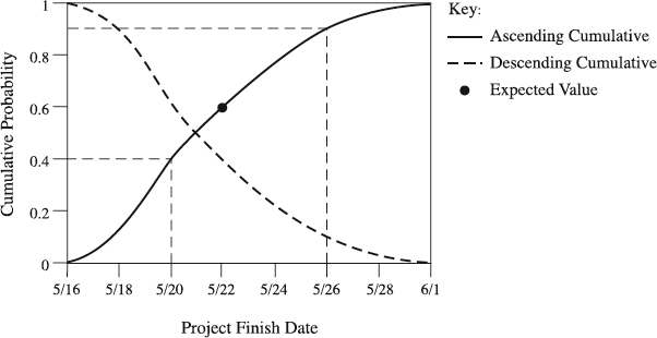
Figure 9.5 Cumulative distribution of project duration produced in Monte Carlo Analysis.

From Risk Analysis: A Quantitative Guide by David Vose. Copyright © 2000 by John Wiley & Sons Limited. Reprinted with permission of John Wiley & Sons.

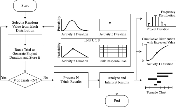
Figure 9.6 Process of Monte Carlo Analysis for schedule risk.

Since a risk management plan provides a roadmap for dealing with risk throughout the project's life, it is logical to expect it to offer directions for how to use MCA in the project. Another type of directions is contained in the Risk Response Plan. There, in particular, individual risks are identified, described, and analyzed to assess, rank (P-I matrix), and quantify them, along with preventive and contingent response strategies. All of this information will be fed into MCA to generate a range of possible project durations (see the box that follows, “Basic Language of Monte Carlo Analysis”). For that purpose, we also need the project network diagram that sequences project activities while indicating dependencies between the activities. Some prefer to start with the deterministic project schedule instead of the diagram, for example, formatting the schedule as the time-scaled arrow diagram, the cascade type (see Figure 9.7). Using the CPM schedule is also a valid option.

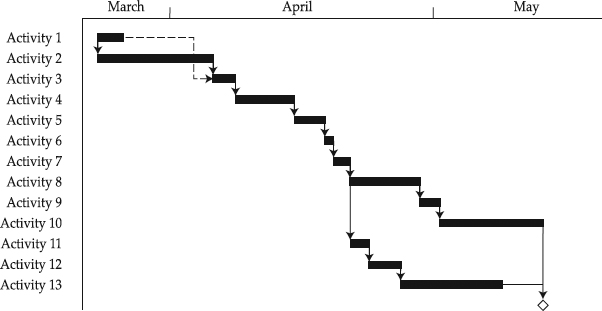
Figure 9.7 An example of the Time-scaled Arrow Diagram for risk analysis with Monte Carlo.

Generating a range of possible project durations and their probabilities is not possible without preparing probability distributions for project activity durations. This preparation process may begin with the question “How long does it take to complete a project activity?” Let's assume that you performed this activity many times and each time it took ten days to get it done. If asked to estimate the duration of that same activity in a future project, you would likely put it at ten days. If each project activity would have such a single point estimate (also called single value estimate) as an input to calculate project schedule duration, the duration would also have only one value. There is not much uncertainty in project activity durations in this single-valued deterministic model—they are all fixed. In the majority of today's projects, such a scenario is not realistic. More realistic is the following probabilistic (stochastic) model.

Imagine that you repeated activity 1 an extremely large number of times (trials, iterations, scenarios) and its duration ran from 5 to 39 days (range of outcomes). You recorded the fraction of times that each duration value (outcome) occurred. The fraction for a particular outcome is approximately equal to its probability (p) of occurrence for Activity l. When we have these approximate probabilities (the more trials you do, the closer the fraction becomes to the true probability) for all possible outcomes, we can chart them as probability distributions (see the activity 1 duration curve in Figure 9.6). Assume that experience-based probability distributions are also available for some other activities in the project as well (see activity 2 duration in Figure 9.6). If we really had such probability distributions (see the box that follows, “Frequently Used Probability Distributions”), they would be close to objective probabilities, which are defined as being determined from complete knowledge of the system and are not affected by personal beliefs.

Some activity durations, however, may be single-valued (e.g., activity n duration in Figure 9.6). Hence, we can have a combination of activity durations that are distributed and those that are single-valued. How does this impact project duration? As long as one or more activity durations (inputs to the model) are probability distributions, project durations (the outputs) will be probability distributions also [10].

Although some companies do have experience-based databases with the approximate distributions of their project activities, that is the exception rather than the rule. What, then, do we do to prepare probability distributions for activity durations? We will do what is a dominant practice in real-world projects—prepare and rely on subjective probabilities—someone's belief whether an outcome (activity duration) will occur.

The most adequate way for this is to enlist the help of experts, or experienced project participants. Brainstorming with activity owners, studying durations of similar activities in past projects, and consulting other specialists in the company who are not involved in the project all help determine the probability distributions or single values for the activity durations [4].

These distributions from past projects can be modified to reflect the information from Risk Response Plan mentioned earlier as a crucial input to MCA. For example, risk event status is determined for each individual risk event treated in the plan. If deemed appropriate by the project team, it is possible to expand the past-based distribution for the related activity to include the impact of the risk event status. In the case of the general distribution for a particular activity duration, that could mean increasing the maximum to reflect the risk event status. Updating the probability distributions with the information from the Risk Response Plan is the real way to determine the probability distributions most suited to each project activity based on the actual risks in the particular project.

Select Randomly a Value from Each Distribution. When the probability distributions are available for all project activities (variables), the stage is set for the next step. For each activity within its specific range of duration values, select one duration value randomly. The key word here is randomly. Using random sampling technique, MCA generates a random number between 0 and 1, which is fed into a mathematical equation that determines the activity duration value to be generated for the distribution [4]. All of these selected values constitute a random sample of values that will be used to generate project durations. Sampling can also be done with other efficient methods such as Latin hypercube sampling [4]. Whatever the method used, random sampling from probability distribution is performed in a manner that reproduces the distribution's shape [4].

Run a Trial to Generate Project Duration and Store It. Having a random sample of activity duration values means that for each activity in the project schedule there is one value only. Plugging this combination of activity duration values in the project network diagram will produce a scenario for project duration. In essence, this is a deterministic schedule with a single value for project duration, built on single-value durations for each activity. At this time, we will store this project duration until the time comes to use it again.

Repeating this sequence of random sampling many times and running a trial will produce as many scenarios for project duration, each one plausible. This prompts the question, “How many trials do we need?” Typically, trials (iterations) go until the predetermined number is reached (number N in the decision box in Figure 9.6). That number depends on the number of variables (activities) and the degree of confidence required but typically lies between 100 and 1000 [4]. The idea here is that sufficient number of trials preserves the characteristics of the original probability distributions for activities and approximates the solution distributions for project duration [10].

Process Results. When the trials are complete, our “storage” will contain N project durations. Each one is a possible case for the behavior of the project schedule. Processing them by means of a software program can produce many forms of results, whereas our focus is on the following (see the right-hand side of Figure 9.6):

• Expected value (EV) of the project duration. Averaging trial values for project durations approximates the expected value, the probability weighted average of all possible outcomes. However, the higher the number of trials, the higher the precision of the EV and the approximations of probability distribution shape for project durations.
• Frequency distribution. This is a histogram plot showing relative frequency obtained by grouping the data generated for project durations into a number of bars or classes. Frequency is the number of values in any class. Dividing the frequency by the total number of values will produce an approximate probability that the project duration (output variable) will lie in that class's range (see Figure 9.9).
• Cumulative frequency. It has two formats: ascending and descending (refer again to Figure 9.5). The former indicates the probability of the project duration being less or equal to the value on the x-axis. Conversely, the latter shows the probability of the project duration being greater than or equal to the value on the x-axis. Since the ascending format is more frequently used, we will stick with it. EV is marked on the plot with a black dot.

  

  Figure 9.9 Frequency distribution histogram of project duration.

• Tornado chart. This chart shows the extent to which the uncertainty of the individual activities' duration impacts the uncertainty of project schedule duration (see Figure 9.10). Specifically, the bar represents the degree of impact the activity (input variable) has on the project schedule (model's output). Therefore, the longer the bar, the greater the impact that the project activity has on the project duration. Per standard practice, bars are plotted from top down in decreasing degree of impact. When there are both the positive and negative impact, the chart is a bit reminiscent of a tornado, hence the name. To avoid the chart looking overly busy, Vose suggests limiting the plot to those activities (variables) that have an impact of at least a quarter of the maximum observed impact [4].

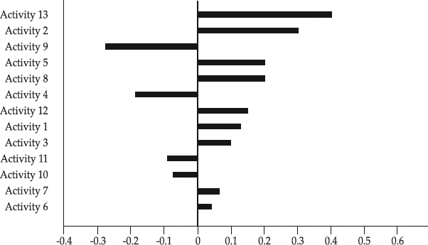
Figure 9.10 An example of the tornado chart.

From Risk Analysis: A Quantitative Guide by David Vose. Copyright © 2000 by John Wiley & Sons Limited. Reprinted with permission of John Wiley & Sons.

Analyze and Interpret Results. The results of the schedule risk analysis must be interpreted in a way that clearly provides answers to the questions the analysis was initiated to answer. For that reason, it is beneficial to follow four principles for schedule risk analysis [4]:

• Focus on the problem
• Keep statistics to a minimum
• Use graphs whenever appropriate
• Understand the model's (e.g., time-scaled arrow diagram chart) assumptions.

To demonstrate these principles, let's assume that the project team set out to perform the schedule risk analysis in order to answer these questions:

• How likely is it that the team will satisfy the project deadline (May 20) imposed by management?
• If the probability is lower than 90 percent (team's preferred probability), what do we do to negotiate the deadline with management?
• If we successfully negotiate the deadline issue, which are the top three activities in terms of their impact on project duration?

First, the team goes to the cumulative frequency graph (Figure 9.5). To obtain the answer to the first question, they will

• Enter the x-axis at the deadline date imposed by management (May 20).
• Move upward to the cumulative curve.
• Move left to the corresponding value on the y-axis. This y-axis value is the probability of completing their project before on the imposed deadline date (40 percent).

Clearly, the probability is very low, way lower than the preferred 90 percent. To answer the second question, the team decides to ask management for a new option of adding a contingency of six days to the imposed deadline, in which case the project would be finished by May 26 and would be 90 percent probable. To build a better case for negotiations with management, the team develops another new option. They combine the schedule crashing (throw in more resources in the project activities) and fast-tracking (overlap activities as much as possible) approaches. With this approach, they obtain the new project logic diagram and probability distributions for activities, and run MCA again. Going again through the cumulative frequency plot, they find out that the probability to meet the imposed deadline date of May 20 is 90 percent. Armed with the plot less redundant statistics, they approach management with both new options and successfully obtain new resource commitments from management for the second new option. Then, a look at the tornado chart (see Figure 9.10) reveals the three key activities with the highest impact on the deadline—these are top priorities to keep an eye on during the implementation, an answer to their question three. The team understands that their MCA is founded on (a) the changed logic of the time-scaled arrow diagram chart and (b) the changed probability distributions for activities that are based on new resource commitments. In a nutshell, the four principles for schedule risk analysis directed the team in its approach.

Utilizing Monte Carlo Analysis

When to Use. Traditionally, it has been the large and complex projects that have most often enjoyed the benefits of MCA. The belief was that, unlike smaller projects, larger projects had more important goals and could also afford necessary resources for performing MCA. It took some significant events for this view to start changing. First, the trend toward “management by projects” led to a proliferation of smaller but important projects. Also, very powerful desktop computer programs for MCA have become affordable. Finally, project offices capable of supporting many projects with MCA have become a frequent organizational unit. All of these events helped put MCA within the reach of smaller projects, changing the application pattern of MCA in corporations. Nowadays, MCA is used in both larger and smaller projects to respond to certain situations. For example, if the projects are sensitive to a completion deadline, MCA is a preferred option. Similarly, if there are many project scenarios and what-if analysis to explore, MCA is favored over decision trees [10]. When facing a situation where very small nuances may dictate which project wins the contest, for example, in the project selection process within the company, using MCA is the right move.

Time to Use. Roles in MCA crucially influence how much time it takes. A typical approach is to task the project office specialists or administrative assistants to perform MCA using the data provided by the project team. For a smaller project of 50 activities, for example, data entry and running MCA may take 10 to 30 minutes. Assuming that a project logic diagram exists, preparing activity probability distributions through team brain-storming and formatting them into a table to be fed to the project office may take an hour or two. The growing size and complexity of the project is bound to increase the time for MCA.

Benefits. Original project schedules and budgets are often unrealistic or, more precisely, inadequate. A major reason for this inadequacy is the uncertainty surrounding the project activities. In response to this uncertainty, many project teams assign an arbitrary duration or cost to the activities and hope for the best [8]. Contrast this approach with MCA, which allows richer, more detailed representation of the risk problem—important in some situations (see the box that follows, “Confident or Probable?”). Take, for example, a situation where a company's fortunes are at stake. If their new project does not develop a product to hit the market before their competitors, they may lose the market leadership. MCA would significantly improve quality of their decisions by offering a clear analysis of their risks, different scenarios, and probabilities of reaching the goal. Still in another situation, a project manager may be asked to finish a project by an unrealistic date or budget. To her, MCA provides the roadmap to lowering the risk by arguing against the unrealistic approach and obtaining resources necessary to complete the project as desired. In summary, MCA's value is in its ability to examine each project scenario, including the extreme scenarios, to see what conditions give rise to their results. That helps not only to validate the project realism but also to differentiate between what is possible and what is not possible, and most importantly, how to change what is not possible into what is possible [10].

Advantages and Disadvantages. MCA offers several advantages [4]:

• Basic mathematics. Mathematics needed to use MCA is quite basic. Even including complex mathematics or modeling correlation and other interdependencies (e.g., power functions, logs, IF statements, etc.) poses no extra difficulty.
• Easy to use. There are very good and commercially available software packages that automate the tasks involved in MCA. That means the computer does the work necessary to produce the outcome distribution.
• Easy to change. Making changes to the MCA model is a quick process that provides a great opportunity of comparing with previous models. Examining the behavior of each of the models is also straightforward.
• Legitimacy. MCA is seen as a well-reputed tool, increasing the likelihood that project teams and management will accept its results.

Often MCA is criticized for its disadvantages:

• Complex. Although based on basic mathematics, MCA is built on concepts of probability, a concept many project managers have yet to master.
• Approximate technique. Its outcome distributions are approximate, critics claim. While this is true when the number of iterations is small, you can easily overcome this problem by increasing the number of iterations until reaching the required level of precision.
• Takes time. There are complaints about the time a computer needs to generate iterations.

Customize the MCA. MCA is a risk analysis tool of great value that deserves to be used in the majority of projects facing an uncertain implementation environment. For that to be possible, the generic type of MCA that we have described has to be customized to fit the situation of an organization's projects. It is for that purpose that we offer several ideas for the customization.

Customization Action	Examples of Customization Actions
Define limits of use.	Use MCA in all projects taking over 1000 person-hours (major projects).
	Use MCA for risk analysis focusing on project schedule (in companies competing on time to market).
	Use MCA for risk analysis focusing on project cost (in companies competing on cost leadership).
	Use MCA focusing on Net Present Value when selecting new projects.
	Have project teams own the MCA, which will be performed by the project office (for organizations with a project office).
Adapt a feature.	Use the descending format of the cumulative frequency chart instead of the ascending format.
Add a feature.	MCA in larger projects must be accompanied by a risk analysis report including a model's assumptions, graphical representation of results, and conclusions, if any [4].
	Add spider and trend plots when the situation mandates so.

Summary

This section centered on Monte Carlo Analysis (MCA), a tool that uses a model of a project—a project network diagram, for example—to analyze its behavior and risks. The purpose is to lower the risk by arguing against the unrealistic approach and obtaining resources necessary to complete the project as desired. To accomplish this, MCA examines each project scenario, including the extreme scenarios, to see what conditions give rise to their results. That helps not only to validate the project realism but also to differentiate between what is possible and what is not possible. Still, it is the large and complex projects that enjoy these benefits of utilizing MCA. To recap the essence of this section, the box above offers the key points in performing the Monte Carlo Analysis.

Decision Tree

What Is the Decision Tree?

A Decision Tree is a graphical device for analyzing project situations under risk. Reflecting the decision process (see Figure 9.11), the tree displays sequential decisions in the form of the branches of a tree, from left to right, originating from an initial decision point and extending all the way to the end outcomes [11]. A path through the branches is composed of a sequence of separate decisions and chance events. The way to evaluate decisions is to calculate the expected value of each path, folding the tree back from the end points to the initial decision point [12]. For the description of a typical Decision Tree's components, see the box that follows, “Five Components of a Typical Decision Tree.”

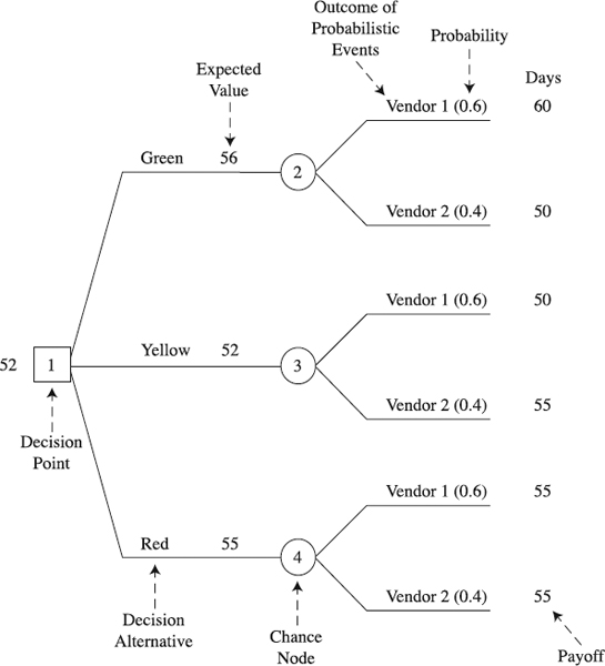
Figure 9.11 Decision Tree for a project situation under risk.

Analyzing the Decision Tree

Literature on Decision Trees often looks at minimizing the risk by selecting decision alternatives that offer maximum Net Present Value or minimum cost. The abundance of such examples prompted us to take a different approach. In particular, we look at the general process of analyzing Decision Trees on an example related to minimizing schedule duration. This is in response to risks faced by a large group of today's projects that must deliver the fastest possible schedule as an unconditional priority.

Prepare Information Inputs. Three major inputs have the central role in building and analyzing the Decision Tree:

• Risk management plan
• Risk Response Plan
• Other project information

As a roadmap for dealing with risk throughout the project's life, the risk management plan specifies how to use Decision Trees in project decisions under risks. Information contained in the Risk Response Plan about individual risks and their response strategies is also crucial. In our example from Figure 9.11, this information will be funneled into calculating durations for each of the outcomes in the Decision Tree. For these calculations, we also need other project information such as network diagrams of the decision alternatives for the central module design.

Describe Decision under Risk. Common sense dictates that in order to make the best decision, we first need to understand the decision context and related risks a project is facing. A convenient way for this is to describe the decision. Here is an example.

Fast Corporation competes on time-to-market capabilities. As they are entering the design phase for its new enterprise server development project, their goal is to finish it as soon as possible and hit the market before the competition. While literally each project day is considered to be of extreme priority, the development cost is given low importance. In such a situation, the project team is attempting to decide on the appropriate design approach to use for this product. A major uncertainty regards how many days it will take to design the central module in the product. Three major alternatives are being considered, each one identified with a single word:

• Green (G). Incorporate the routing rules early in the central module design.
• Yellow (Y). Predict the routing rules early and modify them at the end of the central module design.
• Red (R). Incorporate the routing rules at the end of the central module design.

The second uncertainty is related to an off-the-shelf part that goes into the central module, whichever the alternative. Two different vendors that cannot be influenced produce the part. It is well known that both companies are racing each other to put out the newest upgrade of the part in the market, and they have announced the same release date. To represent this decision description and enable its analysis, the team must first structure the model.

Structure the Model. The model is drawn from left to right (for a better understanding refer again to the “Five Components of a Typical Decision Tree” box). Therefore, draw a decision node (the square marked 1), then add to its right-hand side three branches, for three available design alternatives—the green, yellow, and red (Figure 9.11). Put a chance node (the circles marked 2, 3, and 4) at the end of each branch, followed by two branches, each one for outcomes of probabilistic events—vendor 1 hitting the marker first and vendor 2 hitting the market first. As monotonous as structuring the model appears, it is precious in sharpening our understanding. As a decision guru put it, these models help formalize common sense for decision models that are too complex for informal use of common sense [12].

Assess the Probability of the Possible Outcomes. Fast Corporation's server development project team cannot wait for the actual release of the first-to-market part by vendor 1 or vendor 2. That would significantly extend the module design schedule, jeopardizing the whole server project. Therefore, the project team decides to assess the probability of who—vendor 1 or vendor 2—will release the product first. Their research and past performance of the vendors led them to assess that there is 60 percent probability that vendor 1's part will first reach the market. The probability for the part from vendor 2 is 40 percent. Everybody on the team is clear that these are subjective probabilities influenced by their perceptions and beliefs. Adding the probabilities to the tree model is useful (see Figure 9.11).

Determine Payoffs of the Possible Outcomes. The project team has developed initial network schedules for each of the design options—green, yellow, and red—as if the vendor part is already available. Essentially, the sequence of design activities involved in each option is different, as well as some of the activities. Also, although both vendors' parts can be used for the central module, the process of their incorporation into the design options is different, causing the duration of each outcome to differ. Because the team's expectation is that the first-to-market vendor part will be released sometime midway through the module design, they need to evaluate how such a release is going to change the initial network schedules. The product of their evaluation is a set of possible outcomes values, also called payoffs. These schedule durations of the outcomes expressed in days are added at the end of each branch (see Figure 9.11).

There are two conceptually different parts to a Decision Tree analysis. Included in the first part are structuring the model, assessing the probabilities of possible outcomes, and their payoffs. This is a particularly unstructured task, requiring a significantly greater proportion of effort. The second part—evaluate alternatives and select the strategy—is the easy part of the model and the heart of the decision analysis under risk. We address it next.

Evaluate Alternatives and Select the Strategy. Our objective is to evaluate possible outcomes and design alternatives and select one with the shortest-possible schedule. To accomplish this, we need to solve the tree (see the box on page 314, “Two Simple Steps for Solving a Tree”). When these steps are applied:

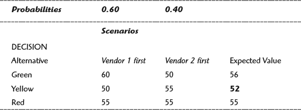
Step 1. Chance Node 2 EV (Expected Value): (0.60 × 60 days) + (0.40 × 50 days) = 56 days

Chance Node 3 EV (Expected Value): (0.60 × 50 days) + (0.40 × 55 days) = 52 days

Chance Node 4 EV (Expected Value): (0.60 × 55 days) + (0.40 × 55 days) = 55 days

Step 2. The best alternative is the alternative with lowest EV, the shortest schedule – 52 days. That means the team goes with the yellow option.

Decision Tree analysis enables more than just identifying the best alternatives. Sensitivity analysis, as well as tornado and spider charts, can also be developed to better understand the decision under risk [2]. They, however, are beyond our scope.

Utilizing Decision Trees

When to Use. Theoretically, we can use a Decision Tree to evaluate any decision under risk, regardless of its complexity, as long as the decision and probabilities of the possible outcomes are specified [12]. Practically, this is not the case. Rather, practicing project managers see the tree as a method to address daily problems, requiring a straightforward and quick selection of the best alternative. Why is this? The issue here is that complex decision situations lead to a “combinatorial explosion” and the time associated with it. As we add decision and chance nodes, the trees tend to grow exponentially [10]. For example, multiple alternatives with multiple uncertainties can explode Decision Trees into hundreds of paths, which is where Monte Carlo has a significant advantage. Constructing and solving for such trees may take hundreds of hours. Who can really afford this when our projects are in the fast lane? Perhaps only very large projects with generous budgets can do so. Since such are exceedingly rare, practicing project managers go to decision trees primarily when they need to swiftly evaluate simple alternatives, pick up the best, and go on with their daily routine [10]. Still, the majority of such situations occur in larger projects, although we have seen small project managers using two-alternative with four to six paths very informally with minimum time consumption.

Time to Use. Two extremes can help fathom the time requirements of Decision Trees. Spending 10 to 15 minutes to construct and evaluate a two-alternative Decision Tree with four paths seems realistic to many project managers. On the other hand, tens of hours may go into the construction of a Decision Tree with hundreds of paths. The assumption here is that information necessary to estimate probabilities and outcome values is already available. The analysis of large trees may be a matter of minutes, given the power of professional software necessary to use large trees. In case of smaller and medium projects Excel spreadsheet does a fine job.

Benefits. Two major benefits seem to motivate project managers to use Decision Trees. First, Decision Trees reduce an evaluation and a comparison of all decision alternatives under risk to a single value metric. Simply, this metric indicates the degree of support of project goals [10]. In our example, that metric was schedule calendar day, gauging progress toward Fast Corporation's quest for time-to-market speed. In other cases, an additional convenience stems from the fact that most of the time this single value metric is expressed in monetary terms, a universal language of business and projects. Then, this single monetary value combines cost, schedule, and performance criteria.

The second benefit lies in the belief of many project managers that the real value of Decision Trees is not in the numerical results but rather in their ability to help us gain insights into decision problems. With or without the numerical results, the users should understand that Decision Trees do not provide an entirely objective analysis. In the absence of sufficient empirical data necessary for a complete analysis, many facets of the analysis are rooted in personal judgment – structuring the model, assessing probabilities or payoffs, for example. Still, experience has shown that the Decision Tree tool is very beneficial [12].

Advantages and Disadvantages. Decision Trees are characterized by some advantages that are difficult to match:

• Convenience. Decision Trees are very convenient to visualize and analyze project decisions with one or a few paths. When more paths are added, the power of the trees is in their ability to augment our intuition.
• Visual impact. When seemingly intangible decision alternatives under risk are displayed in a Decision Tree format, they appear tangible for the tree's clarity and visual impact.

These should be weighed in against disadvantages such as:

• Low rate of use. Surprisingly, Decision Trees have not seen much use by practicing project managers. This is unfortunate because they offer value in risk deliberations that other tools cannot match, making us believe that in promoting this tool to project managers we should position it as a quick and informal tool for simpler decisions under risk.
• Complexity. Given how larger Decision Trees may become cumbersome and complex, it is understandable that they turn regular practicing project managers off. Application of such trees in projects should be the specialists' province of work.

Variations. A payoff table can easily represent very simple Decision Tree problems. Table 9.2, for example, is a tabular variation of the Decision Tree from Figure 9.11. It presents decision alternatives, probabilities of possible outcomes, payoffs, and expected values in a less visual format than the tree. Also, as the number of nodes and paths grow, the tabular format becomes increasingly difficult to use.

Customize the Decision Tree. The generic use of Decision Trees as described here will certainly provide value to the user. Customizing trees to fit one's projects' needs may further enhance the value. The following ideas may help you get a better feel for the customization.

Table 9.2: Tabular Representation of Decision Tree Problem in Figure 9.11

Customization Action	Examples of Customization Actions
Define limits of use.	Use Decision Trees with the help of professional decision analysts and professional software (large projects).
	Use small and simple Decision Trees either informally (e.g. on the back of an envelope) or with the help of Excel to quickly make decisions (small projects).
	Use the expected value (EV) schedule metric (time-to-market companies), EV cost metric (cost-conscious companies), or expected monetary value (EMV) metric as your company strategy mandates.
Adapt a feature.	Use a tabular format (if that's easier for project team members).

Summary

This section focused on the Decision Tree, a tool for analyzing project situations under risk. Decisions Trees can be used in both large and small projects. Practicing project managers see the tree as a method to address daily problems, requiring a straightforward and quick selection of the best alternative. A major benefit of the trees is in reducing an evaluation and a comparison of all decision alternatives under risk to a single value metric. Also, the trees help us gain insights into decision problems. In summary, these are the key points in performing the Decision Tree analysis.

Concluding Remarks

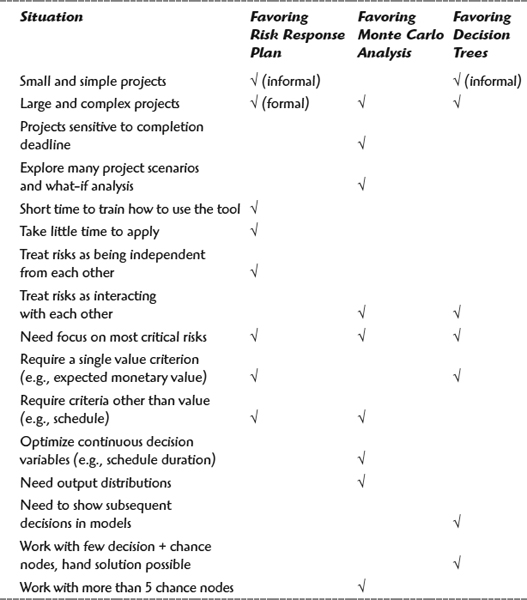
Two aspects are crucial in selecting when to use the Risk Response Plan, Monte Carlo Analysis, and Decision Trees. First, a Risk Response Plan is a convenient choice for treatment of risk events that are assumed to be independent of each other (which may not be the case), whether in small or large projects, formally or informally. Its highest value is when applied in conjunction with Monte Carlo Analysis or Decision Trees, as complementary tools, because the latter two are able to account for interacting risks. Second, Monte Carlo and Decision Trees are often seen as alternatives. So, which one is more appropriate to use? Of course, it depends on the project situation. Review project situations in the table that follows to understand how each one favors the use of the two tools, and select those that match yours. If necessary, identify more situations in addition to those listed and mark how each favors the tools. The tool that has the higher number of marks is probably a better choice for your project.

A Summary Comparison of Risk Planning Tools

References

1. Wideman, M. 1992. Project and Program Risk Management. Newton square, Pa.: Project Management Institute.

2. Winston, W. L. and W. S. Albright. 2001. Practical Management Science. 2d ed. Pacific Grove, Ca.: Duxbury.

3. Royer, P. S. 2000. “Rock Management: The Undiscovered Dimension of Project Management.” Project Management Journal 31(1): 6–13.

4. Vose, D. 2000. Risk Analysis: A Quantitative Guide. 2d ed. New York: John Wiley & Sons.

5. Project Management Institute. 2000. A Guide to The Project Management Body of Knowledge. Drexell Hill, Pa.: Project Management Institute.

6. Couillard, J. 1995. “The Role of Project Risk in Determining Project Management Approach.” Project Management Journal 26(4): 3–15.

7. Graves, R. 2001. “Open and Closed: The Monte Carlo Model.” PM Network 15(2): 48–52.

8. Graves, R. 2000. “Qualitative Risk Assessment.” PM Network 14(10): 61–66.

9. Hulett, D. T. 1995. “Project Schedule Risk Assessment.” Project Management Journal 26(1): 21–31.

10. Schuyler, J. 2001. Risk and Decision Analysis in Projects. 2d ed. Newton square, Pa.: Project Management Institute.

11. Cleland, D. I. and D. F. Kocaoglu. 1983. Engineering Management. New York: McGraw-Hill.

12. Eppen, G.D., et al. 1998. Introductory Management Science. 5th ed. Upper Saddle, N.J.: Prentice Hall.