
2
Project Selection
This chapter is contributed by Dr. Joseph P. Martino.
In research the horizon recedes as we advance, … and research is always incomplete.
Mark Pattison, Isaac Casaubon
True as these words may be, managers still need to make choice among possible projects, and either see them through to completion or terminate them when they “turn sour.” This chapter is intended to help managers use the following tools to select project that have a good chance of succeeding and paying off:
- Scoring Models
- Analytic Hierarchy Process
- Economic Methods (Payback Time, Net Present Value, Internal Rate of Return)
- Portfolio Selection
- Real Options Approach
These tools are designed to select projects that maximize the value of project portfolio for the company and are aligned with its business strategy. The assumption is that you have more candidate projects than you can support with available resources. To help you select from your project menu, this chapter provides a collection of tools that account for financial, technical, behavioral, and strategic criteria or factors in evaluating and selecting projects. The project mix will be in a state of constant flux, as management reevaluates its selections on an ongoing basis to respond to changing competitive and other needs. Project selection tools allow management to select projects for initiation and termination as conditions change.
The goal of this chapter is to help practicing and prospective project managers and managers accomplish the following:
- Learn how to use various project selection tools.
- Select project selection tools that match their project situation.
- Customize the tools of their choice.
Mastering these skills has a central role in initiating projects and building the SPM process. See Figure 2.1 for where these tools fit into the project management process.
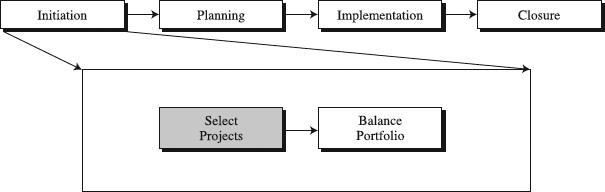
Figure 2.1 The role of project selection tools in the standardized project management process.
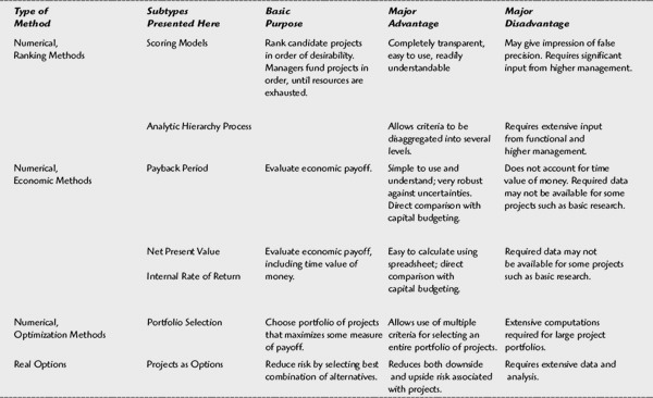
Table 2.1: A Comparison of Project Selection Methods
Scoring Models
What Are Scoring Models?
A Scoring Model includes a list of relevant criteria the decision maker wishes to take into account when selecting projects from the candidate menu. Projects are then rated by decision makers on each criterion, typically on a numerical scale with anchor phrases. Finally, multiplying these scores by weightings and adding them up across all criteria will produce a score that represents the merit of the project. Higher scores designate projects of higher merit. The Scoring Model can be designed specifically for any given selection situation. For better understanding of the position of the Scoring Models in the family of project selection methods, see Table 2.1.
Applying Scoring Models
Collect Information Inputs. Like other methods, Scoring Models follow the basic steps of project selection process (see box, “Basic Project Selection Process”). To be fully functional and meaningful, the models need a candidate project menu to choose from. In reality, what goes with the menu is a set of quality inputs including:
- Project proposal
- Strategic and tactical plans
- Historical information.
Since the purpose of the models is to help maximize the value of the selected portfolio of projects for the company, understanding which of the company's goals a project supports is a key point. While these goals are described in the strategic and tactical plans of the organizations, project proposals offer specifics on projects. To make better decisions, decision makers should also rely on the historical information about both the results of past project selection decisions and past project performance. When these inputs are available, you can move to choose relevant project selection criteria.
Select Relevant Criteria. One of the major reasons for the failure of the Scoring Models is constructing them on inappropriate criteria. Consequently, a key to Scoring Models appears to be in compiling an appropriate list of scoring criteria that well reflect the strategic financial, technical, and behavioral situation of the company. The challenge often seems to be in overcoming the temptation to develop a detailed and, therefore, cumbersome list of criteria that becomes unmanageable. Therefore, narrowing down to the vital few criteria that really matter is rather difficult, especially when the menu of criteria to start from is deceptively long. Consider, for example, criteria from the box coming up in the chapter titled “Criteria to Be Considered in Project Selection.” To be used effectively, most of them need to be broken into more specific items (see Table 2.2 for an example of the breakdown into 19 specific criteria). This further elevates the challenge of sticking with the vital few. That the challenge is real can be seen from experiences of some companies in which models fell in disuse because they included 50+ criteria. A smart approach used by some leading companies is in conceiving the list and refining over time with the intent to reduce the number of criteria.
Construct a Scoring Model. To construct a model, you must understand and resolve several issues:
- Form of the model, with certain categories of criteria or factors
- Value and importance of criteria
- Measurement of criteria
First we will deal with forming of the model. A “generic” scoring model would have the following form:
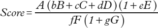
In this model, the symbols A, B, C, D, E, F, and G represent the criteria to be included in the score for the project. The value of each criterion for a given project is substituted in the formula. The symbols b, c, d, e, f, and g represent the weights assigned to each criterion. In the model, the criteria in the numerator are benefits, while the criteria in the denominator are costs or other disbenefits. The criteria are selected by management, as are the weights. The values of the criteria are project-specific and are normally provided by the project team.
Basic Project Selection Process
What types of projects are candidates (e.g., product development, market entry, capital projects, continuous improvement, etc.)? This question is addressed in the beginning step of the project selection process (see Figure 2.2). It creates the candidate project menu and is followed by selecting relevant criteria. The purpose is to include factors that help maximize the value of project portfolio for the company.
Figure 2.2 Basic project selection process.
Also known at this time should be the constraints such as budget, staffing, and so on. Important in this is to make sure that any policy considerations and strategic plans have been taken into account (e.g., support of existing products or construction of the new fab). The criteria will be plugged into the preferred selection tool to decide which projects from the candidate menu to choose for initiation or continuation.
Criteria to Be Considered in Project Selection
Criteria (or factors) that are relevant in project selection depend on the type of projects and their situation. For example, the following criteria are typically considered in choosing research and development projects. This list is intended to be suggestive rather than complete.
Although many of these criteria may be in selecting different types of the analysis whatever criteria are used projects, the important thing is to include in relevant to your project situation.
The model uses three categories of criteria:
- Overriding criteria (e.g., A). These are factors of such great importance that if they go to zero, the entire score should be zero. For instance, factors to be included in the model might be measures of performance such as efficiency or total output. A performance measure of zero should disqualify the project completely, regardless of any other “merit.”
- Tradable criteria (B, C, D, F). These are factors that can be traded against one another; a decrease in one is acceptable if accompanied by a sufficient increase in another. For instance, the designer may be willing to trade between reliability and maintainability, so long as “cost of ownership” remains constant. In this case, the weights would reflect the relative costs of increasing reliability and making maintenance easier. Cost F is shown as a single criterion that is relevant to all projects. Typically this would include monetary costs of the project. This might be disaggregated into cost categories such as wages, materials, facilities, and shipping, if there is the possibility of a trade-off among these cost categories (e.g., using a more expensive material to save labor costs). If no such trade-off exists, the costs should simply be summed and treated as a single factor.
- Optional criteria. These are factors that may not be relevant to all projects; if they are present, they should affect the score, but if they are absent, they should not affect the score. Note that either costs or benefits may involve optional factors. For instance, E in the formula represents a benefit that may not be a consideration with all projects. It should be counted in the score only if it is relevant to a project. For example, this might be a rating of ease of consumer use, which would not be relevant to a project aimed at an industrial process. G in the formula represents an “optional” cost that might not be relevant to all projects. Typically this type of cost is one in which the availability of some resource is a more important consideration than its monetary cost. For instance, there may be limits on the availability of a testing device, supercomputer, or a scarce skill such as a programmer. In such a case, the hours or other measure of use should be included separately from monetary cost and should apply only to those projects requiring that resource.
The second issue focuses on value and importance of criteria. Once the form of the model is selected, the designers of the model need to distinguish between the value of a criterion and the weight or importance of that criterion. In the preceding formula, B, C, and D are the values of their respective factors for a specific project, while b, c, and d are the weights assigned to those factors, reflecting the importance assigned to them by the decision maker. In the case of the tradable factors, the ratio b/c represents the trade-off relationship between factors B and C. If B is decreased by one unit, C must be increased by at least the amount b/c for the sum of the tradable factors to remain constant or increase. That is, the decision maker is willing to trade one factor for another according to the ratios of their weights, so long as the total sum remains constant or increases.
A very simple model used to score the project in Table 2.2 (see column item) is as follows:
![]()
Simply, the score is equal to the sum of B, C, and D, the values of their respective criteria such as “Unique Product Functionalities” or “Technical Complexity” (Table 2.2).
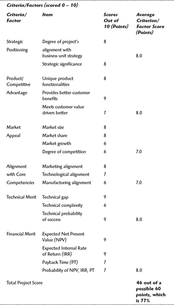
Finally, the third issue to resolve is one of measurement of criteria. Some criteria are objectively measurable, such as costs and revenues. Others, such as probability of success or strategic importance, must be obtained judgmentally. Scoring Models can readily include both objective and subjective or judgmental criteria. It is helpful if the judgmental criteria are estimated with a scale with anchor phrases, to obtain consistency in estimating the magnitude of the factor for each project. The estimates should be made on some convenient scale, such as 1 to 10. For an example see the box that follows titled “An Example of the Scale to Measure Magnitude of the Criterion—Availability of the Skills.” A similar scale should be devised to aid in making estimates of each of the criteria to be obtained judgmentally, as was done in the example from Table 2.2. Objective factors such as costs can be measured directly, so anchored scales are not necessary.
Table 2.2: Rating Scanner Project with a Scoring Model
Most Scoring Models are more complex than a simple sum of criteria. Suppose the factors we wish to include in the score are Probability of Success, Payoff, and Cost. Suppose further that we are willing to trade payoff and probability of success (e.g., we are willing to accept a project with lower Probability of Success if Payoff is high enough), and we think Payoff is twice as important as either Probability of Success or Cost. Probability of Success and Payoff are benefits, while Cost is a cost or disbenefit. Then the Scoring Model will be as follows:
![]()
This more complex model will be used later to score projects shown in Table 2.6. The designer of the Scoring Model is free to include whatever factors are considered important, and to assign weights or coefficients to reflect relative importance.
Rank Projects. When the criteria for the model have been selected, the form of the Scoring Model chosen, weights established, and measurement scales defined, you are ready to rank the candidate project menu. Note that while the decision maker must obtain the criteria and their weights from management, this is a one-time activity. The project-specific data for individual projects will in most cases come from those proposing the project. They will provide either objective data (e.g., costs, staff hours, machine use) or ratings based on the scales the decision maker has established. In some cases, project-specific data may be obtained from sources other than the project originators. For instance, data on probability of market success or payoff might be obtained from marketing rather than from R&D. While this data must be obtained for each project being ranked, the criteria and their weights will remain fixed until management decides they must be revised.
An Example of the Scale to Measure Magnitude of the Criterion—Availability of the Skills
| 10 | All skills in ample supply |
| 9 | All skills available with no excess |
| 8 | All technical skills available |
| 7 | Most professional skills available |
| 6 | Some technical skills retraining needed |
| 5 | Some professional retraining needed |
| 4 | Extensive technical retraining needed |
| 3 | Extensive professional retraining needed |
| 2 | All technical skills must be hired |
| 1 | All technical skills and some professional skills must be hired |
| 0 | All professional and technical skills must be hired |
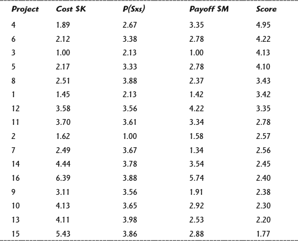
In most cases, the project data will be in units that vary in magnitude: probabilities to the right of the decimal, monetary costs to the left of the decimal, scale rankings in integers, and so forth. It is necessary to convert all the factors to a common range of values. Consider Table 2.6, with a portfolio of proposed projects. The magnitudes of the factors range from 3 digits to the left of the decimal to 2 digits to the right of the decimal. It is customary to standardize the project data by subtracting from each value the average of that value over all projects, and dividing that by the standard deviation of the value over each project. In terms of Table 2.6, this means subtracting from every value in a column the mean value of that column, then dividing the result by the standard deviation of the same column. Once the project-specific data have been loaded into a spreadsheet, this standardization process is trivial. It is as easy for a thousand projects as for a dozen.
Assuming the project-specific values are approximately normally distributed, the result should be standardized values ranging from about −3 to about +3. These must now be restored to positive values. If any of the original values in a column was zero, the standardized value for that factor should also be zero. Add to every value the absolute value of the most negative number in the column resulting from the subtraction and division process. This will result in standardized values ranging from zero to approximately 6. If none of the original values was zero, add to every number 1 plus the absolute value of the most negative number. This will give values ranging from 1 to approximately 7. These standardized values should then be substituted in the model. Each project then receives a score based on weights supplied by management, and project data supplied by the project originators (and possibly by other departments).
Table 2.3 shows the results of the model applied to standardized scores from Table 2.6. The rows have been re-ordered in decreasing magnitude of the score. If the standardized values are available in a spreadsheet, the process of computing project scores is trivial. Likewise, sorting the projects in order of scores is readily accomplished using a spreadsheet. In this example, Project 4 is the highest-ranked project. The other projects fall in order of their score. The next step would be to approve projects starting from the top of the list and working down, until the budget is exhausted. Note that the difference between projects 8 and 1 comes only in the third significant figure. Since most of the original data was good only to one or two significant figures, this difference should not be taken seriously.
Utilizing Scoring Models
When to Use. While these methods can be used for any type of project, they are especially useful in the earlier phases of a project life cycle when major project selection decisions are made. Take, for example, new product development projects. In the earlier project phases, market payoff is distant or even inappropriate as a measure of merit. In such projects, considerations such as technical merit—a frequent criterion in the Scoring Models—may be of greater significance than economic payoff. Selection of other types of projects, large and small, widely relies on Scoring Models as well. The final score is typically used for two purposes:
Table 2.3: Results of Applying Scoring Model to Example Data
Go/kill decisions. These are located at certain points within project management process, often at the ends of project phases. Their purpose is to decide which new projects to initiate and which of the existing ones to continue or terminate.
Project prioritization. This is where resources are allocated to the new projects with a “go” decision, and the total list of new and existing projects, which already have resources assigned, are prioritized.
For a comparison of Scoring Models and the Analytic Hierarchy Process (AHP), two project ranking tools that we cover, see the AHP section later in this chapter.
Time to Use. Although the principles behind the Scoring Models are relatively simple, developing an effective Scoring Model can be a very lengthy and time-consuming endeavor. In an example, it took a company several years to carefully select, word, operationally define, and test each criterion for validity and reliability. This detailed Scoring Model included 19 criteria and was designed to rate projects of strategic stature. Applying a model like this to sort through, rate, and rank a larger group of projects can easily take more than day or two of each decision maker's time. In contrast, some decision makers use off-the-shelf Scoring Models for the evaluation of their smaller, tactical projects, typically spending several hours on the scoring effort (see the “Tips for Scoring Models” box that follows).
Benefits. The value of the Scoring Model is that it can be tailored to fit the decision situation, taking into account multiple goals and criteria, both objective and judgmental, which are deemed important for the decision [2]. This prevents putting a heavy emphasis on financial criteria that tend not to be reliable early in the project life. With such an approach, decision makers are forced to scrutinize each project on a same set of criteria, focusing rigorously on critical issues but recognizing that some criteria are more important than others (by means of weights). Finally, the Scoring Model can be subjected to sensitivity analysis, by determining how much change in a weight would be required to change the priority order significantly.
Advantages and Disadvantages. Views about advantages and disadvantages of Scoring Models are not in short supply. Consider the following advantages:
- They are conceptually simple. They trim down the complex selection decision to a handy number of specific questions and yield a single score, a helpful input into a project selection effort. This is perhaps a major reason for models' wide popularity.
- They are completely transparent. This is in the sense that anyone can examine the model and see why the priority ranking came out as it did.
- They seem to work. Several studies showed that they yield good decisions. Procter & Gamble claims that their computer-based Scoring Model provides 85 percent predicative ability [1].
- They are easy to use. Managers involved in project selection rated scoring models best in terms of ease of use and deemed them highly suitable for project selection.
Tips for Scoring Models
Empirical evidence suggests that leading organizations favor approaches like this in using Scoring Models [1]:
- Have senior managers do scoring. There seems to be major bias in the selection process when project teams do the scoring, perhaps for favoring their projects.
- Make it discussion forum. The use of the model in a meeting format provides a benefit of executive buy-in, because senior managers examine each project together, discuss it on each criterion, rate it, and build a group consensus.
- Use a visible scorecard. When each decision maker has an electronic keypad, he or she can vote anonymously, have his or her votes instantly fed into a computer, and group results displayed on a large screen.
When it comes to disadvantages, there are beliefs that Scoring Models suffer from the following [1]:
- Imaginary precision. Using the models implies that the scores are highly precise, which simply is not the case—scoring is often arbitrary. This is why they should not be overused nor their results taken for granted.
- Potential lack of efficiency of allocation of scare resources. The issue here is that the models do not constraint the necessary resources when maximizing the total score for the project, as some Economic Methods do.
- Time-consuming. This disadvantage should be viewed in the light of the importance of the decisions. Were the decisions really crucial, extra time should be spent on them.
Variations. Major variations in using the models are closely linked to their time-consuming nature. In attempts to reduce the necessary time for project selection, companies took different paths. Unlike the approach of executive scoring of projects in the meeting, some companies first ask decision makers in the meeting to sort through projects and divide them into several groups of importance, then go to individual voting within the groups. Others rely on individual evaluators scoring before they come to the meeting. The purpose of the meeting is no more than seeing the results and discussing them. While this is a very time-efficient approach, it deprives the decision makers of the benefit of walking through each factor as a group, debating it, and building a consensus. Rarely, some organizations have project teams do prescoring of the project and present it to the decision makers, who accept or disprove the scores.
Customize Scoring Models. Although very beneficial tools, Scoring Models that we covered are of generic nature and, therefore, need to be adapted to account for a company's specifics and projects. Following we offer several ideas how to go about the adaptation.
| Customization Action | Examples of Customization Actions |
| Define limits of use. | Use Scoring Models for both large and small projects. |
| Use Scoring Models in new project selection and go/kill reviews of the existing projects. | |
| Adapt a feature. | Present briefly each project proposal to the decision makers before they engage in group discussion and rating of projects (helps busy decision makers). |
| Leave out a feature. | Do not use weights for criteria in very small projects in multiproject environment. |
- Check to make sure that a Scoring Model is appropriately structured and applied. It should:
- Be based on project proposals, strategic and tactical plans, and historical information.
- Include relevant criteria with weights and rating scale.
- Score each project on each criterion, multiply scores by weights and sum them across all criteria.
- Yield a single score for each project.
- Provide ranking of projects.
Summary
Presented in this section were Scoring Models, a project selection tool. These tools help assign scores to projects on a list of criteria. The score represents the merit of the project. Higher scores designate projects of higher merit. While these methods can be used for any type of project, they are especially useful in two situations: first, in the earlier phases of a project life cycle when major project selection decisions are made and projects prioritized, and second, in go/kill decisions. The key points in structuring and applying the Scoring Models are provided in the box that follows.
Analytical Hierarchy Process
What Is the Analytic Hierarchy Process (AHP)?
The Analytic Hierarchy Process (AHP), like the Scoring Model, provides a means for ranking projects. However, the Scoring Model is a “one-level” process. If one or more of the criteria are made up of subcriteria that are combined to get the value for that factor, this combining must be done outside the model. By contrast, the AHP specifically includes means for incorporating the combination of subcriteria. The procedure thus uses a “hierarchy” of criteria, with each criterion being disaggregated into sub-criteria corresponding to one's understanding of the project ranking situation (see Figure 2.3). Such breakdown offers an opportunity to seek cause-effect explanations between goal (e.g., select the best project), criteria (e.g., technical merit), subcriteria (e.g., probability of technical success), and candidate projects. Once this hierarchical structure is established, AHP continues with weighting of criteria and subcriteria and scoring that computes a composite score for each candidate project at each level as well as an overall score. The overall score signifies the merit of the project with higher scores representing projects of higher merit.
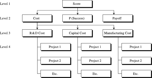
Figure 2.3. An example of the AHP decision hierarchy.
Applying AHP
The description of the AHP is, unfortunately, highly abstract. To make it more concrete, it will be illustrated using the same project menu and project selection criteria as were used for the scoring model.
Define the Problem and Goal. AHP's first step is to define the problem and determine the goal [3]. In our case the goal is known—we want to rank the new and existing projects so that we can select the best new ones to initiate or continue/terminate them if they are already in existence.
Collect Information Inputs. Like Scoring Models, AHP starts with the need to have a list of candidate projects to select from and quality information inputs to perform ranking. The inputs are as follows:
- Project proposal
- Strategic and tactical plans
- Historical information.
As explained in the “Scoring Models” section, these inputs ensure understanding of the company's strategy and goals, project goals and scope, and the results of past project selection decisions and past project performance.
Construct the Hierarchy. As with any other project selection method, it is necessary to decide on the criteria that will be used to rate projects. The unique feature of AHP is that the criteria are disaggregated into as many sublevels as needed for each criterion. To illustrate this, we will use the same criteria as we did for the Scoring Model. We wish to rank projects according to their merit, taking into account Cost, Probability of Success, and Payoff, with Payoff having twice the weight of Probability of Success and Cost. The hierarchical model is given in Figure 2.3. To illustrate that subcriteria can be included, the Cost criterion has been subdivided. However, since that data is not available in Table 2.3, the actual computation will not involve the subcriteria. Instead, the projects will be evaluated against the each of the lowest-level criteria, in our case Cost, Probability of Success, and Payoff. That is, projects would be evaluated against all three elements of cost (if these were available), as well as against Probability of Success and Payoff.
Construct Comparison Matrices. At each level of the hierarchy, a matrix must be developed whose elements are the relative preference (weight, significance, value, etc.) for each criterion at that level as compared with all the other criteria at that same level. The entries in the matrix show the degree to which the Row factor is preferred to the Column criterion.
To continue the example using data from Table 2.3, we develop the first-level comparison matrix. At the first level of the matrix below the total score, the three factors are Cost, Probability of Success, and Payoff. The matrix is as follows:
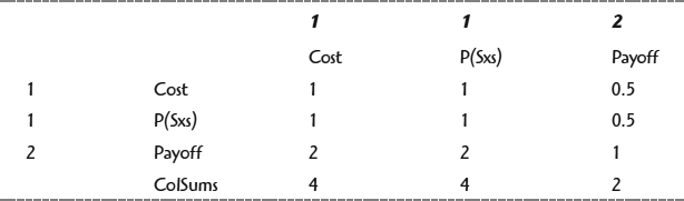
The relative weights of the three factors are shown in the top row and the extreme left column. The degree of preference is shown in the cells inside the double line. In the row for Cost, it is shown as having half the preference as Payoff, in the Payoff column. The diagonal elements, of course, are all 1, and the elements below the diagonal are the reciprocals of their corresponding elements above the diagonal. Thus, in the row for Payoff, the cell entry in the column for Cost is 2, showing that the preference for Payoff is twice that for Cost.
In this example we had definite numbers for the relative preferences. However, in many cases, the elements of the matrix must be developed judgmentally. The process of developing each matrix can be very time-consuming. It is important to note, however, that not all the matrices in the hierarchy need to be developed by the same people. For instance, in this model, the relative likelihood of project success matrix might be filled out by technical management, the payoff matrix by marketing, and the cost matrix by executives from personnel, purchasing, and other relevant departments.
Next, a new matrix is formed in which the elements are the elements of the above matrix, all divided by their column sums:
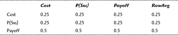
The row averages are the weights that will be used to multiply the respective results of a similar operation on the values of Cost, Probability of Success, and Payoff for each of the projects.
A similar matrix of preferences is developed for each factor, over all projects. A portion of the Cost matrix follows. Note that since a higher cost is less preferred than a lower cost, the column cost is divided by the row cost to obtain the cell entry of preference of row for column for each project. To save space, only the upper left corner of the entire array is shown. Similar arrays for Probability of Success and Cost follow. Since for these factors a larger value is preferred to a smaller value, row weight is divided by column weight to obtain preference of row factor for column factor.
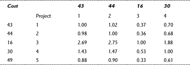
Here again we have definite numbers to start with, and the computation of the matrix is trivial if a spreadsheet is used. In many cases, however, the matrix must be filled in judgmentally. Since this is a 16×16 matrix, n(n−1)/2 or (16×15)/2 = 120 judgments would be required. (The entries below the diagonal should be the reciprocals of their mirror-image elements above the diagonal, and diagonal elements are always 1.) This can be a major effort on the part of the people responsible for rating the projects on this particular criterion
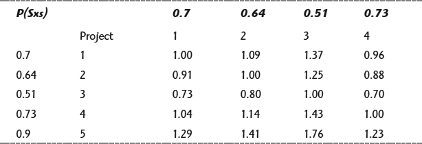
A portion of the matrix for relative preferences of Probability of Success is shown in the following. Note that since a higher probability is preferred to a lower probability, row probability is divided by column probability to obtain relative preference for a row.
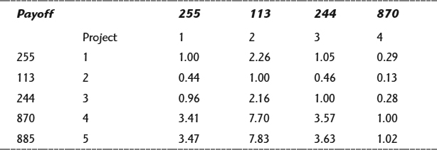
The Payoff matrix, which follows, is developed in the same manner. Like the Probability of Success matrix, higher payoff is preferred to lower, so row payoff is divided by column payoff to compute a cell entry.
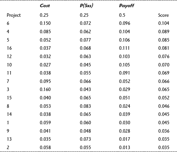
Compute the Rating. As was the case with the array of preferences for the three criteria, now each column of the three project preference arrays is divided by its column sum, and the row averages are computed. Table 2.4 shows the row averages for each factor (inside the double lines), the weights for each factor computed at the first step (across the top), and the final scores for each project in the rightmost column. The scores are computed by multiplying the top row by the row for the project and summing. The projects have been sorted in decreasing order of score. As with the Scoring Model, once the criteria matrices have been generated by management and the project-specific data generated by the project teams or other appropriate groups, the final computation of the scores is trivial if a spreadsheet is used.
Utilizing AHP
When to Use. AHP was not designed specifically to assist in project ranking. Rather, it was developed to facilitate sound decision making, whatever the decision problem is. Consequently, its realm in projects goes far beyond project ranking to include ranking alternatives and making decisions in all knowledge areas of project management. Consider, for example, selecting the best among several candidates for the project manager position. Choosing the best among multiple vendor bids is another example. Still another would be selecting the best among four possible ways to accelerate the project that is significantly late. Apparently, the opportunities to apply AHP in project management are numerous. In all of them multiple alternatives are available and AHP's job is to help rank them and choose the best. In this sense, AHP's purpose is to reduce the risk by selecting the best alternatives. This is why AHP is considered a decision and risk analysis tool, included here because its major current application is in project selection.
Aside from this, AHP is generally used in larger, more important projects for new project selection and go/kill reviews of the existing projects [4]. Helpful in this are specialized software tools such as Expert Choice or Automan, or Excel. While in smaller decision problems using AHP may be an individual exercise, the real value of AHP lies in a group decision-making environment (see the box titled “Tips for AHP” coming up in the chapter). This is particularly important when the data for different subcriteria will be generated by different groups. Instead of a group of experts in disparate disciplines trying to come to a consensus, AHP allows experts in each discipline to fill out the relevant matrices, using their disciplinary expertise. The results can then be combined with the results from other groups, using the AHP.
Table 2.4: Final Project Rankings Obtained with the Analytic Hierarchy Process
Comparison of the Scoring Models and AHP
How do the results of Scoring Models and AHP compare? The following table gives the rank order of each project in the example, as determined by the two methods (repeating the scores shown previously):
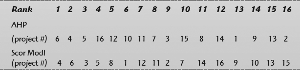
Although in many cases the two methods are in good agreement, that is not the case in this example. The methods are in close agreement on the first and second rank projects. From then on, however, the two methods disagree significantly. The correlation coefficient for the two sets of ranks is only 0.14. Which method is right? There is no way to tell. If we had some objective measure of merit for projects, we wouldn't be using these methods. The important consideration is that each of these methods has strengths and weaknesses. The Scoring Model is easier to use. However, it is a one-level process that ignores finer divisions of factors. The AHP is more complex to use (although with a spreadsheet the calculations are quite simple), but it does take into account the hierarchy of factors. If ease of use is important, the Scoring Model is the better choice. If the decision involves factors that can be disaggregated into lower-level factors, and this desegregation is important, the AHP is the better choice. Recognize, however, that there is no way of knowing which is “right.”
Time to Use. The time required depends on whether objective data (monetary costs, staff hours, machine time, etc). can be available, or whether the various matrices must be filled out judgmentally. Where objective data can be made available, the time required is only that for gathering the data. Computing the matrices using a spreadsheet is trivial. If the matrices must be filled out judgmentally, however, the effort can be very time-consuming on the part of management, who are responsible for deciding on the criteria and the relative importance of these criteria. For example, developing and applying a simple hierarchy with three levels and several factors per level may take a group of a few decision makers several hours. Situation changes radically when hierarchy has five levels with tens of criteria involved, driving the necessary time to tens of hours for each involved decision maker. Note, however, that in either case once the matrices are available, the only new information required every time the method is used is project-specific data. Management effort is thus a one-time activity and need be repeated only when external conditions demand a change in the matrices. Making use of a well-trained facilitator significantly improves time performance.
Benefits. AHP provides value on multiple levels beginning with the ability to marry simplicity with complexity. By breaking complex problems such as the project ranking into levels, AHP helps focus on smaller parts of the problem, thinking about one or two criteria at a time. As evidence from the proverbial Miller's Law suggests, humans can compare only 7+-2 items at a time. AHP's focus on a series of one-on-one comparisons of criteria, for example, then synthesizing them further improves the quality of decision. Such an approach enables the decision maker not only to arrive at best decision but also provides the rationale that it is the best. AHP's ability to handle complex situations in an easy way is based on the use of multiple criteria, some of which are subjective, while others are objective aspects of a decision. The subjective aspects may include qualitative judgments based on decision makers' feelings and emotions as well as their thoughts. On the other hand, the objective aspects may address quantitative criteria such as profitability numbers. AHP's flexibility of juggling simultaneously both objective and subjective, quantitative and qualitative aspects is unmatched. It truly ensures a systematic, all-angle project ranking, or more generally, risk reduction in decision making.
Advantages and Disadvantages. AHP offers powerful advantages captured in:
- Simple procedure. The procedure lays out a simple and effective sequence of steps to arrive at project ranking, even in group decision making when diverse expertise and preferences are involved.
- Visual hierarchies. Complex decision problem of project ranking is represented with graphical hierarchical structures. Even when the structures are elaborate, they make the problem visual, simplifying potential risk and conflict [5].
- User friendliness. The availability of computerized tools has simplified the mathematical procedure, eliminating the once insurmountable process of computations.
Disadvantages are related to AHP's:
- Subjective nature. This is because different decision makers can assign different levels of importance to a particular criterion.
- Complexity. As the number of criteria increases, the tabulation and calculations become complex and also tedious.
- Difficulty. Some users feel that quantifying the importance of some criteria may turn out difficult at times.
Variations. The approach used in AHP is very similar to another tool called MOGSA (Mission, Objectives, Goals, Strategies, Actions), an example of which is shown in Figure 2.4 [6]. MOGSA also uses the hierarchical breakdown of the decision problem to build a network of relationships among three major levels of the hierarchy: impact level (M, O), target level (G), and operational level (S, A). Where MOGSA differs from AHP is in some computational aspects.
The following approaches can help in using AHP:
- Have senior managers select the criteria. The criteria reflect the firm's strategy and goals.
- Make it a discussion forum. If the relative preferences in the upper-level matrices must be obtained judgmentally, using a meeting to generate them helps obtain executive buy-in, because senior managers examine each criterion and judge relative importance.
- Use disciplinary teams for judging specific matrices. Since the AHP allows disaggregation of criteria, using experts on each criterion improves the results of judgmental comparisons.
- Use a visible display. When all participants have electronic keypads, they can vote anonymously, have their votes instantly tallied by a computer, and group results displayed on a large screen. Reasons for altering the relative preference can then be discussed.
Customize AHP. Think of AHP described here as a generic one. You can significantly enhance its value by adapting its use to the specifics of your project situation. A few simple ideas given in the following are no more than clues in that direction.
Summary
AHP was the topic of this section. Although most widely used in larger, more important projects for new project selection and go/kill reviews of the existing projects, AHP is used for ranking alternatives and making decisions in all knowledge areas of project management. In all of them multiple alternatives are available, and AHP's job is to help rank them and choose the best. The value of AHP lies in its ability to deal with complex situations in an easy way. In doing so, AHP handles both objective and subjective, quantitative and qualitative aspects. The following box highlights key points in structuring and applying AHP.
| Customization Action | Examples of Customization Actions |
| Define limits of use. | Use AHP in larger, strategic projects for new project selection, and go/kill reviews of the existing projects (use professional software and facilitator). |
| Use AHP as a risk-planning tool in evaluating several alternative approaches within the project (schedule, cost, hiring alternatives). | |
| Adapt a feature. | Stick with simple hierarchies (levels 1, 2, and 3) when using AHP as a risk planning tool within the project (rely on Microsoft Excel for this). |
| Use anchored scales for making judgmental preferences because it aids participants in making consistent judgments. |
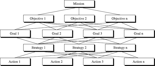
Figure 2.4 An example of the MOGSA (Mission, Objectives, Goals, Strategies, Actions) decision model.
Economic Methods
What Are Economic Methods?
Economic Methods are designed to take into account monetary cost and return from projects. They thus tend to ignore technical merit and similar considerations. Rather, they are intended for use when economic considerations are paramount. However, only financial data are required, which simplifies their use.
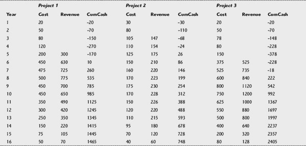
Three different economic models will be presented: Payback Time, Net Present Value (NPV), and Internal Rate of Return (IRR). Table 2.5 presents three hypothetical candidate projects, with their associated cost and revenue streams. These projects will be evaluated using each of the three Economic Methods.
AHP Check
Check to make sure that AHP is appropriately structured and applied. It should:
- Be based on project proposals, strategic and tactical plans, and historical information.
- Structure the hierarchy: the top (goal: select best projects)—intermediate levels (selection criteria, subcriteria)—lowest level (candidate projects).
- Construct a set of pairwise comparison matrices for each of the lower levels.
- Do relative scores within each level of the hierarchy.
- Yield a single score for each project on each level and an overall score.
- Rank projects according to final rating.
Payback Time
Payback Time is simply the length of time from when the project is initiated until the cumulative cash flow (revenue minus costs) becomes positive. At that point all the funds invested in the project have been recovered. As can be seen from Table 2.5, the cash flow for Project 1 turns positive in 6 years, for Project 2 in 5 years, and for Project 3 in 8 years. By this criterion, Project 2 is the best choice.
Payback Time is a very conservative criterion and provides more protection against future uncertainties than do either of the other Economic Methods. However, it is insensitive to project size, since a project with massive investment requirements may still have short Payback Time. Moreover, it takes no account of future potential once payback is reached. Both Projects 1 and 3 have greater future income than Project 2, but the initial investment before payback is greater and the time for cash flow to turn positive is greater.
Net Present Value
Net Present Value (NPV) takes into account the time value of money, in that a dollar a year from now is worth less than a dollar today. NPV discounts both future costs and revenues by the interest rate, according to the formula:
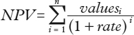
In this formula, values represent the sum of costs and revenues in year i, and rate is the discount rate or the rate the company pays for borrowed money, expressed as a decimal fraction.
Excel and other spreadsheets compute NPV directly. You only need to enter the discount rate and the values (or a vector of cells) into the NPV function. The result is computed and displayed in the cell holding the function. Using the NPV function, the NPV for each of the three projects, at discount rates of 5 percent, 10 percent and 15 percent, are as shown in the following table:
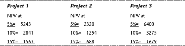
Table 2.5: Candidate projects for Payback Time Evaluation
The more the future is discounted (i.e., higher discount rate), the less the NPV of the project. At all discount rates, Project 3 is superior to the other two projects. That is, the higher the NPV, the higher the ranking of the project.
NPV takes into account the magnitude of the project and the discount rate. It is not a particularly conservative measure, however, since it incorporates estimated future revenues that may not actually materialize.
Internal Rate of Return
Internal Rate of Return (IRR) is simply the discount rate at which NPV for the cash flow is zero. There is no closed-form formula for it. IRR must be computed iteratively, “homing in” on the exact discount rate that produces an NPV of zero. Most spreadsheets, however, have an IRR function that allows the user to obtain IRR. You need enter only the list of values (or a vector of cells) and a guess value of IRR. The function then carries out the iterative calculation.
For the set of candidate projects, the IRR values are as follows:
| Project | IRR |
| 1 | 42% |
| 2 | 40% |
| 3 | 36% |
By the IRR criterion, Project 1 is superior to the other two projects. While IRR discounts future values, it takes no account of the size of a project. Project 3 promises a significantly greater total return than Project 1, but those returns are farther in the future and follow a longer course of investment before cash flow turns positive. Hence, the IRR for Project 3 is lower than that for Project 1.
Choice of Economic Method
As this example shows, the three methods can give differing results on the same set of projects. Which method should be chosen depends on the considerations important to the decision maker. NPV favors projects with large payoffs but gives little protection against future uncertainties. IRR likewise gives little protection against future uncertainties and may tend to give preference to a project with modest total payoff but high return on a modest investment. Payback time is a very conservative method, giving more protection than the other two methods against future uncertainty, but it takes no account of size of project payoff, nor of the discounted value of future costs and revenues. Whichever consideration is most important will govern the choice of methods. Moreover, since these methods treat projects as capital investments, it would be appropriate to use whichever method the company uses for evaluating its other capital investments, thus allowing a direct comparison between projects and other investments.
Tips for Using Economic Methods
| This provides a direct comparison between the project and alternative investments. | |
| This neither favors nor works against the proposed project, by comparison with alternatives. | |
| Check what happens with different discount rates or different scenarios of costs and revenues. |
Utilizing Economic Methods
When to Use. Economic Methods require data about revenues and costs expected to result from the project. They are thus appropriate primarily for capital projects and projects intended to improve existing products or develop new products. In such cases they allow a direct comparison of such projects with alternative capital investments. For a comparison of the three methods, see the box on page 44, “Choice of Economic Method.”
Time to Use. The time required to use any of these Economic Methods is primarily that required to gather the future cost and revenue data. That can take hours for smaller projects or tens of hours in larger projects. Once the data have been obtained, any of the methods can be calculated readily using a spreadsheet.
Benefits. Economic Methods are readily understandable. They enable the decision maker and project managers to communicate more readily about financial considerations of projects. They also make it easier to compare projects with other opportunities for capital investment. Once the necessary data are obtained, they are easy to compute. They also make sensitivity testing easy. Alternative scenarios about future costs and revenues can be compared to see how robust a selection of projects is against future uncertainty. See the “Tips for Using Economic Methods” box above.
Advantages and Disadvantages. The primary advantage of Economic Methods is that they are their relatively straightforward. Like in all capital investments, their disadvantage is that they require data about future costs and revenues. Not only may these be difficult to obtain, but also they may be subject to considerable uncertainty.
Summary
Presented in this section were three Economic Methods for project selection: Payback Time, Net Present Value, and Internal Rate of Return. They are appropriate primarily for capital projects and projects intended to improve existing products or develop new products. In such cases they allow a direct comparison of such projects with alternative capital investments. They are readily understandable and once the necessary data are obtained, they are easy to compute. We recapture the key points for applying the Economic Methods in the box that follows.
Check to make sure that Economic Methods are appropriately applied. You should:
| These estimates should be made as far into the future as the project is likely to be generating either costs or revenues. | |
| Use the method that is used by the firm for other capital investments. | |
| For a single project, a spreadsheet is adequate for computing any of the three Economic Methods. | |
| Test the results against more optimistic and more pessimistic streams of costs and revenues, and against higher or lower interest rates on borrowed funds. |
Portfolio Selection Methods
What Are Portfolio Selection Methods?
The methods presented in the previous sections treat each project in isolation, without regard to interactions with other projects. In fact, there may be constraints that limit choice of projects. The most obvious constraint is the budget. However, there may be other constraints operating besides the financial budget. Staff limitations, limitations on supporting activities such as model shop time or computer time, and other considerations such as company policy may constrain the choice of projects. To deal with these issues, Portfolio Selection methods must be used [7]. These take into account all the constraints that may be operating to limit the choice of projects.
Applying Portfolio Selection Methods
Collect Inputs. The major inputs include the following:
- Data about candidate projects
- Company policies
The first step in applying Portfolio Selection methods is to identify the set of projects that are candidates for inclusion in the portfolio. It is then necessary to collect data about each of the candidate projects. The data must include those items that represent potential conflicts or interactions among projects. Overlapping resource requirements, company policies about types of projects to be included in the portfolio, and other items that might limit the possible combinations of projects must be collected.
Construct the Portfolio Model. Consider the project menu in Table 2.6. In addition to the selection criteria used in the Scoring Model and AHP examples, we will take interactions among the projects into account to obtain a portfolio with no conflicts. Assume there is a budget limitation of $600 K, there are only 4500 Model Shop hours available, and only 700 hours of computer time available. Within these constraints, you wish to select projects that will maximize Payoff.
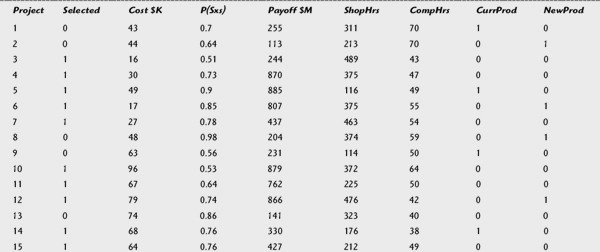
Spreadsheets such as Excel can perform this “optimization” for small-sized problems. Table 2.7 shows an Excel spreadsheet set up to carry out the Portfolio Selection that maximizes payoff while not violating any of the constraints. An entry of 1 in the “Selected” column indicates which projects have been selected as part of the portfolio. Cell entries of 0 mean the project has not been selected. The Total Cost cell entry is simply the Excel SUMPRODUCT function of the Selected column and the Cost column. Similarly for the Model Shop Hours and the Computer Hours.
Once the problem is set up using Excel SOLVER (or the equivalent in other spreadsheets), the optimum portfolio can be calculated directly. As can be seen in the table, the Total Cost, Model Shop Hours, and Computer Hours satisfy the constraints imposed. The remaining constraints need some explanation. We do not want the spreadsheet to try to “buy” resources by selecting a “negative project.” Hence, we must constrain the entries in the Selected column to be equal to or greater than zero. We also do not want the “optimum” solution to contain multiple copies of the most profitable project. Hence, we must constrain the values in the Selected column not to exceed 1. Finally, we can't buy half a project; hence, the values in the Selected column must be constrained to be integers. The three constraints acting together ensure that the values in the Selected column will be either 1 or 0, or in other words, that whole projects will be selected a maximum of one time each.
It is possible that there might be two versions of the same project in the candidate list, a “crash” version and a “normal” version. We would want to select only one of these; hence, another constraint would have to be added:
![]()
where X and Y are the cells in the Selected column corresponding to the two versions of the same project.
Table 2.6: Candidate Projects for Scoring Models and Portfolio Optimization Methods
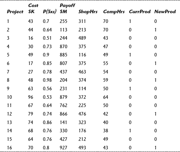
Suppose further that there is a company policy that at least one project must support an existing product and at least one project must support a new product. The two rightmost columns in the table have entries of 1 to indicate whether a project supports a new or existing product or whether it is not product-related (it might be a manufacturing improvement project). We could add constraints that the SUMPRODUCT of the Current Product and the SUMPRODUCT of the New Product columns with the Selected column must equal or exceed 1. In the preceding example, this would not alter the outcome, since projects that support current and new products are already in the solution set. However, had that not been the case, and we added those two constraints, some other projects would be forced into the solution set. The result would most likely have been to reduce the total payoff, but to satisfy company policy.
In this example, the budget turns out to be the binding constraint. The projects in the solution set consume almost the entire budget. By contrast, there is a considerable margin left in both Model Shop hours and Computer hours. This opens the possibility of some sensitivity testing. How much more would the total return increase if the projects budget were increased? No matter which is the binding constraint, use of the optimization capability of a spreadsheet will allow the decision maker to determine how much additional return can be obtained from relaxing the binding constraint, or conversely, how much return will be lost if a constraint is made more binding.
Table 2.7: Portfolio Selection that Maximizes Payoff While Not violating Any of the Constraints

Utilizing Portfolio Selection
When to Use. Portfolio Selection should be used when there are multiple constraints on the selection of projects (see the “Tips on Portfolio Selection” box that follows). Since some measure of payoff is required for the optimization, it is most easily used when the objective is to maximize revenue. However, it can also be used for types of projects that do not involve direct revenue generation. For instance, a list of candidate projects could have figures of merit developed through either a Scoring Model or the AHP method. The Portfolio Selection could then maximize the sum of the figures of merit subject to constraints on financial budget, staffing, support activities, and other resources. That is, the figure to be maximized need not be financial revenue. It can be any measure of goodness of the candidate projects, whether they are larger or smaller projects.
Time to Use. The time required for use of Portfolio Selection is primarily that of collecting the data for the candidate projects. Setting up the problem on a spreadsheet is fairly simple, and the time required for carrying out the optimization is negligible. However, spreadsheets are suitable only for small optimization problems. If the candidate list is large or there are many constraints, a spreadsheet may be inadequate. In this case some more powerful optimization procedure may be needed. If the task is large enough or complex enough, there may be no alternative but to use a specialized optimization program on a mainframe computer. In such cases, the time to set up the problem, run the program, and check validity can become significant.
Benefits. As compared with other project selection methods, Portfolio Selection takes into account the interactions among projects and allows the decision maker to specify the constraints the portfolio must satisfy [8]. These may include limits on the utilization of particular resources or conformance to company policy about the types of projects that must be included in the portfolio. As a result, a portfolio of projects does not have any built-in conflicts over resource use or conformance to policy.
Tips on Portfolio Selection
- Higher management should set the optimization criteria. Only higher management is in a position to know what should be optimized (financial return, technical merit, or other).
- The responsible departments should establish the constraints. Since the constraints may be other than financial, the departments responsible for the limiting resources should determine the constraints.
- Higher management should establish any policies that must be satisfied. If there are policy considerations to be taken into account by the portfolio optimization, these must be established by higher management, which is the only authority capable of establishing them.
Advantages and Disadvantages. For small optimization problems, Portfolio Selection is a relatively easy application. By contrast, optimization problems with a large list of projects and many constraints have the disadvantage that more data may be required for them than for other project selection methods. This makes the data collection process more time-consuming and costly.
Customize Portfolio Selection. Like with our tools, Portfolio Selection will provide more value if the generic version we have covered is customized to your specific project situation. A few simple ideas given in the following may help provide direction for such an effort.
| Customization Action | Examples of Customization Actions |
| Define limits of use. | Use Portfolio Selection when there are multiple constraints on the selection of projects (e.g., budget and resource conflicts). |
| Include both revenue-generating and non-revenue-generating projects (convenient for both small and large companies). | |
| Adapt a feature. | Keep the optimization problem small (rely on Excel spreadsheet for this). |
| Keep the number of constraints to a minimum (this is convenient for small companies with limited resources). |
Portfolio Selection Check
Check to make sure that Portfolio selection is appropriately applied. You should:
- Collect cost and other relevant data on each project. For each candidate project, collect data on each of the criteria by which the projects might be evaluated.
- Identify potential conflicts among projects. Identify uses of limited resources over and above the financial budget that might constrain the possible combinations of projects.
- Identify company policies that might constrain combinations of projects. Determine whether company policies require certain types of projects to be included in the portfolio, or forbid certain combinations of projects.
- Set up the optimization problem. If the problem is sufficiently small, use a spreadsheet. Otherwise, use a more powerful program on a mainframe.
- Identify the optimum portfolio. Run the optimization, and determine which combination of projects satisfies all the constraints.
- Test sensitivity. Determine how much change in any constraint is required to alter the project portfolio.
Summary
This section reviewed Portfolio Selection, a project selection tool used when there are multiple constraints on the selection of projects. It is most easily used when the objective is to maximize revenue. However, it can also be used for types of projects that do not involve direct revenue generation. Thus, it can be any measure of goodness of the candidate projects, whether they are large or small. Compared with other project selection methods, Portfolio Selection has an advantage of taking into account the interactions among projects and allowing the decision maker to specify the constraints the portfolio must satisfy. Recapturing the core of the application are checkpoints in the box that precedes.
Real Options Approach
What Is the Real Options Approach?
Basic research projects are inexpensive enough that they can be carried as overhead. Product development projects are expensive enough that they must be treated as a capital investment and looked at as being in competition with other capital investments projects the company can make. There is, however, an intermediate type of project that is too large to be treated as overhead but not yet ready to be treated as a capital investment. The appropriate approach to projects of this type is to treat them as options.
Analogy with Financial Options. The Real Options Approach is a relatively new method of project selection that uses analogy with financial options. To make it clear, we will first explain the analogy, before moving to lay out its use. An option is a financial instrument used to “lay off” risk to some other party willing to bear that risk for a price. The two option types are the put and the call.
Suppose you hold some shares of a specific stock. You want to continue holding them for the long term, but if the investment turns sour, you would like to limit your loss. One way to do this is buy a put option. This allows you to sell the stock at a specified price during a specified period of time. If the stock drops below the “strike price” before the option expires, you can sell it at the specified price, regardless of how much lower the market price has fallen. Clearly, the person selling you the put is betting that the price of the stock will not drop below the price specified in the put. For assuming the risk that the price will drop below that value, he or she is charging for the put. The price for a put depends on both the buyer's and seller's estimates of the risk that the option will be exercised. From the buyer's standpoint, the put is a way of reducing downside risk.
Suppose conversely that you believe there is some probability, but not certainty, that the price of a specific stock will increase. Or alternatively, you already own some of that stock on the basis of your belief that its price will increase, but you are hesitant to buy more. Still, in either case you would like to benefit from a price increase if it does occur. You can buy a call option. This gives you the right to purchase a specified number of shares of that stock at a specified price, during a specified period. If the price of the stock rises above the strike price during the option period, you can buy the stock at the specified price and resell it at a profit, or you can hold it for further profits. Clearly, the person selling you the call is betting that the price of the stock will not rise above the price specified in the call. For assuming the risk that the price will rise above that value, he or she is charging for the call. The price for the call depends on both the buyer's and the seller's estimates of the risk that the option will be exercised. From the buyer's standpoint, investing in the call buys an opportunity to make a further investment if the investment turns out to be profitable.
In the case of financial options, the key to how much a call or a put is worth is the volatility of the stock or other financial instrument in question. The more volatile the price of the instrument, the greater the chance that it will rise above, or fall below, the strike price, in which case the holder will exercise the option. An instrument with a low volatility—that is, one that is not likely to rise or fall very much in price—would involve only a low price for either a put or a call. In the case of financial instruments, the measure of volatility is the standard deviation of the price over some suitable period of time.
Applying the Real Options Approach
An intermediate project of the type described in the preceding text, too big to be carried as overhead but not ready to be treated as a capital investment, is analogous to a call in a financial market. Investing in the project amounts to buying an opportunity to make a further investment if that further investment turns out to be profitable. As with a financial investment, there are both upside and downside risks with such a project. The downside risk is that the project will not pan out. Everything spent on it will be lost. The upside risk is that it will turn out to be even more favorable than you anticipated, and you will miss out on some payoff that you could have obtained had you invested more.
Identify the Risks Associated with the Project. There are three kinds of risk the company may face in treating a project as an option. Each of these types of risk must be offset to the extent possible by one or another of the options described previously.
- Firm-specific risk. The risk that the firm will not have the funding, the technical skills, or other resources needed to carry out the project.
- Competition risk. The risk arising from actions under the control of competitors, such as preempting with a similar project.
- Market risk. The risk due to uncertain factors such as customer demand, regulatory changes, or emergence of a cheaper or substitute technology.
Offset Risks: Analogies to Puts and Calls. The put is a way of limiting losses from downside risk. The call is a way of gaining benefit from upside risk. If we are to treat a project as a call, we need to look for analogies to the financial put and call for reducing downside and upside risks.
Some measures that are analogous to puts are as follows:
- Defer. Postpone the project while gathering additional information about risks and payoffs.
- Multistage. A project that can be done in stages can be stopped if things look bad, and resumed if new information justifies resumption.
- Outsource. A contract with a third party to carry out the project. The contract can be terminated early (perhaps with a penalty fee) if the project begins to look bad. (Note that this creates the risk that you will be creating a competitor.)
- Explore. Start with a pilot or prototype project and expand it if it looks favorable.
- Lease. lease facilities from a third party, terminating the lease early (possibly with penalty fee) if the project begins to look bad.
- Abandon. Choose facilities or other equipment that have a high salvage value, so that something can be recouped if the project must be terminated.
- Flexible scale: design the project so that it can be contracted if conditions turn out to be less favorable than anticipated, but not so bad the project should be terminated.
Each of these measures serves to limit the downside risk of the project. Each costs something, but each either reduces risk or transfers that risk to someone else.
While the project itself is analogous to a call, there are other measures, also analogous to calls, that can enhance payoff if the project turns out to be more favorable than anticipated.
- Hedging. Make low-cost investments in additional facilities so they will be available if things turn out even better than expected.
- Flexible scale. Design the project so that it can be expanded if conditions turn out to be more favorable than anticipated.
There is yet another kind of option that the decision maker should consider:
- Strategic growth. This is a project that is a link in a chain of projects or is a prerequisite to other projects. Such a project can be considered a call, since it makes possible greater payoffs from favorable developments. However, it does not in itself produce a payoff.
Structure the Project to Manage Risk. The steps the decision maker should take in managing the risk are as follows:
- Define the project and identify the risks to which it is exposed. These must be specific risks, not generic ones (e.g., a specific competitor may come out with a comparable product).
- Recognize shadow options (i.e., options that the company might take) to reduce each of the specific risks identified in the previous step.
- Devise alternative ways to structure the project, each way involving different combinations of the shadow options identified in the previous step.
- Identify the combination of options that results in the most valuable project structure.
- Convert one specific set of shadow options into real options.
Defining the project means determining its goals and objectives, and identifying the specific risks that these goals and objectives will either not be met or that they will turn out to be inadequate if results are even more favorable than expected. Each specific risk must be controlled by choosing an appropriate option—a project put or call.
For each risk, the decision maker must identify at least one shadow option that the company might take in order to minimize or control that risk. The potential cost and benefit (degree of risk reduction) from each shadow option must be determined.
Once the shadow options have been determined, the decision maker must devise various project structures, each with a different combination of shadow options. The extent to which this development of alternative structures goes will depend on project size. The bigger the project and the greater the risks, the more effort is justified in defining alternative structures.
Once the alternatives have been devised, the decision maker must examine all the possible project structures and determine which is most favorable. That is, the decision maker chooses the project structure that provides the greatest opportunity to make a profitable investment at a later time.
The final step involves converting the shadow options of the chosen combination into real options. For instance, the shadow option to lease facilities becomes real when the company draws up bidding specifications and submits them to potential bidders. Each of the shadow options in the chosen project structure must be converted into real options. This may be costly, but the set of options, and the project structure, have been chosen to provide maximum protection against risk, as well as maximum benefit from the project itself. Failure to convert one or more shadow options to real options means exposing the project to the risks identified at the outset.
How much is it worth to the company to offset the risks accompanying the “call” of starting a project? In the case of financial instruments, the volatility of the price affects the price of the call. In the case of a project, the equivalent of volatility is the maximum potential for the project. The higher that maximum potential, the more the project is worth as a “call.” As the project progresses, the company must continually update its estimates of maximum potential. As the estimate increases or decreases on the basis of new information (e.g., a new government regulation decreases the size of the potential market and thus reduces the estimated potential, or a partnership with a foreign firm opens an additional market and increases the estimate), the project may require a new decision to terminate or continue.
This concept can be illustrated in Figure 2.5 [9]. Corresponding to the volatility of a financial instrument, the volatility of a project is the range of possible outcome values, that is, the maximum possible value minus the minimum possible value (which may, of course, be zero). The greater this range of possible outcomes, the greater the uncertainty associated with the project, but likewise the greater the possible payoff. A project with a large range of possible payoffs is thus a candidate with attractive possibilities for future further investments.
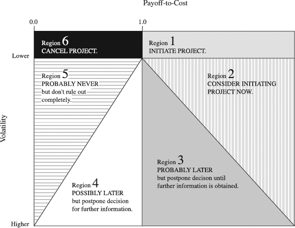
Figure 2.5 Dividing option space into regions.
From Timothy A. Luehrman, “Strategy As A Portfolio of Options,” Harvard Business Review, September–October 1998. Copyright © Harvard Business School Publishing. Reprinted with permission of Harvard Business School Publishing.
Another measure of the value of a project is the ratio of NPV of returns from the project if it achieves maximum payoff divided by the NPV of the costs to pursue the project. Call this ratio Payoff-to-Cost. The greater this ratio, the more attractive the project is.
Figure 2.5 illustrates the various combinations of Volatility and Payoff-to-Cost, and the decisions to be made in each case. Volatility increases from top to bottom; Payoff-to-Cost increases from left to right. The figure is divided into six regions, based on the combination of Volatility and Payoff-to-Cost. Each region calls for a different decision.
Regions 1 and 6 are the “easy” regions. In these regions, volatility is nearly zero (minimum payoff is close to or equal to maximum payoff), which implies that the payoff value is known with good precision. In Region 1, NPV of payoff is greater than NPV of cost, hence the project is a clear winner. In Region 6, NPV of payoff is less than NPV of cost; hence, the project is a clear loser.
In Region 2, Payoff-to-Cost ratio exceeds 1, and the volatility is low compared to Payoff-to-Cost. However, there is still some uncertainty. The project can be postponed, to await further information (perhaps a reduction in volatility); but if there is some benefit to starting it now as compared to waiting, then consider starting it now.
In Region 3, Payoff-to-Cost ratio exceeds 1, but the volatility is very high by comparison to Payoff-to-Cost. The project should be postponed to see if further information reduces volatility.
In Region 4, Payoff-to-Cost ratio is less than l. This weighs against the project. However, volatility is high, and if maximum payoff turns out to be high enough, the project might be moved into Region 3 or Region 2.
In Region 5, Payoff-to-Cost ratio is less than 1. This weighs against the project. Moreover, volatility is low, implying that there is little chance the project will ever become attractive. It should be kept as a potential project until further information resolves the issue of volatility.
Having viewed the implications of considering projects as options, we now look at an illustrative example of how to apply the concept of options to a project.
An Illustrative Example
Steps that we have described in applying the Real Options Approach will now be demonstrated in a real-world example. The Research Laboratory of Company X has shown the technical feasibility of a new consumer product. It is within the state of the art. However, considerable engineering work will be required before the idea is ready for product development. The decision has been made to investigate the possibility of treating the engineering development project as an option. If the apparent value of the project is positive after all risk-minimizing options have been exercised, the project will be initiated.
Project Value. Extent of consumer demand is not known. Another product appealing to the same market segment has annual sales of $90M. This is the most plausible estimate of the total market for the new product. If Company X is first to market with the new product, it should achieve at least a 2/3 market share and will enjoy a 100 percent market share until a competitor arrives.
Current engineering staff can complete the engineering development work in three years. Assuming product development takes two years after engineering development is completed, total sales will be $90M per year (no competitors), profit margin is 10 percent, the discount rate is 15 percent, and sales continue for an additional six years after introduction, the potential value of the project is $17M (present NPV).
Identify Risks. The following risks have been identified with the proposed project:
Firm-specific risk:
- Engineers may have to be diverted to a high-priority project that is having problems, delaying engineering development by two years. Assuming no competitors, project NPV is $13M. Assuming first to market, project NPV is $10M.
Competition risk:
- Company Y is known to have been doing research in the same technical area, and their researchers have presented relevant papers at scientific conferences. If they get to market first, project NPV is $6M.
- Foreign Company Z is known to be working on an alternative approach that would require an extension of the state of the art to achieve, but it would allow lower production costs. This cuts profit margin to 5 percent to meet their competition. Assuming first to market, project NPV is $8M.
Market risk:
- The market segment may not respond to the new product. Maximum sales will be $40M. Assuming no competitors, project NPV is $8M (downside risk).
- If additional market segments are attracted and foreign sales realized, project NPV may be $25M (upside risk).
Expected costs:
- Engineering development: Three engineers @ $100K/year each including overhead for three years, NPV is $685K.
- Product development: Four engineers @ $100K/year each including overhead in years 4 and 5, NPV is $428K.
- New production facilities: $4M in year 5, NPV is $2M.
- NPV of total costs: $3113K.
Under all apparent scenarios, the project has a positive NPV and should be pursued. However, by appropriate risk management, the project risks may be reduced. Moreover, getting to market first is critical.
Identify Possible Options. These include the following:
- A: Hire three additional engineers for engineering development. This reduces development time to 18 months. NPV of additional salaries, overhead, and hiring costs is $575K. NPV of salaries of existing engineers is reduced to $487K, for total engineering development NPV of $1062K. Additional 18 months of sales brings NPV of profit to $24M if no competitors, $20M if first to market.
- B: Outsource engineering development of noncritical elements, keeping only critical elements in-house. Reduces engineering development time to two years. Outsourcing cost NPV is $476K. In-house engineering development NPV is reduced to $487K. Earlier sales increase NPV of profit to $21M if no competitor, $16M if first to market.
- C: Concurrent engineering development and product development. Increases product development engineering costs but shortens time to market. NPV of product development engineering increases to $794K. Profit NPV is $21M if no competitor, $17M if first to market.
- D: Prepare specifications for leased facility instead of building production facility. NPV of specification preparation is $25K. Leasing brings profit margin down to 8 percent. Profit NPV is $14M if no competitor, $10M if first to market. Lease penalty fee for early termination is $1M.
- E: Initiate research project in same area as Foreign Company Z, to attempt to match their product if they are successful, or bring out own product in any case. Assume four years for research, three years for engineering development, two years for product development, and sales lasting six more years. Profit margin is 15 percent if Company Z is not successful, 10 percent if we bring new technology to market first, additional six years of sales after introduction. If the research project fails, NPV of research project is $1.05M. If research project succeeds, NPV of R&D costs is $1.2M. NPV of profits from both proposed product and higher technology product is $27M if no competitor, $19M if Company Z also succeeds on the same schedule.
Select the Combination of Options. For selecting the best combination of options, it will be assumed that all risks are realized (everything that can go wrong does go wrong), except that the company does get to market first. Combinations of options will then be compared.
- (A+C+D+E fails): Cost NPV = $3.07M. Profit NPV = $4.05M. Net = $0.98M.
- (B+C+D+E fails): Cost NPV = $3.2M. Profit NPV = $4.05M. Net = $0.85M.
- (A+C+D): Cost NPV = $2.02M. Profit NPV = $4.05M. Net = $2.03M.
- (B+C+D): Cost NPV = $2.17M. Profit NPV = $4.05M. Net = $1.75M.
- No options: Cost NPV = $927K. Profit NPV = $2.8M. Net = $1.873M.
- (A+C+D+E succeeds): Cost NPV = $3.226M. Profit NPV = $2.5M. Net = −.73M.
In the worst possible case, the combination of options A+C+D provides the best result. If any of the risks fail to occur, net profit will be much higher. Clearly, Option E is not worth pursuing on the assumption that the research project will fail. Even if Option E succeeds, but everything else goes wrong, Option E is still not worth pursuing. If other things go right, Option E is a potential winner.
Not all options need to be exercised at the outset of the project. As between hiring extra engineers and outsourcing, hiring is a better option. If engineering resources do not need to be diverted to another project, the extra staff will accelerate progress. If some engineering resources must be diverted, the extra engineers will keep the project on the original schedule. The option to do concurrent engineering with production does not need to be exercised until the second year of the project on the accelerated schedule. This gives an extra year to determine whether competition from Company Y and Company Z is likely to materialize. The option to prepare specifications for leasing does not need to be exercised until year 3 on an accelerated schedule and year 5 on a normal schedule. This gives time to get a better estimate of the size of the market. If the size of the market is much larger than initially expected, the leasing option supplements in-house production, and the leased facilities absorb any fluctuations in the market. If the market turns out to be much smaller than expected, leasing avoids in-house capital costs.
One further possibility is to exercise Option E at the outset, but be prepared to cancel it if either success appears unlikely, or Company Z does not appear to be successful. Option E can itself be considered a call, in the sense that it amounts to buying an opportunity to make a profitable investment if it succeeds.
Utilizing the Real Options Approach
When to Use. As already mentioned projects should be treated as options when they are too big to be carried as overhead, but not yet ready to be treated as capital investments. Theoretically, this is possible with many types of projects. Most successful applications of the approach have been seen in the new product development, oil exploration, real estate development, and so on. It is fair to say that the approach has not been used enough. The reason perhaps is the lack of awareness on the part of project managers or their thinking that Economic Methods, NPV for example, are more acceptable to senior management because of their clarity and straightforwardness. While NPV is certainly more appropriate in case of routine projects, when it comes to highly uncertain projects of longer duration Real Options Approach may have an advantage (see the box that follows, titled “Tips on the Real Options Approach”).
Time to Use. The variety of possible applications of the Real Options Approach makes it difficult to pick a typical application and assess its time requirements. Our assessments, therefore, are of general nature. The time required to structure a project as an option can be very extensive. A thorough search must be made for shadow options that would reduce upside or downside risk. Considerable ingenuity may be required to identify some powerful but low-cost options. Structuring the project to maximize its value will also take considerable time and management effort.
Benefits. The benefits of structuring a project as a set of options can be very extensive. It may make an expensive but potentially very profitable project affordable when otherwise the risks would be too great. It may also confirm that what appears to be a very attractive project is really too risky to undertake. The benefit here is in reducing the risk associated with a project, and maximizing the value of a risky project. Perhaps the greatest benefits is that Real Options Approach forces decision makers and project managers to confront risks and develop a full range of possible decisions that might be considered over time.
Advantages and Disadvantages. One of the major advantages of the approach is in translating real project phenomena into visualizable effects. For example, how will your option space change if you add a concurrent engineering approach to your product development? The disadvantages are the time, managerial effort and expense necessary to develop a satisfactory structure of puts and calls to maximize the project's value.
Tips on the Real Options Approach
Several important considerations must be taken into account in developing project options:
- Upper management must be involved in defining the risks and determining what kinds of puts and calls are acceptable for reducing the risk.
- Shadow options must be realistic in the sense that they could be realized if desired.
- Estimates of potential payoff must be updated as conditions change, to determine whether to terminate the project.
- At the appropriate time, the selected shadow options must be exercised to protect the project against risk.
Make sure you apply the Real Options Approach appropriately. You should
- Identify the risks associated with the project. Firm-specific risk, competition risk, and market risk.
- Identify shadow options to offset each specific risk. For each risk, there must be at least one shadow option defined to offset that risk.
- Structure the project. For each possible combination of project and shadow options, estimate the value of the project. Choose the structure that maximizes project value.
- At appropriate times, convert shadow options to real options by exercising them. Take the steps necessary to convert the shadow options into real ones by putting resources into them.
- Update estimates as needed. As time passes, continue to update estimates of project value.
- Terminate the project if appropriate. Terminate the project if at any time the potential payoff minus the cost of continuing, including cost of options to minimize risk, becomes negative. Otherwise, continue the project.
Customize Real Options Approach. To derive more value from the approach, start off with the generic model covered here and develop one that fits your project situation. Two simple ideas mentioned in the preceding table may indicate the direction of such customization.
| Customization Action | Examples of Customization Actions |
| Define limits of use | Use the Real Options Approach in highly uncertain projects with which NPV method may be risky (e.g., in product development). |
| Add a feature | Define option space by two metrics: Payoff-to-Cost and Volatility. This helps visualize it in a simple matrix. |
Summary
This section featured the Real Options Approach, a relatively new tool for project selection that uses analogy with financial options. It treats projects as options when they are too big to be carried as overhead but not yet ready to be treated as capital investments. The benefit here is in forcing decision makers and project managers to confront project risks and develop a full range of possible decisions that might be considered over time. Where the Real Options Approach has an advantage over other selection tools is with regard to highly uncertain projects of longer duration. To summarize this section, we present the key points for applying this tool in the box that follows.
Concluding Remarks
Five tools are presented in this chapter: Scoring Models, Analytic Hierarchy Process, Economic Methods, Portfolio Selection, and the Real Options Approach. All five are designed to help select projects, each one with a different approach that fits certain application situations. We have listed below a number of such situations, indicating which one of them favors which tools. Go through the list and identify which of our situations matches your specific situation. If ours are not sufficient to characterize your situation, add more of them and mark how they favor the tools use. Overall, the tool that has the highest number of marks is probably the most appropriate for you to deploy.
A Summary Comparison of Cost Planning Tools
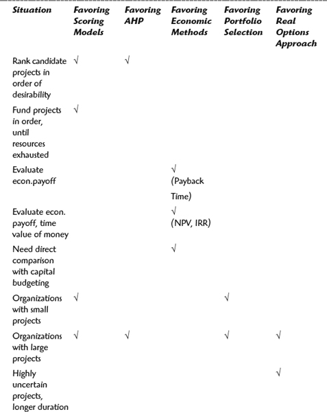
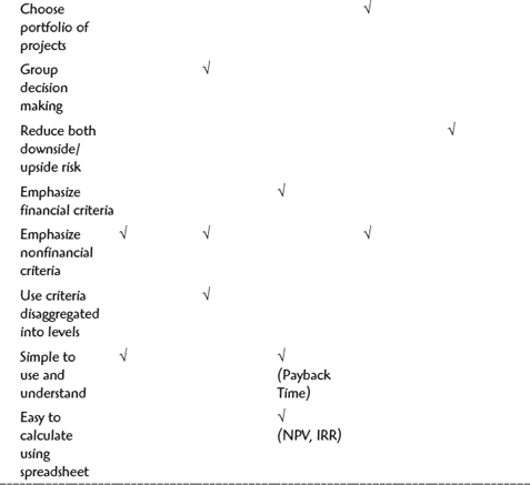
References
1. Cooper, R. G., S. J. Edgett, and E. J. Kleinschmidt. 1998. “Best Practices for Managing R&D Portfolios: Lessons from the Leaders-II.” Research Technology Management 41(4): 20–33.
2. Henrickson, A. D. and A. J. Traynor. 1999. “A Practical Project-Selection Scoring Tool.” IEEE Transactions on Engineering Management 46(2): 158–170.
3. Saaty, T. L. 1983. “Priority Setting in Complex Problems” IEEE Transactions on Engineering Management 30(2): 140–155.
4. Liberatore, M. 1987. “An Extension of the Analytic Hierarchy Procedure for Industrial R&D Project Selection and Resource Allocation” IEEE Transactions on Engineering Management 34(1): 12–21.
5. Saaty, T. L. 1980, The Analytic Hierarchy Process. New York: McGraw-Hill.
6. Kocaoglu, D. F. 1983. “A Participative Approach to Program Evaluation” IEEE Transactions on Engineering Management 30(3): 112–118.
7. Gear, A. E. 1974. “Review of Some Recent Developments in Portfolio Modeling in Applied Research and Development” IEEE Transactions on Engineering Management 21(4): 119–125.
8. Dickenson, M.W., A. C. Thornton, and S. Graves. 2001. “Technology Portfolio Management Optimizing Interdependent Projects over Multiple Time Periods” IEEE Transactions on Engineering Management 48(4): 518–527.
9. Luehrman, T. 1998. “Strategy as a Portfolio of Real Options.” Harvard Business Review. 76(5).