
5 Modeling with UML and Its Real-Time Profiles
Emilia Farcas, Ingolf H. Krüger and Massimiliano Menarini
CONTENTS
5.1.1 Challenges for MBE in Embedded Systems
5.2 Requirements for Modeling Languages
5.3.1 Metamodeling Architecture
5.3.2.1 Requirements Modeling with UML
5.3.2.2 Modeling Logical and Technical Architectures with UML
5.3.4 UML Behavioral Semantics
5.4 UML Extensions for Real Time
5.4.1 Overview of UML Profiles
5.4.2 Modeling and Analysis of Real-Time and Embedded Systems
5.1 Introduction
Embedded systems, such as automotive, avionics, communications, and defense systems, are notoriously difficult to design and develop because of increasing complexity, heterogeneous requirements (combining, e.g., noncritical infotainment and hard real-time engine control), distributed infrastructure, distributed development and outsourcing, time to market, lifecycle management, and cost, to name just a few. Model-based engineering (MBE) [1] greatly contributes to the development of dependable systems with models playing an important role in domain analysis, requirements elicitation, architecture specification, analysis, documentation, and evolution. Nevertheless, while modeling is accepted as a key engineering activity especially in all engineering disciplines outside of software engineering, it is often seen as standing in the way of “the code,” and if it is used, it is often only for forward engineering (i.e., creating code from specifications), leaving activities such as diagnosis and failure management to be addressed separately.
The Unified Modeling LanguageTM (UML®) [2,3] is a general-purpose modeling language—a standard managed by the Object Management Group® (OMG®)—widely used in both academia and industry. It is a family of graphical notations underpinned by a single metamodel [4]. UML can be used at different levels of the development process, especially for requirement modeling and functional design, resulting in specification for behavior, structure, and quality of service (QoS) properties. There exist several UML compliant modeling tools that support code generation to C/C++, Java, Ada, different Real-Time Operating Systems (RTOSs), and Common Object Request Broker Architecture (CORBA®). Moreover, through its profile mechanism, UML can be tailored for various domains or different target platforms.
In this chapter, we present the modeling capabilities of UML and its extensions for real-time systems. We are not providing an introductory UML tutorial, but instead we assume that the reader is familiar with most basic UML notations. Furthermore, we discuss requirements for modeling languages, which helps us pinpoint how and to what degree UML can be used for modeling aspects of real-time systems. This also allows us to identify open issues, such as model consistency, that remain to be addressed to provide a systematic modeling methodology.
In the following paragraphs, we discuss the challenges in embedded systems and how models can be used in various steps in the development process.
5.1.1 Challenges for MBE in Embedded Systems
Embedded systems are often developed by integrating components that have been designed and implemented by different teams, often specialized in different disciplines such as mechanical, electronics, and software engineering. As the system behavior emerges from the interplay of multiple distributed components, a key challenge is the correct integration of all these components. System integration is often performed in vertical design chains such as in automotive and avionics, and the development chain typically involves several tools that are not integrated, as explained below.
For example, embedded systems in automobiles are developed as a joint engineering process between an original equipment manufacturer (OEM) and suppliers. The car manufacturer or OEM traditionally specifies the requirements of the various electronic control units (ECUs) for the car. Each ECU is produced by (external) companies known as suppliers. The OEM then integrates the supplier’s components into the vehicle. Achieving independent component development by suppliers necessitates precise and expressive requirements and interface specifications, as well as an integration framework that addresses quality requirements that crosscut multiple components. In practice, requirements are seldom expressed precisely enough, and system integration has to consider the effects of interactions among distributed components. Therefore, projects often use joint iterative development between the OEM and suppliers to ensure corrective feedback cycles.
Furthermore, the specification and implementation of diagnostic functions, for example, is often implemented ad hoc based on a stream of documents exchanged between the OEM and the suppliers. In the automotive domain, model-based approaches leveraging tools such as MATLAB® [5] and Simulink® [6] from MathWorks and ASCET® [7] from ETAS are used to model control functions and generate implementations for different platforms. However, in practice, there is no formal model of diagnosis that is exchanged between parties. Consequently, it is impossible to validate the design and anticipate problems in putting together the various components in the later phases of the development. The lack of an integrated diagnostic model also limits the reuse of diagnostics across models and generations of cars. Redeveloping diagnostic functions, obviously, leads to higher cost in all areas of requirements engineering, design, development, maintenance, verification, and validation.
Models and MBE hold promise for overcoming these exemplar challenges. Models should serve as a common interface between requirements and architecture specification—using models is the only systematic way to ensure that parties can communicate across all development phases from requirements to acceptance tests. The ultimate goal of MBE is that engineers will spend most of their time modeling the system under consideration and then generate code for a specific target platform. This goal is already supported by various tools (including MATLAB and Simulink), but the models often do not include all aspects of the system, as explained earlier. When automatic code generation is not feasible at the level of the entire system, there is still significant benefit if modeling is used for requirements gathering and architecture verification before deploying the actual system. Various terms are used in the literature to denote the use of models in the development process (e.g., Model-Driven Architecture® [8], model-based design [9], model-driven engineering [10], and model-integrated computing [11,12]). We use the general term MBE as a super-set for all model-based approaches.
In the past decade, significant advances in the area of model specification, transformation, analysis, and synthesis have brought the vision of MBE within reach. Challenges for a comprehensive methodology include providing modeling techniques that result in a consistent, integrated specification; models expressive enough to support both generic and domain-specific aspects of the system; model reusability and integration; model execution; and seamless tool suites.
5.1.2 MBE Process
In general, Fowler [13] identified three ways of using models (specifically, models in UML): sketch, blueprint, and programming language. In sketching, models are used to communicate some aspects of the system. As blueprints, the models should be sufficiently complete as to allow straightforward implementation. By using a modeling language as a programming language, the system is specified at the level of models, and then tools are used to automatically generate the code for the target platform.
In the case of embedded systems, sketches are useful for requirements elicitation because each requirement addresses only a partial view of the system and, thus, a model for an individual requirement is by definition an incomplete specification. Moreover, in the early phases of system engineering, rarely all requirements, let alone their interplay, are understood. On the one hand, sketches as an early analysis tool are generally not hampered by lack of precision in the modeling language proper. To use a model as a blueprint or a programming language, on the other hand, requires the precise specification of the platform and the environment in which the system will operate. Blueprints for embedded systems can support system verification before deploying the actual system, and such verification should include timing requirements, resource usage, and other characteristics of embedded systems. Using a model as a programming language requires powerful tools for code synthesis. Sometimes, code generated from models (e.g., MATLAB and Simulink) is manually adjusted to meet the timing constraints, in which case the link between the code and the model is lost. Moreover, topics such as system reconfiguration and diagnosis are difficult to address. Therefore, a comprehensive MBE approach should involve round-trip engineering.
Figure 5.1 shows a simplified view of the activities and models involved in an MBE process. We use the terms logical architecture and technical architecture as described in Pretschner et al. [14]. The logical architecture is the decomposition of the system into functional components independent of the platform that will execute them, whereas the technical architecture specifies the representation of the logical components in terms of platform-specific entities. A logical architecture can be mapped to multiple technical architectures, each capturing all aspects of a particular deployment. Various other terms are used in the literature to distinguish between logical and technical system aspects. For example, OMG’s Model-Driven Architecture® (MDA®) [8] distinguishes between a platform-independent model (PIM) and a platform-specific model (PSM). Furthermore, the Department of Defense Architecture Framework [15] distinguishes between operational views and systems views to separate the logical and technical architectures. We maintain the use of logical and technical architecture to encompass both these standards.
The modeling process involves creating and refining abstractions in a series of steps. Starting with requirements, we first construct requirements models. Next, we construct logical architecture models, which show how the system achieves the functionality described in the requirements models. At the same time, we use the requirements analysis to select and model a deployment and execution platform. Next, we map the logical models onto the platform, thereby obtaining a technical architecture.
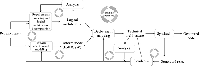
FIGURE 5.1 Simplified model-based engineering process.
Analysis and simulation can be performed at various levels. Logical models can be analyzed for consistency and correctness, whereas technical models can be analyzed for realizability of the deployed system (e.g., schedulability analysis).
The modeling process involves feedback loops, and multiple iterations are possible in each step, within sequences of steps and within the entire process from the beginning. For example, analyzing the technical architecture can reveal hidden requirements and, therefore, may lead to reiterating the process from the initial phase of requirements modeling. We emphasize the need for an iterative process in alignment with the spiral [16] model of agile development methodologies, where requirements often resolve to partial specifications and refinements at one stage can trigger iterations at some earlier stages. An iterative process also accommodates architectural spiking, which is defined as taking a partial set of requirements/use cases and generating a system architecture and implementation based on them, then adding more and more use cases over subsequent rounds. Architectural spikes help in identifying the most critical parts of the system and implementing them first to verify that they can be addressed as expected and, therefore, to mitigate the risks associated with them.
5.1.3 Outline
In the preceding paragraphs, we presented the modeling process in general and various ways of using models, with the implications in the case of embedded systems. We also discussed the current state of the art and challenges in MBE.
The remainder of the chapter is structured as follows. In Section 5.2, we identify requirements for a comprehensive modeling language for embedded systems. This allows us to better position UML’s capabilities in response to this requirements spectrum. In Section 5.3, we present an overview of UML, its metamodeling architecture, extension mechanism, and behavior semantics. We also show how UML can be used for modeling real-time systems, by means of a simplified example from the Bay Area Rapid Transit (BART) [17] system. In Section 5.4, we provide an overview of UML profiles relevant for real-time systems and we cover more detailed aspects from the UML profile for Modeling and Analysis of Real-Time and Embedded systems (MARTE) [18]. In Section 5.5, we discuss how the UML and MARTE together meet the requirements presented in Section 5.2.
5.2 Requirements for Modeling Languages
In the following, we present a set of requirements that modeling languages should meet for a comprehensive methodology of real-time systems. We have identified these requirements based on our experience in several automotive projects with industry partners. The list is not intended to be exhaustive, as further requirements have been presented elsewhere (e.g., Gerard et al. [19]). We focus our presentation on the specification capabilities of a modeling language and not on the entire end-to-end MBE approach nor on the tools necessary to implement it.
Consistency. A modeling language should allow grouping of requirements, structure, behavior, and analysis in a single, integrated system model. Therefore, the language should allow consistency checking for models expressed in different notations, developed in different design iterations, or models that are part of different views/slices of the same system.
Traceability. Requirements should be mappable to a precise specification of the system and from there to implementation while the mapping should be kept current during the system evolution. Traceability also applies to models at different levels of abstraction, enabling conformance checking for refinement operations.
Realizability. Models often represent partial specifications that are refined in successive iterations in the development cycle. Models also represent different views on the system. The underlying question is whether the models allow a system to be constructed such that all requirements are fulfilled. At the very least, we would like to know which requirements stand in the way of realizability.
Distribution and integration. System behavior emerges as the interplay of the functionality provided by subsystems, often developed independently by different suppliers. Thus, models should be capable of expressing concurrency and synchronization. Furthermore, since the OEM is responsible for the integration of subsystems, modeling should support overarching system specification, addressing the integration requirements as well as concerns that cut across the individual components such as resource optimization across the integrated system.
Interdisciplinary domains. Embedded systems design involves multiple domains such as mechanical, electronics, and software. The system components are often designed at different stages in the development process, by different teams, using different tools and languages. A common modeling language should ease integration and tradeoff analysis, and it should reduce the need for disruptive feedback iteration cycles.
Nonfunctional properties. A modeling language should allow specifying nonfunctional properties (such as performance, reliability, and power consumption) associated with behaviors, refinement relationships, deployment models, etc. Moreover, the set of nonfunctional properties should not be predefined and the language should support the specification of application-specific properties.
Resource models. Embedded systems interact with the physical world and are constrained by the resources provided by the hardware and software platforms. Therefore, a specification should support modeling of platforms and resources, as well as allocation and optimization of resources to meet the functional and nonfunctional requirements.
Timing. Time plays a critical role in real-time systems and, therefore, a modeling notation should express timing requirements in various temporal models: (i) causal models, which are concerned only with the order of activities, (ii) synchronous models, which use the concept of simultaneity of events at discrete time instants, (iii) real-time scheduled models, which take physical durations and the timing of activities as influenced by central processing unit (CPU) speed, scheduler, utilization, etc., into account, and (iv) logical time models (e.g., Giotto [20, 21 and 22] and TDL [23,24]), which consider that activities take a fixed logical amount of time, assuming that the platform can execute all activities to meet their constraints.
Heterogeneous models of computation and communication. Real-time systems are often embedded systems that control physical processes, which are often represented in terms of mathematical models. A modeling specification should support continuous behaviors, discrete event-based or time-based behaviors, or combinations thereof.
In the following sections, we present an overview of modeling with UML and its profiles. In Section 5.5, we revisit the requirements identified above and identify open issues in UML.
5.3 Modeling with UML
UML is a family of graphical notations that support modeling structural (i.e., static) and behavioral (i.e., dynamic) views of a system. Among others, the structural view includes class and component diagrams, while the behavior view includes sequence and state machine diagrams. UML provides 14 types of diagrams, though some are used more often and more prominently than others—a guide to the key aspects of the UML can be found in Fowler [13]. In this chapter, we focus on some of the commonly used diagrams.
UML was created to unify many object-oriented graphical modeling notations that became popular in the early 1990s. UML appeared in 1997 and underwent several changes from one version to another, the most radical ones taking place with the transition to UML 2. The most recent version is UML 2.3, whose specification consists of the UML Superstructure [3] defining the notation and semantics for diagrams and the UML Infrastructure [2] defining the language on which the superstructure is based.
In this section, we discuss the metamodeling architecture, the basic modeling capabilities of UML, the extension mechanisms, and behavioral semantics of UML. Then, in Section 5.4, we present an overview of the profiles for real-time systems and go into the details of the MARTE profile. In the end, we discuss the advantages and open issues in UML with respect to the requirements for modeling languages identified in Section 5.2.
5.3.1 Metamodeling Architecture
All graphical notations in UML are backed by a single metamodel. The notation (e.g., a class diagram notation) is the graphical syntax of the language. The metamodel defines the concepts of the language—the abstract syntax. Therefore, the UML metamodel defines the language elements and the relationship between them in the different UML graphical notations (e.g., sequence diagrams and class diagrams). A modeler who uses UML diagrams only as sketches is typically not concerned that much with the metamodel. However, for blueprints and especially for using UML as a programming language [13], the metamodel is very important.
The metalayer hierarchy for any language generally has three layers: (i) the metamodel, or the language specification, (ii) the model, and (iii) objects of the model. The metamodel defines how model elements in a model are instantiated. This layered structure can be applied recursively, such that the same layer that is a model instantiated from a metamodel can be seen as a metamodel of another model at the next lower level of instantiation.
The OMG has developed a modeling language (similar to a class diagram) called the Meta Object Facility (MOFTM) [25], which is used to specify metamodels, such as the UML metamodel. From the perspective of MOF, the UML metamodel is seen as a user model that is based on the MOF metamodel. Therefore, MOF is commonly referred to as a meta-metamodel.
Figure 5.2 shows the four-layer metamodeling architecture used by the OMG: meta-metamodel (layer M3), metamodel (layer M2), model (layer M1), and the run-time system (layer M0). The top layer (M3) provides the meta-metamodel (MOF) that is used to build metamodels. The UML metamodel (layer M2) is an instance of the MOF. Layer M1 models are user models written in UML, and these models are instances of the UML metamodel. The M0 layer contains the runtime instances of the model instances defined in layer M1. The layers are numbered from M0 upward, but the architecture is not restricted to four layers. In general, more layers can be used by applying the recursive pattern as explained before.
Figure 5.2 also shows an example, where the meta-metaclass Class is defined as part of MOF. Then, UML defines the metaclasses Class and Attribute as part of the UML metamodel. Every model element in UML is an instance of exactly one model element in MOF. The UML Class is instantiated in a user model in a class called Train, with an attribute called Speed. Layer M0 contains an instance of a Train.
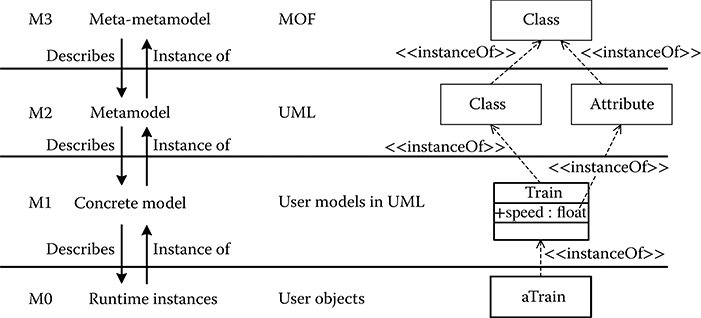
FIGURE 5.2 Metamodeling architecture.
The UML Infrastructure [2] defines a common package Core such that model elements are shared between UML and MOF. UML is defined as a model based on MOF used as metamodel; however, both UML and MOF depend on Core. Therefore, Core can be seen as the architectural kernel, and the Infrastructure defines the foundations for both M2 and M3 layers. The Superstructure [3] extends and customizes the Infrastructure to provide the modeling elements of UML.
5.3.2 Modeling with UML
In this section, we start with presenting the UML diagrams briefly, then we comment how they can be used for modeling requirements and architectures, and in the end we present a modeling example with the basic capabilities.
Figure 5.3 shows the types of diagrams provided by UML for modeling structure and behavior. A UML model consists of elements such as packages, classes, and associations. UML diagrams are graphical representations of a UML model. Examples of using UML diagrams for real-time systems are available in Douglass [26, 27 and 28].
Structure diagrams show the static structure of the system at different abstraction levels and how system elements relate to each other. Class diagrams show system Classifiers such as classes and interfaces, their attributes, and relationships between them. Object diagrams show instances of Classifiers and instances of associations between them. Composite structure diagrams show the internal structure of a Classifier. Component diagrams show logical or physical components and dependencies between them via required and provided interfaces. Package diagrams show packages (i.e., namespaces used to group together elements that are related) and dependencies between them. Deployment diagrams show the assignment of software artifacts to execution nodes. A component may be implemented by one or more artifacts.
Behavior diagrams show the dynamic behavior of the system objects over time. Use case diagrams show a set of actions that some actors perform. Activity diagrams show sequences and conditions for coordinating lower-level behaviors. State machine diagrams model the behavior of a part of the system through finite state transitions. Sequence diagrams show the messages exchanged between entities. Communication diagrams show the interaction between entities, where the sequence of messages is given as a sequence numbering scheme. Interaction overview diagrams are similar to activity diagrams but focus on the overview of the control flow. Timing diagrams show interactions and conditions along a linear time axis.
Some diagram types blur the boundary between structure and behavior. For instance, sequence and object diagrams display aspects of both. Figure 5.3 classifies the diagrams according to their dominant trait.
5.3.2.1 Requirements Modeling with UML
For requirements engineering, modelers first create domain models to describe the existing system for which the software should be built, capturing domain entities and their structural and behavioral relationships in a systematic way. Domain models cover stakeholders, human actors that interact with the system, hardware devices, and the environment in which the system will operate. UML class diagrams can be used for specifying structural domain model aspects, showing the relationships between system entities. UML class diagrams can also be used to specify business rules implicitly through class composition and multiplicity constraints, as well as explicitly through pre- and post-conditions expressed in Object Constraint Language (OCL) [29]. Such domain models can help in defining the questions for stakeholders and uncovering hidden requirements. Models also help in defining the boundaries between the target system and its environment.
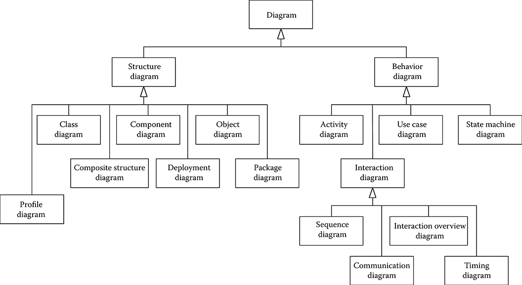
FIGURE 5.3 Unified Modeling Language structure and behavior diagrams. (From Object Management Group, “Unified Modeling Language (OMG UML), Superstructure, Version 2.3,” formal/2010-05-05, OMG, 2010. With permission.)
UML use case diagrams identify actors and the capabilities of the system. Use cases are useful also in eliciting end-to-end timing and other QoS requirements, often expressed as constraints of the form “when the actor does X, the system should respond within Y ms.”
The next level of detail beyond use cases is often a set of scenarios that depict interactions between the actors of the use case when using that specific capability of the system. Scenarios are modeled as sequence diagrams, capturing the operations performed by the system, the message protocol of interaction between the system and its actors, and constraints. UML activity and communication diagrams (previously called collaboration diagrams) can also be used to show how actors collaborate to perform tasks.
5.3.2.2 Modeling Logical and Technical Architectures with Uml
After identifying requirements, architecture and design models show how the system is structured and how its internal entities behave to achieve system goals. All diagrams from Figure 5.3 can be used at this stage. In general, a type of structural or behavioral diagram can be used both for the logical and technical architecture. The models relevant to the logical architecture focus on capabilities and their mapping to logical entities, whereas the models relevant to the technical architecture focus on deployment entities. A platform model adds details such as middleware, operating system, network, and resources. The technical architecture then expresses the mapping between the logical architecture and the platform. In particular, package and deployment diagrams are used for the technical architecture. Furthermore, UML profiles such as MARTE [18] support the modeling of software and hardware resources in a standard way (see Section 5.4).
UML is the language choice of MDA, where both PIM and PSM are expressed as UML models. Model transformation from PIM to PSM is a core concern of MDA, and a PIM has to contain sufficient detail for a tool to generate a PSM. In MDA, the PSM contains the same information as an implementation, but in the form of a UML model instead of code. In general, UML is often used for modeling the logical architecture and other languages can be used for the technical architecture. However, if the transformation is not performed automatically or if it cannot be formalized, then the traceability between the logical and technical architecture is lost.
As concurrency and timing constraints are of particular concern in real-time systems, in the following, we discuss how UML supports them. Concurrency can be modeled in communication diagrams via the sequencing mechanism for events. Messages with the same sequence numbers (e.g., two messages numbered 3a and 3b) can be simultaneously triggered, provided that all messages with lower sequence numbers have been successfully triggered. Furthermore, concurrency can be expressed in sequence diagrams via the interaction operator PAR, which expresses parallel execution of a set of operations.
The Simple Time package defined in the UML Superstructure [3] provides basic support to represent time and durations and to define timing constraints. A time event denotes an absolute or relative point in time (relative to the occurrence of other events) when the event occurs. A time event is specified by an expression, which may reference observations. A time observation denotes a time instant to be observed during execution when a model element is entered or exited. A duration observation denotes an interval of time. For example, a time constraint can be associated with the reception of a message. In UML, timing constraints can be used in sequence diagrams or state machine diagrams. Simple Time enables triggering a transition in a state machine when a specific point in time has reached or after a certain amount of time has passed. However, the simple model of time does not account for multiple clocks or phenomena such as clock drifts, which occur in distributed systems, leaving more sophisticated models of time to be provided by profiles. In Section 5.4.2, we discuss in more detail how timing constraints are supported in the MARTE profile.
UML also introduces timing diagrams to show the effects of message/event interactions between entities over time. Timing diagrams are useful to depict different states of entities over time, especially in systems with continuous behavior relative to time, but sequence diagrams are more useful in actually modeling explicit time constraints.
5.3.2.3 Uml Basics By Example
To show the modeling capabilities of UML, we use a simplified example of the BART system, particularly the part of the train system that controls speed and acceleration of the trains. BART is the commuter rail train system in the San Francisco Bay area. A full description of the case study is beyond the scope of this chapter, so we will exemplify some of the UML diagrams that can be used for modeling such a system—use case, class, sequence, and state machine diagrams. We will revisit the example in Section 5.4.2.3 when discussing additional capabilities introduced in MARTE and the issue of consistency in UML models.
The BART system automatically controls over 50 trains, most of them consisting of 10 cars. Tracks are unidirectional and sections of the track network are shared by trains of different lines. A track is partitioned into track segments, which may be bounded by gates. A gate can be viewed as a traffic light, establishing the right-of-way where tracks join at switches. Figure 5.4 depicts a domain model for the BART track system, showing in a UML class diagram the relationships between physical entities such as train, track, and gate. Such models facilitate establishing a common language for eliciting requirements from domain experts. Typically, specifying relationships and multiplicity constraints on a domain model leads to further discussions with the stakeholders to clarify the domain. For example, gates are not necessarily associated with switches, but can be used just to control the traffic flow.
Other work [17] describes the Advanced Automatic Train Control (AATC) system, which controls the train movement for BART. One important AATC requirement is to optimize train speeds and the spacing between the trains to increase throughput on the congested parts of the network, while constantly ensuring train safety. The specification strictly defines certain safety conditions that must never be violated, such as “a train must never enter a segment closed by a gate,” or “the distance between trains must always exceed the safe stopping distance of the following train under any circumstances.”
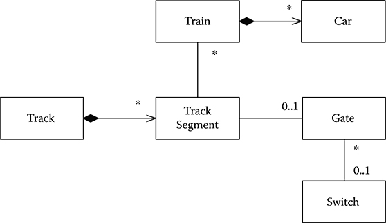
FIGURE 5.4 Class diagram: domain model for the Bay Area Rapid Transit tracks.
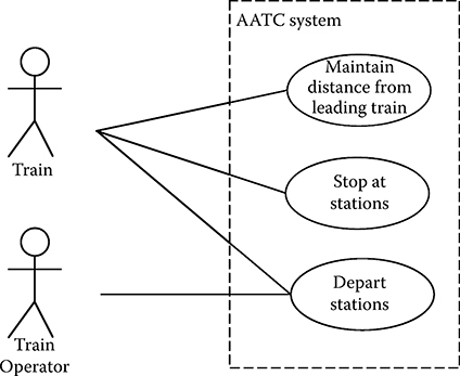
FIGURE 5.5 Use case diagram.
The system is controlled automatically. Onboard operators have limited responsibility: they signal the system when the platforms are clear, so a train can depart a station and they can operate the trains manually when a problem arises. Use case diagrams are useful in identifying the system boundaries (the control system that must be designed) and the external actors that interact with the system. Typically in UML, actors are human actors that use an application, but in embedded systems actors can be external physical resources such as devices and sensors. Nevertheless, actors represent logical roles, so a physical resource could play several roles in UML models. Figure 5.5 depicts a simple use case diagram for BART. Actors that interact with the AATC system are the Train and the Train Operator and so they are part of the system environment. The use cases depict the high-level goals of the system without details on how these goals are accomplished.
AATC consists of computers at train stations, a radio communications network that links the stations with the trains, and two AATC controllers on board of each train—the two controllers are at the front and back of the train. A track is not a loop. Thus, at the end of the line, the front and back controllers exchange roles and the train moves in the other direction. Each station controls a local part of the track network. Stations communicate with the neighboring stations using land-based network links. Trains receive acceleration and brake commands from the station computers via the radio communication network. The train AATC controller (from the lead car) is responsible for operating the brakes and motors of all cars in the train. The radio network has the capability of providing ranging information (from wayside radios to train radios and back) that allows the system to track train positions.
The system operates in half a second cycles. In each cycle, the station control computer receives train information, computes commands for all trains under its control, and forwards these commands to the train controllers. Figure 5.6 shows a sequence diagram depicting the interactions between three roles called Train, Station AATC, and Train Controller. Note that the Station AATC system obtains the status information directly from the Train by using the radio network, not from the Train Controller.
The sequence diagram features interaction frames, introduced in UML 2.0. A frame provides the boundary of a diagram and a place to show the diagram label (e.g., “Control Train Speed” in Figure 5.6). Frames also allow specifying combined fragments with operators and guards. Common examples of operators are LOOP for repetitive sequences, ALT for mutually exclusive fragments, and PAR for parallel execution of fragments. Figure 5.6 uses a LOOP operator to show that the system repeats the sequence of checking the train position and issuing new commands. Another operator is REF, which creates a reference to an interaction specified in another diagram. This REF operator allows composing primitive sequence diagrams into complex sequence diagrams. The expressiveness of UML 2 increased with the addition of these operators, which are borrowed from Message Sequence Charts [30,31].
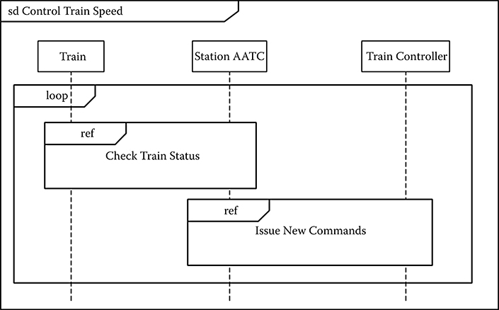
FIGURE 5.6 Sequence diagram that composes two other sequence diagrams.
Figure 5.7 depicts a simplified Check Train Status sequence diagram as referenced in Figure 5.6. The Train sends status information regarding its speed, acceleration, and range. The Station AATC system computes the train position from the status information and updates its Environmental Model. Status messages and commands are time-stamped in the so-called Message Origination Time Tag (MOTT). When a Train sends status information to a station, it attaches the time it sends the message as a MOTT. When the Station AATC estimates the train position, it attaches the original MOTT to the estimate. Furthermore, when the Station AATC sends a command, it again attaches the original MOTT, and the Train Controller checks the MOTT before executing the command. The station’s control algorithm takes the MOTT, track information, and train status into account to compute new commands that never violate the safety conditions. To ensure this, each station computer is attached to an independent safety control computer that validates all computed commands for conformance with the safety conditions.
The actors in sequence diagrams (e.g., Train, Station AATC, etc.) are logical roles—in modeling the interactions, we concentrate on specific use cases and abstract from any concrete deployment architectures. In essence, a role shows part of the behavior the system displays during execution. What concrete deployment entity plays this role is left for a later modeling stage. The natural modeling entities for roles in the UML are Classifiers—with the understanding that multiple roles may be aggregated into a single Classifier. The roles related to computing commands and safety are omitted from Figure 5.7, as they are relevant for another sequence diagram, called Issue New Commands, shown later in this chapter in Figure 5.17. The roles visible in a sequence diagram are a subset of the roles of the entire system.
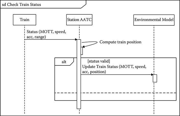
FIGURE 5.7 Sequence diagram for Check Train Status.
Figure 5.8 shows a simplified domain model with the roles mentioned so far. We use the notation of a class diagram without the multiplicities—for a role domain model, we are interested in the roles that communicate and the links between them. The same diagram can be seen as a simplified Communication diagram, showing the communication links without the messages being exchanged. The role domain model is part of the logical architecture, as roles are logical entities that are later mapped onto physical components to define the technical architecture. A component can play several logical roles.
If a train does not receive a valid command within 2 s of the time stamp contained in the MOTT accompanying the status, it goes into emergency braking. Figure 5.9 shows the behavior of the Train Controller as a state-machine diagram with two states for normal operation and emergency mode.
In state-machine diagrams, we show states as boxes with rounded corners. Arrows denote state transitions. Labels on arrows indicate (i) the trigger (such as a message received), (ii) a guard (a condition that must be true for the transition to be taken) in square brackets, separated from (iii) the action (to be performed when the transition is taken) by a “/.” Actions include assignments to state variables and the sending of messages. All three pasts of a transition are optional. A solid circle indicates the initial “pseudo” state.
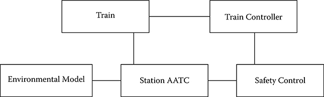
FIGURE 5.8 Role domain model as a class diagram.
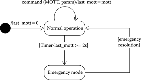
FIGURE 5.9 State-machine diagram for Train Controller.
This example shows a frequently used pattern in modeling time with the basic capabilities of the UML: time is represented as an explicit parameter in messages exchanged among actors and these actors then perform explicit time arithmetic to determine transition triggers.
5.3.3 UML Extension Mechanism
The UML standard supports two types of extension mechanisms: lightweight extension through profiles and first-class extension through MOF. The profile mechanism allows UML metaclasses to be specialized for specific domains or different target platforms. In profiles, it is not possible to modify existing metamodels or to insert new metaclasses. Thus, in profiles it is impossible to remove constraints that apply to the UML metamodel, but it is possible to add new constraints that are specific to the profile. In contrast to profiles, in first-class extensibility, there are no restrictions on what changes can be made to a metamodel as MOF enables adding new metaclasses, removing existing classes, and changing relationships. In other words, the profile’s extension defines a new dialect of UML, whereas the first-class extension defines a new language related to the UML.
Stereotypes, tagged values, and constraints are the main extension mechanisms available in a profile. A profile extends a reference metamodel such that the specialized semantics do not contradict the semantics of the metamodel. As such, the reference model is considered “read only.” Stereotypes allow creating new model elements (not new metamodels), new constructs specific to a particular domain or platform. As such, a stereotype extends an existing metaclass and uses the same graphical notation as a class, with the keyword «stereotype» shown before or above the name of the stereotype. When the stereotype is applied to a model element, the name of the stereotype is given between «». A metaclass is extended by a stereotype by using a special kind of association relationship called an extension, which supports flexible addition/removal of stereotypes to classes. The notation for an extension is an arrow pointing to the extended class with the arrowhead as a solid triangle.
For example, for real-time systems, the MARTE profile defines the stereotype «RtUnit» to denote a real-time processing unit as shown in Figure 5.10. The left-hand part of the figure shows the stereotype definition (the stereotype extends the metaclass BehavioredClassifier) and the right-hand part of the figure shows how the stereotype is applied to the model element Train Controller. A stereotype definition must be consistent with the abstract syntax and semantics of UML but can adapt the concrete syntax of UML to the domain. A stereotype can use an icon instead of a UML diagram element as, for example, when defining a clock element.
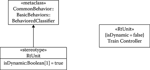
FIGURE 5.10 Stereotype example.
The properties of a stereotype are called tag definitions. When a stereotype is applied to a model element, the values of its properties are called tagged values. Thus, tagged values are defined as tag–value pairs, where the tag represents the property and the value represents the value of the property. In previous versions of UML, tagged values allowed defining additional properties for any type of model element. Starting with UML 2, a tagged value can be represented only as an attribute on a stereotype. For example, Figure 5.10 shows the Boolean attribute isDynamic defined for the stereotype «RtUnit». If this attribute is true, the real-time unit dynamically creates the schedulable resource required to execute its services [18]. When applying the stereotype, tagged values can be shown in the class compartment under the stereotype name as shown in Figure 5.10 for Train Controller. However, tagged values may also be shown in a comment attached to the stereotype.
A profile consists of a package that contains one or more related extension mechanisms. Profile diagrams (see Figure 5.3) allow defining custom stereotypes, tagged values, and constraints. Constraints allow extending the semantics of the UML metamodel by adding new rules. Constraints can be specified in OCL (not shown here for reasons of brevity).
Compared to pure stereotyping, the advantage of using the UML profile mechanism is that UML’s meta- and meta-metamodels provide a shared semantic and syntactic foundation across all profiles.
5.3.4 UML Behavioral Semantics
UML semantics is a topic that ignites fierce discussions in the modeling community. A common argument of UML critics is that UML has no behavioral semantics. While this was true for the first version of the language, OMG introduced an action-based semantics into the UML version 2.0 standard. Because UML supports expressing behavior in different specialized languages (i.e., state machines and activity diagrams), the semantics defined in the standard uses generic and fine-grained elements, which are composed to support all these sublanguages. UML is also intended to be used in different domains that have diverse execution requirements. Therefore, the UML standard defines variation points for which the documentation states alternative behaviors or leaves explicitly unspecified the behavior, calling for profiles to choose the most appropriate set of behaviors for the intended application domain.
Shortcomings of UML semantics are an important topic of discussion in the modeling community. Some scientists [32] point out that, even if a semantic model exists in the standard, it is not adequate to many usage scenarios. A first criticism is that the semantics is not defined formally, in terms of pure math of other formal languages. Consequently, it is impossible to prove that UML semantics is consistently defined or to develop verification tools that check behavioral properties of UML models. A second criticism is that the standard documents do not contain a chapter that coherently describes UML semantics. In fact, semantics information is spread across the standard and discussed together with the different UML notations. This makes it difficult for the reader to grasp UML semantics and thus paves the way for inconsistencies in the definition and misinterpretation by users. Additional critics complain about the very simple time model, which uses a centralized unique clock and must be completely replaced in many domains. Finally, the variation points that make UML applicable to any domain are subject to criticism as they force adopters to create semantic variations for each such domain.
In the remainder of this section, we describe some of the key elements of UML semantics and how they connect to structural elements of UML. We do not present the semantics of specific UML behavioral notations (e.g., interaction diagrams) but focus on the key elements that are used in the UML standard to construct the semantics of such notations. In our description, we highlight some variation points that are left open for profiles to specify. In Section 5.4.2.2, we discuss how the MARTE profile uses those variation points to create a behavioral semantics amenable to real-time embedded systems.
The first step for understanding UML behavioral semantics is defining how behavior is specified and which elements participate in an instance of such behavior. UML specifies behavior by defining flows of actions. These flows are always attached to a structural element, a Classifier. UML distinguishes between two types of objects with behavior: active and passive. Active objects, on the one hand, are the source of behavior. When created, they execute their actions independently of any other object. Passive objects, on the other hand, execute their actions in reaction to requests from other objects. Active objects subsume familiar programming concepts such as threads of execution and processes. The UML specification uses this more generic representation so that it can include behavior of entities that are not necessarily programs (e.g., people).
Figure 5.11 depicts the subset of the UML metamodel that defines the Behavior class and its connection to Behaviored Classifiers. Behavior is the superclass that represents all behaviors in the UML. Therefore, all the UML notations that describe behavior inherit this basic definition and enrich it by defining more specific types of behavior and their descriptions. Behaviors are associated to BehavioredClassifier. Because the UML Classifiers define sets of instances, the figure shows that behaviors are contained in instances of model elements. This is expressed by the use of a composition relation (black diamond) in the ownedBehavior association of Figure 5.11. The figure also shows that instances can be associated with a classifier Behavior, which represents the behavior that active objects start executing when created.
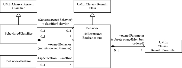
FIGURE 5.11 Subset of common behavior from package BasicBehavior. (From Object Management Group, “Unified Modeling Language (OMG UML), Superstructure, Version 2.3,” formal/2010-05-05, OMG, 2010. With permission.)
The UML standard specifies the behavior performed by Behavior objects in terms of actions and action flows. Actions are elementary operations that, given sets of inputs, produce sets of outputs and optionally modify the value of some structural elements. Multiple actions can be composed into flows to specify more complex operations. Flows specify networks of actions and, as such, identify dependencies between subsequent actions and how outputs feed into subsequent inputs. To support different types of systems requiring diverse semantic choices, UML supports variation points in the action model. One such variation point is the type of dependencies that flows can define. UML has two types of flow dependency: control flow, which starts the dependent action only when the previous one ends, and object flow, which starts dependent actions as soon as all their inputs are available. A second variation point arises by the fact that UML does not mandate when the elements of the action output sets become available. Different decisions on when to make the output values available create very different semantics. For example, UML could support semantics that assume synchronous reactions.
Messages and events are the final building blocks that form the base of the UML behavioral semantics. Messages support communication between different instances of UML elements. For example, different message patterns support synchronous calls, asynchronous calls, and signal broadcast. Messages are received in message pools and presented to the receiving instances when they are ready to receive. What happens to an incoming message when the pool is full and in which order messages in the pool are presented to the receiving instance are semantic variation points. Reception of messages is an example of an event. UML events represent the occurrence of a generic state or condition in the UML model instance. Types of events include call events, expression change events, and time events. Some events act as triggers, in which case a Behavior starts executing when the event occurs. Other events just capture a state. For example, a send signal does not even initiate a new behavior whereas a receive signal may.
A very good summary of the UML 2.0 semantics is provided by Selic [33]. We also suggest the interested reader to consult the standard documents [2,3], in particular, to understand how the UML behavior notations (Sequence Diagrams, State Machines Diagrams, Activity Diagrams, etc.) use the core elements we discussed to concretely define their semantics.
5.4 UML Extensions for Real Time
In this section, we discuss various extensions of UML and then show details from the recent profile for MARTE. The extension mechanism in UML (see Section 5.3.3) allows the definition of families of languages targeted to specific domains and levels of abstractions.
5.4.1 Overview of UML Profiles
The profile mechanism has been specifically defined for providing a lightweight extension mechanism to the UML standard via stereotypes, tagged values, and constraints as described in Section 5.3.3. For example, other work [34] presents a UML profile for a platform-based approach to embedded software development using stereotypes to represent platform services and resources that can be assembled together. There is an increasing number of profiles defined in various domains, resulting from either OMG standardization efforts or research outcomes. Different profiles may be overlapping and also inconsistent as each profile tailors the UML for a particular domain or platform. Some of the profiles emerged in previous versions of UML and then new profiles were defined to keep up with the latest changes in UML and to fill in the gaps identified in practice. In the following, we discuss some of the most commonly used profiles for real-time systems, with the historical background and the relationships between them.
The profile mechanism has been significantly refined starting with UML 2.0. Initially, UML 1.0/1.1 provided stereotypes and tagged values, but did not define the concept of a profile. Subsequent revisions of UML introduced the concept of a profile to provide structure to the extension elements. Moreover, to complete the previous versions of UML, the UML 2.0 Infrastructure and Superstructure specifications have defined the profile mechanism as a specific metamodeling technique. In addition, profile diagrams have been introduced in UML 2.0.
UML/Realtime (UML-RT) [35,36] extended UML 1.1–1.4 to support Real-Time Object-Oriented Modeling [37] concepts. It was also the UML dialect of the CASE tool Rational Rose®/RT. The extension used the standard UML mechanisms of stereotypes, tagged values, and constraints. Thus, UML-RT is a profile, although it was not called a profile initially because there was no profile concept in UML 1.1. For modeling architectural concepts, UML-RT introduced capsules (to model components), ports (to model the interaction of a capsule with its environment), connectors (communication channels between ports), and protocols (to model the behavior that can occur over a connector). A protocol comprises a set of participants (protocol roles), each specified by a set of signals received/sent by it. The corresponding communication sequence can be specified by a state machine and sequence diagrams. While UML-RT was a substantial improvement over the first generation of UML to model real-time systems, it still did not support all notations needed in modeling real-time systems. For example, Krüger et al. [38] presents an extension to UML-RT to support broadcasting. Because UML-RT was not based on an extensible framework such as the one supported by UML 2.0, extending it was an ad hoc process. UML-RT concepts were finally included in UML 2.0, which grants not only the ability to use its constructs in standard UML, but also the ability to systematically extend such constructs. For example, Krüger et al. [39] presents an approach to introducing broadcasting using UML 2.0 facilities similar to the UML-RT approach we mentioned earlier [38].
The UML profiles standardized by OMG include the UML Profile for Schedulability, Performance, and Time (SPT) [40], the UML profile for MARTE [18], and the UML profile for QoS and Fault Tolerance (QoS & FT) [41]. UML-RT focused on component-oriented development of communicating systems but left other aspects of embedded systems unaddressed. The SPT profile [40] was developed to define a resource model, time, and concurrency aspects in UML. MARTE is a new UML profile that updates the previous profile SPT for UML 2.x. MARTE is presented in more detail in Section 5.4.2. The QoS & FT profile [41] defines resource properties such as memory capacity and power consumption. The QoS & FT profile allows users to customize service characteristics (i.e., define new characteristics through specialization) and use tools to perform analyses such as performance and dependability. The QoS & FT profile allows defining a wide variety of QoS properties as compared to the SPT profile, which focused on schedulability and performance. In comparison, MARTE reuses concepts defined in both the SPT and the QoS & FT profile. Moreover, MARTE has the advantage that it allows modelers to attach directly to the design model additional information necessary for various analyses, rather than creating dedicated models for analysis.
OMG also provides the standard for the Systems Modeling Language™ (OMG SysMLTM) [42]. SysML reuses a subset of UML 2 (called UML4SysML) and provides additional extensions to address the concerns for systems engineering applications (called the SysML Profile). Therefore, SysML uses both UML extension mechanisms: the first-class extension via MOF is used to define the UML4SysML subset and then the profile extension mechanism is used not on UML but on UML4SysML. SysML does not use all of the UML diagram types and, thus, it is smaller and easier to learn than UML. In particular, SysML strictly reuses the UML use case, sequence, state machine, and package diagrams. SysML also modifies some of the UML diagrams. The SysML block definition diagram, internal block definition diagram, and activity diagrams extend the UML class diagram, composite structure diagram, and activity diagram, respectively. The SysML “block” is a significant extension in the direction of modeling complex systems. Blocks can be used to decompose the system into individual parts, with dedicated ports for accessing their internals. A block can represent almost any other type of structural entity. Furthermore, SysML allows the description of more general interactions than in software, for example, physical flows such as liquids, energy, or electricity. SysML activity diagrams add support for modeling continuous flows of material, energy, or information. By specifying a continuous rate, the increment of time between tokens approaches zero to simulate continuous flow. Nevertheless, SysML does not extend the time model of UML.
SysML adds two new diagram types: the requirements diagram and the parametric diagram. The requirements diagram captures text-based requirements and the relationships between them—requirements hierarchies and requirements derivation. A requirement can be related to a model element that satisfies or verifies the requirements. Thus, SysML requirements modeling not only supports the process of documenting requirements, but also provides traceability to requirements throughout the design flow. It furthermore provides tabular representations for requirements. Parametric diagrams allow the graphical specification of analytical relationships and constraints on system properties (such as performance and reliability) associated with blocks. Thus, parametric diagrams serve the integration of design models with analysis models.
SysML and MARTE are complementary and could be used together in a common modeling framework [43]. In general, there exist several profiles defined in various domains, and it is not clear how to combine multiple profiles when this is necessary for a particular interdisciplinary application. Therefore, Espinoza et al. [43] presents how SysML and MARTE can be combined and highlights the open issues in terms of convergence between the two profiles. For requirements engineering, SysML provides traceability relations, whereas MARTE provides ways to specify nonfunctional requirements. For system structure, modelers could start with a model specified with SysML blocks and then apply MARTE stereotypes to add additional semantics to these blocks. For system behavior, MARTE adopted the notion of port and flow from SysML, but they have different semantics. Therefore, when combining SysML and MARTE, it is required to define a common consistent semantics. Furthermore, significant differences exist in the specification of quantitative values for analysis (see Espinoza et al. [43] for a detailed analysis of the two profiles).
Even from this short exploration of UML extensions and profiles, it becomes clear that model consistency is a critical aspect of MBE—within and across profiles.
5.4.2 Modeling and Analysis of Real-Time and Embedded Systems
The UML profile for SPT [40] provides a framework for specifying time properties, schedulability analysis (rate monotonic analysis), and performance analysis (queuing theory). MARTE [18] updates SPT for UML 2.x. It allows for modeling of both software and hardware platforms along with their nonfunctional properties. It supports component-based architectures and different computational paradigms, and it allows more extensive performance and schedulability analysis.
In this section, we present an overview of MARTE’s capabilities and we revisit the BART case study introduced in Section 5.3.2.3.
5.4.2.1 MARTE Basics
MARTE [18] is structured as a hierarchy of subprofiles (see the UML package diagram in Figure 5.12) with five foundation profiles and then further extensions used for design or analysis.
The foundation profiles are as follows:
Core Elements define the basic elements used for structural and behavioral modeling. MARTE distinguishes between design-time Classifier elements and runtime instance elements created from the Classifiers. Behaviors are composed of actions and are triggered by events. Behaviors provide context for actions and determine when they execute and what inputs they have. In addition, MARTE supports modeling of operational modes (i.e., modal behavior), which are mutually exclusive at runtime. A mode defines a fragment in the system execution that is characterized by a given configuration when a set of system entities are active and have parameters defined for that mode.
Nonfunctional Properties Modeling (NFP) supports the declaration of nonfunctional properties (such as memory usage and power consumption) as UML data types. The Value Specification Language (VSL) is introduced in MARTE to specify the values of those data types using a textual language for specifying algebraic expressions. An annotated model (see Figure 5.13) contains annotated elements, which are model elements that have attached NFP value annotations for describing nonfunctional aspects (which can differ from one operational mode to another). The annotated model establishes the context for interpreting names used in the value specification. Examples of annotated elements (defined in other MARTE packages) used for performance analysis are step (a unit of execution), scenario (a sequence of steps), resource, and service (offered by a resource or component). A Modeling Concern establishes the ontology of relevant NFPs for a given domain used for the analysis. A domain model such as Figure 5.13 shows the concepts defined in MARTE. Then, a profile diagram defines the profile packages and how the elements of the domain model extend metaclasses of the UML metamodel. As explained in Section 5.3.3, the elements in the domain model are represented in the UML as stereotypes (e.g., the stereotypes «Nfp», «NfpConstraint», «Mode», etc.). However, not every element in the domain model results directly in a stereotype, because some of the domain concepts are abstract.
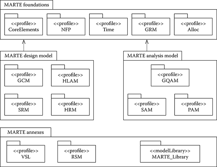
FIGURE 5.12 The architecture of the Modeling and Analysis of Real-Time and Embedded systems (MARTE) profile. (From Object Management Group, “UML Profile for MARTE: Modeling and Analysis of Real-Time Embedded Systems” Version 1.0, formal/2009-11-02, OMG, 2009. With permission.)
The Time profile supports three models of time: chronometric, logical, and synchronous. It enriches the behavior specification from the core elements with explicit references to time concepts. Time is represented as a partial ordering of instants. The occurrence of a time event refers to one instant. The basic model does not refer to physical time and, therefore, supports logical time, which is the basis also for synchronous languages. A time base is a set of instants where MARTE supports discrete and dense time bases (only countable sets). Physical time can be modeled as a dense time base. Clocks (logical or chronometric) use a discrete time base. For distributed systems, multiple time bases are supported.
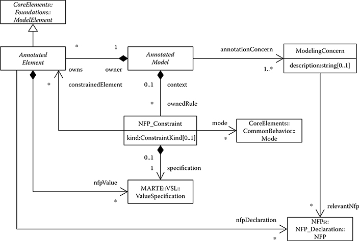
FIGURE 5.13 Nonfunctional properties annotations in MARTE. (From Object Management Group, OMG, 2009, “UML Profile for MARTE: Modeling and Analysis of Real-Time Embedded Systems” Version 1.0, formal/2009-11-02, 2009. With permission.)
Time can be used for triggering behaviors or observing event occurrences. MARTE defines the concepts for relating events, actions, and messages to time. A time constraint is specified as a predicate on timed observations (see Figure 5.14) and so the TimedObservation is a key concept introduced in MARTE. A constraint can be imposed on the occurrence of an event, the temporal distance between two events, or the duration of a behavior execution. A TimedObservation is a TimedElement, and, therefore, it has associated clocks used for observing time. A TimedObservation is the abstract superclass of TimedInstantObservation and TimedDurationObservation. For a behavior, observed events can be either its start or finish event. For a request, the possible events are its send, receive, or consume (the start of its processing by the receiver) events. Duration constraints can be defined on two events not necessarily occurring on the same clock.
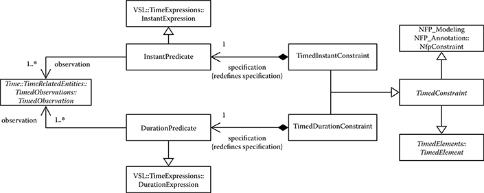
FIGURE 5.14 TimedConstraints as defined in MARTE. (From Object Management Group, “UML Profile for MARTE: Modeling and Analysis of Real-Time Embedded Systems” Version 1.0, formal/2009-11-02, OMG, 2009. With permission.)
Generic Resource Modeling (GRM) provides an ontology of resources that allows the modeling of computing platforms, including computing resources, storage resources, communication media, and execution platforms.
Allocation Modeling (Alloc) provides concepts for allocation of functionality to implementation entities. It includes space allocation and time allocation (i.e., scheduling). It also addresses the issue of refinement between models of different levels of abstraction. Nonfunctional properties (e.g., worst case execution time) can be attached to an allocation specification.
Based on the foundational profiles, MARTE provides two packages of extensions (see Figure 5.12): the MARTE design model supports model-based design of embedded applications and the MARTE analysis model supports model-based analyses and, thus, validation and verification.
For model-based design with MARTE, the High-Level Application Modeling (HLAM) subprofile provides extensions for real-time concerns such as Real-time Unit (using the stereotype «RtUnit») for concurrent computing units and Protected passive Unit («PpUnit») for shared information. An «RtUnit» owns one or several schedulable resources and can satisfy several requests from several real-time units at the same time, enabling intraunit parallelism if necessary. An «RtUnit» owns a single message queue for saving the messages it receives, and each message can be used to trigger the execution of a behavior owned by the unit. Real-time units and protected passive units may provide real-time services, which may specify real-time features such as deadlines and periods (with the ArrivalPattern data type). The stereotype for features («rtf») can be applied to multiple kinds of modeling elements (e.g., actions, messages, and signals). For example, the message Status from Figure 5.7 can be stereotyped as a real-time feature, indicating that is has a period of 500 ms (remember that the AATC system operates in half-second cycles). As a simple example, Figure 5.15 depicts the status message, omitting other messages exchanged in this scenario. We define t0 as a TimedInstantObservation. Because the message is periodic, the period starts at time event t0[i]. Later in the chapter, Figure 5.17 shows an example for specifying timing constraints on the temporal distance between two events.
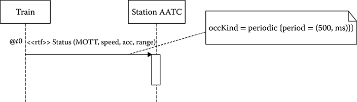
FIGURE 5.15 Bay Area Rapid Transit periodic feature.
The Generic Component Model (GCM) subprofile supports component-based design, with both message and data communication between components. The MARTE component model adopted the concepts of ports and flows from SysML and added client/server ports. Furthermore, Software Resource Modeling (SRM) and Hardware Resource Modeling (HRM) allow designers to specify computing platforms. SRM allows modeling of elements such as tasks, semaphores, mailboxes, etc. The MARTE annexes feature supports modeling of OSEK, ARINC, and POSIX-compliant software computing platforms. The model of computation in MARTE is an asynchronous/event-based approach, but alternative models can be defined as extensions to the MARTE specification by using NFP, Time, and GRM packages.
Model-based analysis with MARTE is provided by the Generic Quantitative Analysis Modeling (GQAM) subprofile or by its two refinement subprofiles for schedulability and performance analysis. The analysis is based on the annotation mechanism in MARTE, which uses UML stereotypes. The model elements are mapped into analysis elements, which include the values for nonfunctional properties necessary for the analysis.
The Architecture Analysis and Design Language (AADL) [44] is an architecture description language defined ab initio (not as a UML profile) and standardized by the Society of Automotive Engineers. A system modeled in AADL consists of application software components (made of data, threads, and process components) bound to execution platform components (processors, memory, buses, and devices). Note that there is a MARTE rendering of AADL, formalized as a subset of MARTE.
5.4.2.2 MARTE Semantics
We discussed in Section 5.3.4 that UML 2.x defines a flexible semantics framework, which leaves several variation points open for profiles to specify. This approach leaves the developers of profiles free to adapt the general framework of UML behavior to the special needs of their target domains. In the case of MARTE, one of the most evident variations is the time model, which we discussed in Section 5.4.2.1. In fact, because the target domain includes real-time systems, the simplistic time model based on a global clock of the UML is not suitable.
While time is the most evident variation over standard UML semantics, MARTE defines semantics for many other variation points that the general UML specification left open. For example, we mentioned in Section 5.3.4 that the order in which messages are removed from the message pool and presented to the receiving instance is an open variation point. MARTE addresses this variation point by defining two default policies (first-in-first-out, FIFO and last-in-first-out, LIFO) and specifying that, by default, messages that arrive when the message pool is full will not be blocking and the message pool will silently drop the oldest message it contains to make room for the new one (see Section 12.3.2.6 in the MARTE profile specification [18]).
A complete discussion of all UML variation points fixed by MARTE is beyond the scope of this chapter. We recommend that the interested reader consult the MARTE profile specification [18] for a complete specification of the MARTE semantics.
5.4.2.3 MARTE Example
In this section, we revisit the BART example introduced in Section 5.3.2.3. We show different modeling perspectives using MARTE, give an example of timing constraints, and present an inconsistency that can arise when modeling behavior in the different diagrams.
Figure 5.16 depicts a component diagram with five components and the interface dependencies between them (we use the graphical notation of a ball-and-socket connection between a provided interface and a required interface). The Environmental Model component models the physical environment containing the trains. The Station AATC uses the Environmental Model to compute commands to send to trains. The Safety Control component checks all commands sent by the Station AATC for safety before forwarding them to each train. The safety computation is based on a simpler model than the one used to compute commands and only focuses on ensuring that all commands sent maintain the safety of each train. The last two components are deployed on the actual train. The Train Controller manages the train accelerations and decelerations, and the Emergency Brake is activated only in case of an emergency and stops the train as quickly as possible.
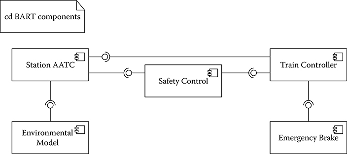
FIGURE 5.16 Component diagram for Bay Area Rapid Transit system.
Figure 5.17 depicts a sequence diagram capturing the common control scenario for the BART system. The figure represents the Issue New Commands diagram referenced earlier in Figure 5.6. This model is annotated with MARTE time constraints to specify the real-time requirements of the BART case study. The behavior specified in the diagram is the following:
Station AATC sends a request to Environmental Model to compute the commands for the train.
Environmental Model computes the commands, taking into account all parameters such as passenger comfort, schedule, etc.
After receiving the commands from Environmental Model, Station AATC sends the commands to Safety Control to ensure the commands computed are safe.
If the commands are safe, Safety Control forwards them to Train Controller.
Train Controller informs Emergency Brake that the commands have been received.
Emergency Brake acknowledges the commands received.
Finally, Train Controller controls the train engine according to the commands received.
In Figure 5.17, we annotated two time instants t0 and t1 using Timed InstantObservations as defined in MARTE, which is indicated by the graphical representations @t0 and @t1. A TimedInstantObservation denotes an instant in time associated with an event occurrence (e.g., send or receive) and observed on a given clock. t0 is the instant when the message Compute Commands is sent by Station AATC, whereas t1 is the time instant when the message Commands Received is received by Emergency Brake.
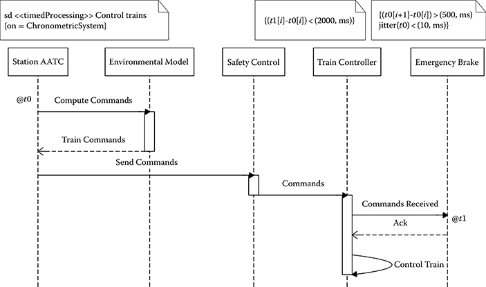
FIGURE 5.17 Sequence diagram for computing and delivering Train Commands.
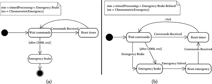
FIGURE 5.18 State-machine diagrams for the Emergency Brake.
Given those two instants, we leverage MARTE to define three time constraints in our system. With the time constraint (t1[i] − t0[i]) < (2000, ms), we limit the duration of each iteration of this scenario to 2 s. The notations t0[i] and t1[i] represent the generic ith instantiation of the scenario (recall that the system operates in cycles). The second constraint, (t0[i + 1] − t0[i]) > (500, ms), imposes that between each instantiation of the scenario, at least half a second passes. Finally, the last constraint, jitter(t0) < (10, ms), limits the jitter of the t0 event, enforcing that between each iteration of the event at t0, there are between 500 and 510 ms.
Figures 5.18a and 5.18b present state-machine diagrams for the Emergency Brake system. These state machines are two different versions of the same perspective, where the one in Figure 5.18b is a refined version that enables restarting the system after an emergency brake. If we consider the three graphs from Figures 5.16, 5.17, and 5.18a together, we have an inconsistent model: the state machine diagram Figure 5.18a does not acknowledge the Commands Received call from Train Controller—contrary to what the sequence diagram from Figure 5.17 demands. Replacing the diagram from Figure 5.18a with Figure 5.18b, we obtain a consistent model.
5.5 Discussion and Open Issues
UML is a well-established language, with advanced tool support and an active community of developers that evolve the standard. The language has been developed with the goal of having a general purpose modeling language. It supports different types of systems, in different domains, and people with different backgrounds and expertise. This flexibility is the main strength of the UML. However, flexibility has a price. Many of the issues reported by researchers in working with the UML originate from the design decision of making it flexible and adaptable to multiple usage scenarios. In particular, problems arise in the field of UML model consistency, system synthesis, and model transformation.
In the following, we discuss to what degree UML meets the requirements for modeling languages identified in Section 5.2.
Consistency. As discussed in Section 5.3.4, the semantics of UML is open for extensions. The UML standard from OMG does not provide a complete formal semantics and leaves many options in the language open for specialization. However, having formal semantics is a key enabler both to supporting model consistency and to leveraging UML in safety-critical systems. In fact, for safety-critical systems, it is often mandated to formally prove various properties. Moreover, in the domain of real-time systems, some level of semantics is required to support analysis tools, such as tools for scheduling. Because of its incomplete semantics, UML cannot be used directly for real-time systems simulation and verification. Profiles such as MARTE aim at adding sufficient semantics to the UML to support analysis tools.
Traceability. UML use case diagrams have been traditionally used to document requirements, but they have a number of limitations including their lack of well-defined semantics. Other diagrams such as sequence diagrams can be used for requirements engineering to model the next level of detail from use cases. However, the relation between the requirements models (see Section 5.3.2.1) and the architectural ones (see Section 5.3.2.2) is typically difficult to trace in the UML. SysML adds requirements modeling as a key engineering activity and it provides traceability to requirements throughout the design flow; in SysML, a requirement can be related to a model element that satisfies or verifies the requirement. However, the requirements notion of SysML is again not a formal one, and thus not immediately amenable to a precise modeling approach in relation to the associated architectural models. Furthermore, MDA—also an OMG standard—supports traceability within the architectural models from PIM to PSM, both specified in UML. In fact, a PSM is obtained from a PIM through a series of transformations, although the platform model is often hard-coded in the transformation. Through its various subprofiles, MARTE provides support for making platform models explicit. Therefore, platform models can be an explicit input to the model transformation for the target platform.
Realizability. UML models have several uses. In the real-time domain, they are often used to verify system properties (even before building the system) and to generate part of the implementation. A problem that can arise is that it is not possible to realize the model, given some implementation constraints. For example, constraints on the CPU could make it impossible to fulfill some timing constraint. Therefore, it is important to always revise the models during the development process to ensure that all assumptions taken in analyzing models are fulfilled by the implementation.
Distribution and integration. A key issue in modeling large embedded systems is that the modeling activity is often distributed across different teams and even different organizations. In cases where the modeling activity is distributed, the UML must support independent modeling of different parts of the system, which will cause conflicts and inconsistences. Therefore, projects with distributed models must establish a model integration process and leverage tools to manage inconsistencies.
Interdisciplinary domains. Through its built-in profile mechanism, UML can be tailored for various domains or different target platforms. Defining a custom domain-specific language ab initio has the advantage that the language can be optimized for the target domain, but complex systems often have various concerns that are modeled separately, and integrating models defined in different languages is not an easy task. The advantage of UML is that it provides an integrated framework, where profiles specialize UML concepts and, therefore, can be used with existing UML tools. Nevertheless, if the interdisciplinary application requires combining more than one UML profile, there are significant issues with overlapping and inconsistent language specification across the two profiles, especially when the two disciplines to be integrated are sufficiently close so that their domain representations in the respective profiles overlap. These issues necessitate careful, domain-specific integration of the profiles, because the UML itself provides no strong interface concept for profiles
Nonfunctional properties. Several UML profiles including SPT, QoS & FT, and MARTE provide extensions to support various nonfunctional properties. MARTE allows specifying properties such as throughputs, bandwidths, delays, and memory usage, and these follow a well-defined textual syntax—MARTE introduces the VSL to formulate algebraic and time expressions. VSL is based on OCL but also provides time-related annotations. Section 5.4.2 provides more details on the specification capabilities of MARTE. Notably, UML models can be annotated with nonfunctional properties, given that annotation is a nonintrusive operation on an existing model to add additional information necessary for analysis. For example, MARTE can be used for requirements engineering to annotate nonfunctional requirements in use cases and the corresponding sequence diagrams.
Resource models. MARTE provides a taxonomy for software and hardware resources, which support specifying computing platforms at different levels of abstractions and with their corresponding nonfunctional properties such as memory usage and power consumption. Support for modeling time, resources, allocation, and other qualitative and quantitative concerns is included in various subprofiles in MARTE. Other work [19] discusses the coverage provided by each subprofile. For example, resource modeling is addressed by the GRM, SRM, HRM, GQAM, SAM, PAM, and RSM subprofiles (see Section 5.4.2).
Timing. The time model in UML is trivial, but MARTE provides significant extensions and supports three models of time: chronometric, logical, and synchronous. MARTE provides fundamental time notions such as time instant, duration, time bases, and clocks, while it supports multiple time bases for distributed systems. MARTE also introduces the key concept of observation, which enables a time constraint to be specified as a predicate on timed observations. Moreover, time concepts are not just annotations but they are defined as part of the system behavior.
Heterogeneous models of computation and communication. Several embedded systems require more than one model of computation to reflect the nature of the application domain, whereas UML supports only event-based models. Therefore, several proposals have been made to extend UML with support for continuous time by using stereotypes to represent continuous variables, time, and derivatives [28]; a programming language for hybrid systems [29]; and a dataflow mechanism (distinguishing between signal ports and data ports) coupled with mathematical equations, called D-UML [30]. The model of computation in MARTE is an asynchronous/event-based approach but alternative models can be defined as extensions to the MARTE specification.
5.6 Summary and Outlook
In this chapter, we have presented UML and some of its profiles specifically tailored for real-time systems. Using specific profiles, UML models can be leveraged for design and analysis during the development of real-time embedded systems. Models are a key asset in complex embedded systems, as they provide reusability across product generations, help in eliciting and specifying requirements, facilitate integration of components developed by different suppliers, support system verification before deployment, and support synthesis and deployment.
UML has evolved over the years to support more modeling techniques and adapt to novel tasks. In its latest incarnation 2.3, UML is a substantial improvement over the original version. As noticed in other works [10,45], UML has maintained many promises but has still some pitfalls that limit its utility.
The main promises it maintained are the support for multiple notations as part of a single language and the support for profiles to modify the language and its semantics. Furthermore, UML is supported by a plethora of tools to create and analyze models.
The main pitfalls attributed to UML are concerned with its complex and bloated metamodel, which makes it difficult to master the language in its details, and the lack of semantics associated to some elements (i.e., aggregation), which creates confusion and different interpretations from different tool manufacturers.
In this chapter, we presented the facilities of UML for dealing with time. UML 2.x can specify time properties by means of Time Duration and Observation (of time passing). The basic time facilities and time constraints are, however, too simple to address requirements of real-time systems. The UML standard itself suggests using a profile (see the UML Superstructure standard document [3] Chapter 13) to enhance the ability to specify time properties. Following this suggestion, MARTE adds a comprehensive ontology of time and a language, VSL, to write time constraints. In addition, SysML provides facilities to support continuous time in addition to discrete events.
More research is required to unlock the full potential of the UML and to make it more applicable to the real-time systems domain. In particular, the UML metamodel should be restructured and streamlined to simplify the definition of semantics variations and the creation of tools. Specifically, the current language specialization facilities (such as profiles) require a profound understanding of most of the complex UML metamodel. Furthermore, the specialization builds upon the full metamodel, adding further elements and relations (as we have shown for MARTE in this chapter). Therefore, the use of a particular profile implies a profound understanding of all of the UML intricacies plus the ones added by the profile. A substantial usability improvement would emanate from an option to eliminate parts of the metamodel that are irrelevant for a given application domain.
The other part of UML that requires substantial improvement is the semantics definition. The existence of alternative semantics for some elements and the absence of semantics for others confuse users of the standard. Profiles are supposed to lock down the semantics of some elements. However, the existence of different interpretations for the meaning of some modeling elements increases the chances of models being misinterpreted by users who are not experts in a particular profile.
Moreover, UML does not provide the necessary support for checking and enforcing model consistency. Modeling involves multiple diagram types (thus, multiple modeling languages) that focus on specific aspects of a system. Therefore, ensuring consistency between models is key for system synthesis and analysis. In Chapter 12, we will focus on the topic of model consistency for UML and cover the issues of consistency checking, assigning semantics to UML diagrams and integrating multiple models into a coherent system model.
Acknowledgments
This work was partially supported by the NSF within projects CCF-0702791 and CNS-0963702 and by funds from the California Institute for Telecommunications and Information Technology (Calit2) at the University of California, San Diego. We are grateful to Barry Demchak and the anonymous reviewers for insightful comments.
References
1. Giese, H., G. Karsai, E. Lee, B. Rumpe, and B. Schätz. 2011. Model-Based Engineering of Embedded Real-Time Systems, Vol. 6100. Berlin/Heidelberg: Springer.
2. Object Management Group. 2010. “Unified Modeling Language (OMG UML), Infrastructure, Version 2.3.” formal/2010-05-03, OMG.
3. Object Management Group. 2010. “Unified Modeling Language (OMG UML), Superstructure, Version 2.3.” formal/2010-05-05, OMG.
4. Sprinkle, J., B. Rumpe, H. Vangheluwe, and G. Karsai. 2011. “Metamodelling: State of the Art and Research Challenges.” In Model-Based Engineering of Embedded Real-Time Systems, edited by H. Giese, G. Karsai, E. Lee, B. Rumpe, and B. Schätz, Lecture Notes in Computer Science, Vol. 6100, pp. 57–76. Berlin/Heidelberg: Springer.
5. MathWorks. 8 April 2011. MATLAB. 7.12. http://www.mathworks.com/products/matlab/.
6. MathWorks. 8 April 2011. Simulink. 7.7. http://www.mathworks.com/products/simulink/.
7. ETAS. April 2011. ASCET. 6.1.2. http://www.etas.com/sen/products/ascet_software_products.php.
8. Object Management Group. 2003. “Model Driven Architecture (MDA) v1.0.1.” omg/ 03-06-01, OMG.
9. Nicolescu, G., and P. Mosterman. 2009. Model-Based Design for Embedded Systems, pp. 766. Boca Raton, FL: CRC Press.
10. France, R., and B. Rumpe. 2007. “Model-Driven Development of Complex Software: A. Research Roadmap.” In Proceeding of Future of Software Engineering (FOSE’07), L. Briand and A. Wolf (Eds.), pp. 37–54. Minneapolis, MN, USA, Los Alamitos, CA: IEEE Computer Society.
11. Sztipanovits, J., and G. Karsai. April 1997. “Model-Integrated Computing.” Computer 30 (4): 110–11. Los Alamitos, CA: IEEE Computer Society.
12. Balasubramanian, K., A. Gokhale, G. Karsai, J. Sztipanovits, and S. Neema. 2006. “Developing Applications Using Model-Driven Design Environments.” Computer 39 (2): 33–40 Los Alamitos, CA: IEEE Computer Society.
13. Fowler, M. 2004. UML Distilled Third Edition: A Brief Guide to the Standard Object Modeling Language. Boston, MA: Addison-Wesley.
14. Pretschner, A., M. Broy, I. H. Krüger, and T. Stauner. May. 2007. “Software Engineering for Automotive Systems: A Roadmap.” In Proceeding of Future of Software Engineering (FOSE’07), L. Briand and A. Wolf (Eds.), pp. 55–71. Minneapolis, MN, USA, Los Alamitos, CA: IEEE Computer Society.
15. Department of Defense. 2010. “The Department of Defense Architecture Framework (DoDAF) Version 2.02.” DoD.
16. Boehm, B. W. 1988. “A Spiral Model of Software Development and Enhancement.” Computer 21 (5): 61–72 Los Alamitos, CA: IEEE Computer Society.
17. Winter, V., F. Kordon, and M. Lemoine. 2004. “The BART Case Study.” In Formal Methods for Embedded Distributed Systems, edited by F. Kordon, and M. Lemoine, pp. 3–22. New York: Springer.
18. Object Management Group. 2009. “UML Profile for MARTE: Modeling and Analysis of Real-Time Embedded Systems” Version 1.0, formal/2009-11-02, OMG.
19. Gérard, S., H. Espinoza, F. Terrier, and B. Selic. 2011. “Modeling Languages for Real-Time and Embedded Systems: Requirements and Standards-Based Solutions.” In Model-Based Engineering of Embedded Real-Time Systems, edited by H. Giese, G. Karsai, E. Lee, B. Rumpe, and B. Schätz, Lecture Notes in Computer Science, Vol. 6100, pp. 129–54. Berlin/Heidelberg: Springer.
20. Horowitz, B. 2003. “Giotto: A Time-Triggered Language for Embedded Programming.” Doctoral Dissertation, University of California, Berkeley.
21. Henzinger, T. A., C. M. Kirsch, M. A. A. Sanvido, and W. Pree. February 2003. “From Control Models to Real-Time Code Using Giotto.” 23 (1): 50–64. New York, NY: IEEE Control Systems Magazine,
22. Henzinger, T. A., B. Horowitz, and C. M. Kirsch. 2001. “Embedded Control Systems Development with Giotto.” In Proceedings of the ACM SIGPLAN workshop on Languages, Compilers and Tools for Embedded Systems (LCTES’01), pp. 64–72, New York, NY, USA: ACM.
23. Templ, J. 2008. TDL: Timing Definition Language 1.5 Specification, preeTEC GmbH.
24. Farcas, E., C. Farcas, W. Pree, and J. Templ. 2005. “Transparent Distribution of Real-time Components Based on Logical Execution Time.” In Proceedings of ACM SIGPLAN/SIGBED Conference on Languages, Compilers, and Tools for Embedded Systems (LCTES), pp. 31–9. New York: ACM Press.
25. Object Management Group. 2006. “Meta Object Facility (MOF), Version 2.0.” formal/2006-01-01, OMG.
26. Douglass, B. 2004. Real-Time UML: Advances in the UML for Real-Time Systems. Boston: Addison-Wesley.
27. Douglass, B. 2003. Real-Time Design Patterns: Robust Scalable Architecture for Real-Time Systems. Boston: Addison-Wesley.
28. Douglass, B. P. 1999. Doing Hard Time: Developing Real-Time Systems with UML, Objects, Frameworks, and Patterns, pp. 800, Boston: Addison-Wesley.
29. Warmer, J., and A. Kleppe. 1998. The Object Constraint Language: Precise Modeling with UML, pp. 144, Boston: Addison-Wesley.
30. ITU. 1996. “Message Sequence Charts (MSC).” ITU-TS Recommendation Z.120.
31. Krüger, I. H. 2000. “Distributed System Design with Message Sequence Charts.” Doctoral Dissertation, Technical University of Munich, Germany.
32. Broy, M., M. Crane, J. Dingel, A. Hartman, B. Rumpe, and B. Selic. 2007. “2nd UML 2 Semantics Symposium: Formal Semantics for UML.” In Models in Software Engineering, edited by T. Kühne, Lecture Notes in Computer Science, Vol. 4364, pp. 318–23. Berlin/Heidelberg: Springer.
33. Selic, B. 2004. “On the Semantic Foundations of Standard UML 2.0.” In Formal Methods for the Design of Real-Time Systems, edited by M. Bernardo, and F. Corradini, Lecture Notes in Computer Science, Vol. 3185, pp. 75–6. Berlin/Heidelberg: Springer.
34. Chen, R., M. Sgroi, L. Lavagno, G. Martin, A. Sangiovanni-Vincentelli, and J. Rabaey. 2003. “UML and Platform-Based Design.” In UML for Real: Design of Embedded Real-time Systems, pp. 107–26. Netherlands: Kluwer Academic Publishers.
35. Selic, B., and J. Rumbaugh. 1998. Using UML for Modeling Complex Real-Time Systems. Objectime Limited.
36. Selic, B. 1998. “Using UML for modeling complex real-time systems.” In Proceedings of the ACM SIGPLAN Workshop on Languages, Compilers, and Tools for Embedded Systems, pp. 250–60. London, UK: Springer-Verlag.
37. Selic, B., G. Gullekson, J. McGee, and I. Engelberg. 1992. “ROOM: An Object-Oriented Methodology for Developing Real-Time Systems.” In Proceedings of 5th International Workshop on Computer-Aided Software Engineering, pp. 230–40. IEEE Computer Society.
38. Krüger, I. H., W. Prenninger, R. Sandner, and M. Broy. 2002. “From Scenarios to Hierarchical Broadcasting Software Architectures using UML-RT.” International Journal of Software Engineering and Knowledge Engineering 12 (2): 155–74 World Scientific Publishing.
39. Krüger, I., W. Prenninger, R. Sandner, and M. Broy. 2004. “Development of Hierarchical Broadcasting Software Architectures using UML 2.0.” In Integration of Software Specification Techniques for Applications in Engineering. Priority Program SoftSpez of the German Research Foundation (DFG). Final Report, edited by H. Ehrig, W. Damm, J. Desel, et al., Lecture Notes in Computer Science, Vol. 3147, pp. 29–47. Berlin/ Heidelberg: Springer.
40. Object Management Group. 2005. “UML Profile for Schedulability, Performance, and Time, Version 1.1.” formal/05-01-02, OMG.
41. Object Management Group. 2008. “UML Profile for Modeling Quality of Service and Fault Tolerance Characteristics and Mechanism, Version 1.1.” formal/2008-04-05, OMG.
42. Object Management Group. 2010. “Systems Modeling Language Version 1.2.” formal/2010-06-01, OMG.
43. Espinoza, H., D. Cancila, B. Selic, and S. Gérard. 2009. “Challenges in Combining SysML and MARTE for Model-Based Design of Embedded Systems.” In Model Driven Architecture: Foundations and Applications, edited by R. Paige, A. Hartman, and A. Rensink, Lecture Notes in Computer Science, Vol. 5562, pp. 98–113. Berlin/ Heidelberg: Springer.
44. Feiler, P. H. 2009. The SAE Architecture Analysis & Design Language (AADL), SAE International Document AS-5506A ed.
45. France, R. B., S. Ghosh, T. Dinh-Trong, and A. Solberg. 2006. “Model-Driven Development Using UML 2.0: Promises and Pitfalls.” Computer 39 (2): 59–66 Los Alamitos, CA: IEEE Computer Society.