18 Simulation for Operator Training in Production Machinery
Gerhard Rath
CONTENTS
18.1.1 Ultra Flexible Reversing Mill
18.1.2 Simulation for Operator Training
18.1.5 Game-Based Learning, Game Programming, and Simulation
18.2 Simulation of Plant and Machinery
18.2.1 Languages for Simulation
18.2.2 Recent Developments and Trends
18.3 Simulator for Rolling Mill Operator Training
18.3.1 Requirement Analysis of the Training Simulator
18.3.2 System Design of the Training Simulator
18.3.3 Reduction of Complexity
18.3.3.2 Reduction of Possible Machine States
18.3.3.3 Reduction of States by the Control Program
18.3.4 Simulation Tool Selection and Program Coding
This chapter describes the development of and the experience with a training simulator for a steel rolling mill. The goal of the training is how to replace the rolls, which is normally controlled by the electronic system, but has to be done in certain exceptional situations by the operators or the maintenance personnel without automatic sequence control. The actual machine is not available for training, since the production is fully automated and is running around the clock. This operator training simulator (OTS) replaces the functionality of the machine in a loop with a replica of the electronic control system (hardware-in-the-loop, HIL). Simulation is applied to train the operators and the maintenance staff. To keep the staff well trained without the necessity to interrupt the production routine of the machine was the motivation to develop the simulator.
The introduction describes the basic considerations that were necessary for a successful development project. In the second section, the status of simulation in industrial production plants is discussed, where it is noted that simulation is of fast growing significance in this field. The third section presents details of the simulator design and some interesting particularities that were found during the project. Finally, the experiences acquired over several months are given.
18.1 Introduction
After a short description of the actual simulation problem, a brief overview of past and present trends in simulation-based operator training is given. The third subsection shows some important aspects of modeling from the view of software engineering. For simulation of fast physical systems such as machines, considerations of real-time aspects are important. Finally, a look at the impact of modern computer games to the development of simulation software is useful before starting the modeling work.
18.1.1 Ultra Flexible Reversing Mill
Voestalpine Schienen GmbH is a leading manufacturer of rails and is exploiting a new ultra flexible reversing mill consisting of three identical mill stands [1]. The automation system of the mill provides all necessary control for production, which includes the basic sequential and closed-loop control of the movements of the mechanical equipment and the technological process control such as minimum tension control.
In normal operation, the complex roll exchange is a process of maintenance and runs fully automated under supervision of the control system. With the help of hydraulic and electric systems, three systems of horizontal and vertical rolls are exchanged. The process goes through about one hundred steps and requires hundreds of actuators and an even larger amount of sensors. Sometimes a failure in the system occurs, and the automatic cylce stops. Then, after a repair, the steps must be carried out without automated sequencing. The danger of making a mistake and damaging some components is high. Such mistakes increase the downtime of the machine significantly. More and regular sessions with a systematic training program are necessary for faster performance. A long period of continuous production, which is of course a desirable advantage, turns out to be a problem for the maintenance personnel, since they have fewer opportunities to train and hone their skills. This was the reason for the development of the training simulator.
18.1.2 Simulation for Operator Training
The need for training simulation emerged when human mistakes during the operation of technical devices started causing harm to people. Beginning with mechanical simulators in the first decades of aviation, the first computer simulations appeared in the 1960s. Flight simulators for the training of operators of airplanes [2] and spacecraft were indispensable. In addition to modeling and simulation, pedagogical frameworks based on training modules were developed to lead the trainee step-by-step through the basics of operation.
The high cost of such equipment is why such simulators were introduced very late to industrial equipment. Nuclear power plants with their high risks were the first to see computer simulation employed [3]. The chemical industry and fossil power plants followed. Recent progress in computer technology, hardware, and software have reduced the cost and enabled the use of simulation also in industries with lower risk and impact, such as heavy machinery [4].
While conventional training requires access to resources dedicated to production (machine, plant, people), simulation on the computer reduces the danger caused by mistakes of the trainees, and also the cost of potential damage. Beside these points, making the original system available for training reduces the production capacity and is a more recent argument in favor of OTS. For accurate simulation, models for the physical or chemical processes are controlled by a replica of the deployed control system. Having the simulation in a loop with a piece of original hardware is referred to as HIL [5,6].
Other fields of training simulation emerge for highly complex systems. For example, the optimization of the market of electrical power supply [7] necessitates optimal operation of the power grid [8]. For medical appliances, training simulation is also well established [9]. A demographic problem, the retirement of aged experts that results in a lack of training facilities for the apprentices, is proposed to be solved with training in simulation [10].
Embedded simulation is a recent development in military appliances to bring training closer to high fidelity environments. When not in action, weapons can temporarily switch to a simulation mode for training. This allows training not only in training centers and classrooms but also in the actual place of operation. The environment is more realistic and training can occur more often during standby times. Civil equivalents of this technique are conceivable.
18.1.3 Modeling
Before a simulation of a system can be carried out, a model must be established. Different definitions for a model exist in several standards or books; a useful one can be found in Lieberman [11]:
A model can be defined as the simplification of a complex system for the purpose of communicating specific details.
Definition of a model
Lieberman
The emphasis should be on the word “communication,” telling us that the purpose of a successful modeling process is not to create a model, but to inform a hopefully well-defined group of people about some selected details of the system under study that is modeled. A model should not be built until the modeler understands the intended audience. The same author describes an important property of a model:
A model operates much like a lens: It focuses attention on items while obscuring or omitting everything else!
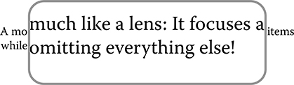
FIGURE 18.1 Focusing effect of a model. (Adopted from Lieberman, B. A. “The Art of Modeling, Part I: Constructing an Analytical Framework,” 2003, accessed July 3, 2010, http://download.boulder.ibm.com/ibmdl/pub/software/dw/rationaledge/aug03/fmodelingbl.pdf.)
Figure 18.1 explains this property. We and our customer have to accept that a model cannot represent all details of the real system. Trying this, we would fail.
If a system should be modeled for different purposes, different modeling procedures, methods, and tools are applied [12]. In general, separate models for the same plant may be required for, for example, presentation of a machine to salespeople, investigating technical details of the plant behavior, optimizing production and logistic properties, and training of operators.
After the requirement analysis for the modeling development is completed, the design may follow one of the strategies:
Top-down
Bottom-up
Inside-out
Hardest first
These are the same strategies we know from the software development process. The application of the first three strategies is described in Lieberman [13]. For the steel rolling mill project described in this chapter, the “hardest first” approach had to be applied, since the behavior of some critical parts of the system were not known exactly and had to be explored first.
Before starting the modeling process, a classification is helpful to select the best-suited language or tool for the actual purpose. A useful classification may be according to Figure 18.2. For continuous models, time is a primary simulation variable. This is the way we describe dynamic systems starting from ordinary differential equations (ODE), applying Laplace transform and transfer functions [14]. Time-based models running on a computer are inherently of a discrete nature. This means that modeling of dynamic systems requires the z-transform to obtain digital transfer functions. Modern modeling languages such as Simulink® [15] are capable of masking this difference and even allow running discrete-time and continuous-time models concurrently within one system. This simplifies the modeling task and saves us from working with z-transform or similar techniques. Event-based models are used when the system primarily reacts to events happening at certain time points, and the state of the system does not change over time between two subsequent events. Finite state machines (FSM) are one example of a basic method to implement such a model. Again, it is state of the art to have continuous-time, discrete-time, and event-driven models combined in a single computer model. Finally, process-based models were developed to map workflow processes of practical value into a simulation model, for example, Business Process Modeling Notation [16].
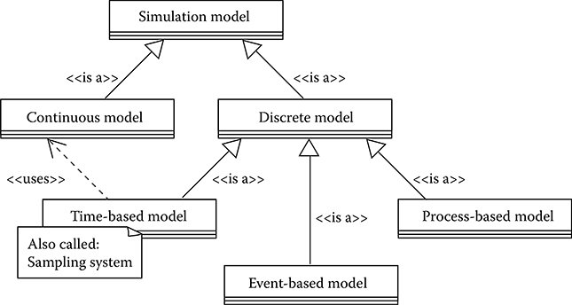
FIGURE 18.2 Classification of mathematical models for simulation.
18.1.4 Real-Time Simulation
A simulator for operator training requires a real-time response. This means the time behavior of the simulation must match with the physical system. The definition “real time” demands that the computations that are necessary in a given time interval can be completed in this specified time interval [17]. Not only the calculation of the models, but also data communication must abide by this restriction [18]. Usually, the real-time property is obtained by the utilization of a dedicated operating system. In computers for human–machine interface (HMI), often a standard operating system with some real-time extension is used. Even if the “hard” real-time property cannot be guaranteed, such systems are proven to work properly as simulators. The chosen environment for the actual steel rolling mill project, Winmod®, is one of this type [19].
18.1.5 Game-Based Learning, Game Programming, and Simulation
Modern computer games are an important pacemaker for developments in the computer industry. So it is worth it to take a look at game programming when investigating the facilities of modern simulation.
Game-based learning (GBL) is an integrated part of eLearning [20]. Even if no GBL is intended, the target audience, the trainees on the simulator, may have grown up with computer games and acquired a different cognitive character (“gamer generation” [21]). Games are applied in learning environments to increase the motivation. Fantasy, rules/goals, stimulus, challenge, mystery, control, and feedback are the characteristics of a game that augment the learning effect [22].
Exploring the possibilities of new media causes enthusiasm, but one must be cautious about the eLearning hype. A game is only a game in a narrower sense, if there is no purpose behind it [23], and people who often play games are more critical about serious games [24].
For the designer of a training simulator, the following aspects may be important.
Playing the Simulation Game. A simulation itself is to an extent a game that models parts of the actual world [25]. The topic of simulation for training is given by the actual task, but for presentation, visualization, etc., we can gain inspiration from eLearning and GBL on how to design an attractive environment for the simulation.
Trainer or GBL Environment. Most OTS for industrial production systems require a trainer to guide through a session. This trainer usually observes and rates the session. If the reaction to a fault needs to be trained, the trainer provokes a failure at a certain instant. Substituting this trainer with software would be a step towards GBL.
Game Programming. For the developer of simulation software, game programming is a rich source of methods and techniques. All required design patterns on how to create successfully virtual worlds for a trainee are developed and published. For example, work has been done on how to design the architecture for simulation in real-time and visualize it in 3D [26]. To model the dynamic behavior of game characters or machines, work that employs FSM, parallel or nondeterministic automata can be found [27]. Scripting techniques that simplify rich but complex programming languages as those employed in design patterns are ideally suited for industrial programmers.
18.2 Simulation of Plant and Machinery
Because of high costs, the application of simulation has been limited to industry and organizations with a high level of risk. Today simulation is also becoming prevalent in the production industry. Shorter product cycles, flexible production, risk reduction, and more competition give a good return on investment to simulation techniques.
This highly dynamic process is still ongoing, so the vocabulary of simulation is not standardized yet for the production industry. In contrast, for flight simulators, the requirements were defined much earlier [28]. The following classification and keywords are based on some definitions of the German chemical industry [29], on the specifications of a supplier for simulation systems [19], and on personal discussions [30].
Control System Tester. Such simulators are used to test the function of the control systems; this is a verification of the control software.
Process Trainer. Process trainer simulations are not used to verify the function of the automation system, but focus on the simulation of process dynamics. The trainees learn to understand a complex, physical, or chemical process.
Virtual Startup. The control system can be tested and commissioned while connected to virtual machinery. This is designated a virtual startup. Since the control system is the same that will later be working with the physical plant, it should be mentioned that, from the viewpoint of the control system, it is a real startup [30]!
Factory Acceptance Test (FAT). A simulation model of a complex production plant and its control system can be subjected to a FAT. Logistic chains, dynamic and logical properties, capacities etc. can be verified with the participation of the customer before delivery and assembly of the actual system. This is progress in the sense of “Simultaneous Engineering” [31]. Mistakes in the requirement specifications, planning mistakes, and critical states of the machinery are detected without risk in an early phase and save time during the startup of the plant.
Functional Validation. With the customer involved, the software is checked against the requirements. It is not the goal here to find programming errors, which should be already removed by verification, but misunderstandings between the supplier and the customer [30]. Without simulation, usually this validation is carried out during commissioning of the plant. With the help of simulation, it is possible to correct such errors much earlier.
Design and Planning. In an early project phase, simulation allows us to find mistakes in planning caused by incompatibilities between different engineering departments. For example, the variables used for controller programming may not correspond to the inputs and outputs as defined by the electric engineers. Without simulation, such errors can be detected only very late during the assembly or the startup phase.
Instruction and Training. OTS work with a replica of the automation system. Training and instruction can proceed without the physical plant. Usually this is used to shorten the startup of the actual plant. OTS are working in the loop with the actual process control system (HIL). It is desired to include defined scenarios of plant failures (“what if” scenarios [29]).
Maintenance and Optimization. After the startup of the real plant, the simulation helps optimize parameters and find causes of problems. The simulation can run parallel to the physical plant and avoids the necessity of interaction with and perhaps disturbance of production.
Presentation. A virtual presentation of the plant can support the salespeople and brings advantages over the competitors. Of course, the quality of the presentation is more important than the technical accuracy.
It is desired that one system should provide all these features, which is the goal of developers of modern simulators [19].
In production machinery, it is not possible to obtain a fully detailed physical fidelity of simulation since the reaction times are much shorter than in chemical processes. This is shown in an example in Section 18.3.3 and is one of the reasons why a certain component is modeled for different purposes with different tools [12].
18.2.1 Languages for Simulation
The problem to choose the most suitable language for a simulation of an industrial equipment is closely related to the selection of languages for the electronic control of the system; consequently, at first a look to these languages is required.
The control of machinery and plants in the production industry has been done with electronic systems since the 1980s. Before this, relay control was the state of the art. Free programmable systems (PLC, programmable logic control) emerged in the 1990s [32,33]. Those systems provided a restricted command set for programming, on the one hand to minimize the danger of mistakes and on the other hand to guarantee that persons different from the programmer could read, understand, and modify the code. From this point of view, programmers for industrial systems must be specialists in the specific process, more so than in ultimate software techniques. Standardization of languages led to Continuous Function Chart and the languages defined in the IEC 1131 standard becoming the most important representatives [34].
The languages are based on graphical concepts such as electric circuit diagrams and FSM and on textual concepts such as assembler, Basic, and Pascal. Object orientation is implemented to a limited extent. New objects may be created “by composition,” which means putting existing objects together to create new ones. Multiple inheritance and dynamic binding are not used.
The basic idea for all these restrictions and simplifications is to construct control programs that can be grasped by other process experts independent from their writers.
Now the same also applies for simulation programs. Machine and process experts should be enabled to develop models and their behavior, and the visualization and real-time monitoring of the simulated process. For example, MathWorks recently published an extenstion for Simulink to create IEC-1131-compatible programs [35].
The choice of the language for simulation is a trade-off between the versatility of a modern computer language and the maintainability of the software by people who are more process experts than software experts. For the actual project of the rolling mill simulator, the selected system [19] provides a graphical programming suite similar to Function Block Diagram, which is one of the languages defined in the IEC 1131 standard.
18.2.2 Recent Developments and Trends
All components of control systems for production machinery must provide interfaces to supplemental products of other manufacturers, for example, standard fieldbus systems or OPC communication (OLE for process control). Products for simulation must follow this trend since for different purposes different simulation environments are established.
Suppliers generate many documents to design a system. The ideal case is to generate a simulation completely automated from these documents with a minimum of further programming effort.
In regard to operator training, a simulation must provide possibilities to train exceptional situations. For example, the nuclear power industry has well-defined training scenarios for exceptions. Many industrial simulation systems work with a trainer who provokes an error during the session or defines the errors immediately before the start. Script-based or FSM techniques should make it easier to define training scenarios.
18.3 Simulator for Rolling Mill Operator Training
This section describes development work for the actual simulator in a time-ordered manner. First, the requirements are specified, then the design of the software components follows. Taking into consideration how to reduce the enormous complexity to a reasonable extent is important before selecting a tool and doing the coding work.
18.3.1 Requirement Analysis of the Training Simulator
From the basic considerations described in Section 18.2, some conclusions are drawn: The language for developing training simulators should be one of the typical industrial languages so that machine experts can understand and change the program code of the simulator. C++ or other object-oriented languages, which offer more freedom to the programmer, but may result in unreadable code, are not favored. A training session should not have a game character and no success indicators of a training session should be recorded, since this is demanded by the trade union. The behavior of some critical machine parts are typically not known in sufficient detail so as to initiate their modeling without further preliminary analysis. Consequently, the hardest-first approach to design is to be applied.
The application of a use-case analysis turned out to be a successful part in the phase of requirement specifications. A simplified use-case diagram is shown in Figure 18.3. The machine operator commands the automated roll exchange as well as the manual exchange. In case of problems, a second actor, the maintenance expert, works on the “manual roll exchange.” For training purposes, the simulator should substitute the physical machine for a use case “manual roll exchange.”
During the automated production, the roll exchange also runs autonomously, and the operator supervises the procedure. In the case of a failure in the system, the roll exchange must be done by the operator, thought not manually, on a low level of automation. Several hundred drives must be coordinated in about one hundred steps. After a repair, the machine must be brought into a condition where the automatic sequence may continue. Figure 18.4 shows the configuration of the actual system and the data flows among the components. The operator works with his HMI and a replica of the control system. Several hundred inputs and outputs must be communicated in real time between the control system and the simulator. To avoid the cost of copper wires, serial communication over an industrial fieldbus was the choice.
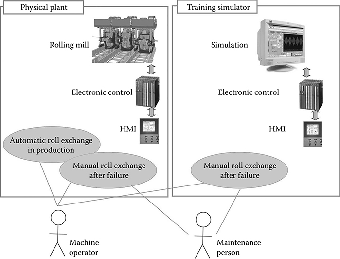
FIGURE 18.3 Use cases of the roll exchange task.
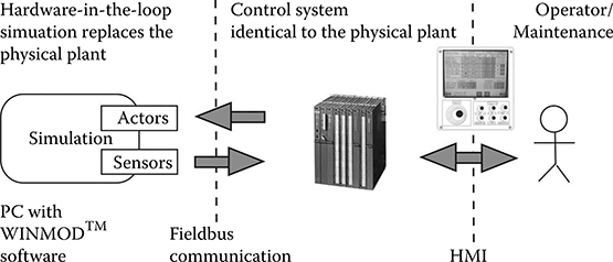
FIGURE 18.4 Hardware configuration of the training simulator.
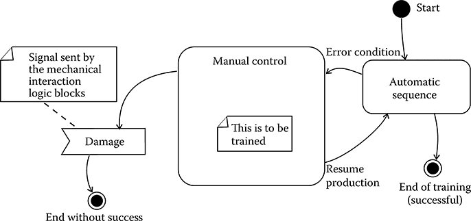
FIGURE 18.5 State diagram of the training session.
18.3.2 System Design of the Training Simulator
As a first design step, based on the requirement analysis and on the introductory considerations, the course of the training session was defined. It can be documented as a state diagram (see Figure 18.5), according to UML notation [36]. Two exits are designed. One is the successful end, when the machine can resume its normal production again. When the trainee causes damage to the system after a mistake, the session is terminated (“game-over” situation).
An important aspect can be found in Figure 18.5: the automatic sequence (which is not a topic for the training) is a milestone for testing the system. All components of the physical simulation are actuated by the control system and the system is running in a continuous mode.
The next design step is to find a structure for the simulation software. The simulator should replace the physical machine and provide its behavior to the replica of the electronic control system (see Figure 18.4). The artifacts of the simulation software are shown in Figure 18.6. Apart from the software component simulating the machine, there exists a visualization part. This is not for the trainee, who works with the HMI of the control system, but is required for administration and adjustments of the simulator. Since the operator of the physical machine cannot observe any process and must rely entirely on her/his operating panel, a three-dimensional visualization was not a requirement of the simulation system.
The exception generator is the component of the software in Figure 18.6 for defining and varying the training scenario. It means that the automatic cycle (see Figure 18.5) breaks and the actual training can start.
Another component of the system in Figure 18.6 is the input/output system. Via communication over a fieldbus, this part has to provide the state of about one thousand data points in real time.
The main component of the training simulator is the actual modeling software. A machine or plant consists of an incredible amount of things moving around, delivering signals or interacting with some other parts. To classify this, the machine was considered to consist of components called subassemblies in Figure 18.6. A subassembly is a constructive mechanical part of the machine. It can be a single lever, a carriage for the rolls, or a complex handling system such as a robot. Artifacts called sensors are mounted on these subassemblies to provide information about positions, pressures, etc., while physics and kinematics of these assemblies are to be modeled. One assembly can carry drive units, which are hydraulic or pneumatic cylinders and motors, or electrical drives. Their task is to convert the output signals of the controller into a mechanical force and to apply this to the mechanic subassembly. The motion as a reaction can be found by solving the ODE. Since unrestricted motion is not possible for all components, additionally collisions must be detected. Such interactions can occur among subassemblies or among drives (in a few cases). An interaction can cause damage, which then is a severe mistake of the trainee. Interactions without damage are usually blocking situations, since the machine consists of rigid bodies. Those situations may be resolved by a reversal motion of the drives and are not an illegal condition of the system.
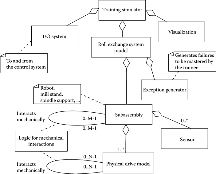
FIGURE 18.6 Objects of the training simulator.
The states of a drive during its simulation lifecycle are shown in Figure 18.7. A normal, successful training end does not terminate the simulation, since the design of the deployed production plant also is made for perpetual operation.
Two points have important implications regarding the design personnel, which are documented in the data-flow diagram in Figure 18.8. The simulator should model the behavior of the machine and its components; consequently, the designers are experts in the mechanical system. The input and output data of the simulation match exactly the sensors and actuators of the deployed system. But this exact mapping concept must be violated. Supplemental data flows must be added (see Figure 18.8):
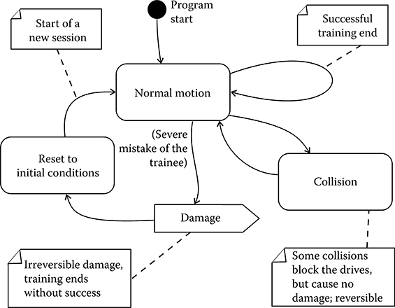
FIGURE 18.7 States that a drive runs through during simulation.
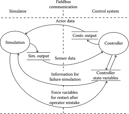
FIGURE 18.8 Data flow between simulator and controller.
The injection of a system fault that the trainee should master is not done by a trainer but automatically in a random manner. This makes it necessary to read the status data out of the control system to determine the instant when a component should fail.
If the trainee causes damage, the entire system must be restarted. It would be too time-consuming to restart the simulator and the control system again. Unfortunately, the machine components cannot fast rewind to their initial positions and states, since the control system does not accept this and would trigger an alarm condition. The solution is to overrule such error conditions by writing internal state variables of the controller.
Both tasks require knowledge of the controller internals. Consequently, it does not suffice to have experts for the physics modeling only, but also control experts who are familiar with the actual controller must be on the team throughout the project.
Furthermore, any intervention in the control system bears the danger that its behavior is changed for the subsequent training session. A mismatch with the physical system would be the consequence.
Now the basic design of the simulator is done. Before a decision for a certain software tool can be made, the complexity of the system should be investigated. Computing time limits the model number of mechanical components and the large number of possible interactions can increase the coding work excessively.
18.3.3 Reduction of Complexity
The most important issue throughout the development process of a simulator is to reduce the complexity to a reasonable extent.
18.3.3.1 Hardware Expense
The simulator replaces the machine or plant and communicates with the clone of the control system. An obvious technique is to connect both systems with wires, as in the physical plant. The communication channel in Figure 18.4 would consist of wires for every input and output. Looking at the cost, this is only affordable for small systems. Consequently, the usual way to establish this communication is to use a fieldbus system, which enables the transfer of thousands of data points with one single cable.
As a further reasonable reduction step, some use a simulation inside the controller running in parallel. Since the exchange of data is done via variables, no additional hardware is required. This minimal configuration is applied for two purposes:
To test some critical parts of the control software
To replace and simulate parts of the physical plant during service operations to establish a normal production cycle
Perhaps this can be called embedded simulation, on-board simulation, or distributed simulation. It should be mentioned that for safety-related systems, this configuration is not acceptable for FAT.
18.3.3.2 Reduction Of Possible Machine States
The components of a typical production machine have interactions that are to be programmed for simulation. The amount of these artifacts should be estimated on the example of the actual project. In the actual project, we call these machine components subassemblies and drives (see Figure 18.6). If each unit can interact with every other, the maximum possible number is a combination by two:
with
N Number of drive units
M Number of mechanical subassemblies
L Number of possble interactions
With the example of N = 40 and M = 8 for one part of the actual rolling mill model, the maximum number of possible interactions will be L = 808. It would not be affordable to program all these interactions. Fortunately, this is only the worst case. The nature of heavy machinery yields a reduction of the number of possible interactions. Manipulators usually are designed to form a linear chain, where each drive can have an interaction with another at the end of its path. For example, a piece of load is handed over to the next at the end position of the first manipulator. Consequently, the amount of interactions is reduced to
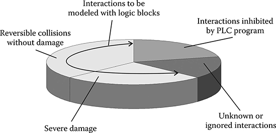
FIGURE 18.9 Interactions of machine parts (collisions).
For the actual example, the number of interactions is reduced to L = 46, which is now realizable.
Additionally, many drives are clamping or locking devices. They have interactions that are possible only at one end of their stroke, which is a further reduction.
18.3.3.3 Reduction Of States by the Control Program
The number of states that must be programmed for the simulation of the machine can be reduced further when we look at Figure 18.9.
Any control logic has programmed manifold interlocks that protect the plant from dangerous conditions and from the most probable operator mistakes. It is possible to exclude these situations to reduce the coding effort, since the PLC will not allow motions leading to them. This saves a lot of development time and also avoids overloading the computing capacity of the simulator. This technique will not be allowed if the purpose of the simulation is to test or commission the control software. But for operator training, this advantage can be taken.
Some collisions are reversible. They block the motion but do not lead to damage. The simulation must provide the opportunity for the operator to take back the move and to continue the training. It is remarkable that the programming of these collisions only requires influencing the motions of parts, but not changing the state of the system. No state logic is necessary to model this kind of interaction.
The number of collisions causing severe damage that must be simulated is now much lower than expected. They must be modeled with state logic that determines the course of the training session.
Furthermore, there always exist interactions with extremely improbable occurence. Provided that the system is not safety critical, we can trust the trainees not to act like monkeys on a typewriter [37] and do not model these situations.
Finally, in every automated system there are unknown states that may cause unexpected incidents even years after commission. But it is not the purpose of an OTS to find such failures.
18.3.3.4 Depth Of Simulation
Dynamic systems in nature are preferably modeled with systems of ODEs, which can be solved numerically with solvers. Applying, for example, Newton’s law yields a model for every mass in a mechanical system. If further we had ideal springs and viscous friction for the interaction among the masses, the resulting model would be a linear time invariant system, which is preferred for the analysis of dynamic systems [14]. This raises the hope to find a model for every thing in the mechanical system, since it consists of discrete, nearly ideal rigid bodies, but this expectation is misleading. Nonlinear springs, Coulomb friction, thermodynamical gas process, and complex kinematics lead to nonlinear equations of motion. Modern simulation environments can cover these effects, but at the expense of increased computing time. Another setback is the occurrence of time responses spread over several powers of ten, which leads to so-called stiff systems in a numerical sense. They are solvable with dedicated numerical solvers that require a higher sampling rate of data and even can cause instabilities in the result [38]. Hydraulic drives are an archetype of a stiff system [39]. Figure 18.10a shows an example from the actual project that is documented in this chapter. A mechanical load model on the right side of Figure 18.10a calculates speed and position from the force input with the help of Newton’s equation of motion. Force is coming from the cylinder model, accepting incoming oil flows to its chambers. The oil pressures are fed back to the proportional valve that determines the oil flow. Tubes are represented by a first-order capacity. To prevent negative cylinder pressures, a counterbalance valve throttles the outgoing oil stream. Finally, a load-sensing pump reduces the supply pressure to avoid loss of power, when high pressure is not required. On a standard PC, this system is not computable in real time. The computation of the load position in the system of Figure 18.10a motion needs ten times more than the counterpart in reality. Since simulation for operator training necessitates the real-time property, we cannot handle even one such drive. Thinking of the modeling discipline given in Section 18.1.3, the system must be simplified by omitting every detail not necessarily required, which is difficult, cumbersome, and time consuming yet critical work during the requirement analysis. For many drives in the actual project, a minimal version of a simple integrator with upper and lower limits as shown in Figure 18.10b was sufficient.
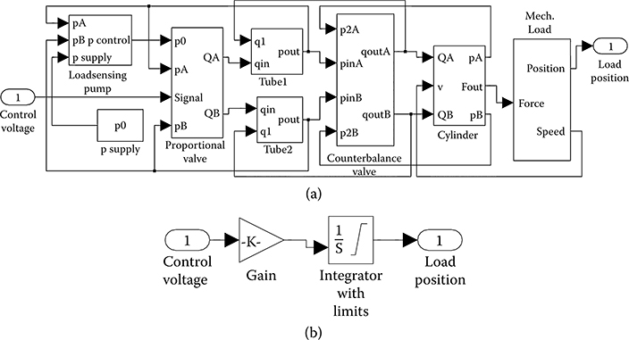
FIGURE 18.10 Models of hydraulic cylinder drives. (a) Extended functionality, including load sensing pump, proportional valve, tube dynamics, counterbalance valves, cylinder, load; (b) ultimate simplification of a drive.
Doing this reduction allowed hundreds of models to run on the computer in real time together with other tasks such as communication and visualization. In conclusion, a thorough simplification during the requirement analysis is recommended to obtain a well-performing simulator.
18.3.4 Simulation Tool Selection and Program Coding
The requirement analysis in the previous sections was a prerequisite for definitively choosing a simulation tool. The training sequence was defined, the model components were classified, and the basic behavior of moving machine parts was identified. All steps were carried out with the aim to minimize the development expense.
Most simulation problems in automation are designed as linear processes. For example, a flight landing simulation requires the operator to follow an exact sequence. Any deviation from the sequence causes the disruption of the training. Or, a chemical process has definite sequence steps that must be fulfilled; otherwise, the product would be lost.
Quite contrary to these, the maintenance operator in the rolling mill has many degrees of freedom without being punished for an unnecessary, incomplete, or even an incorrect action. In most cases, the person would waste time, but would not destroy machine components. Such a system has a huge amount of possible states, and the preferable modeling method to enable determining which state sequences are irrelevant is the discrete state space approach. This supports a state space search (such as effectively employed in, for example, computer chess) to whittle down all possible scenarios. As a result of the thorough analysis and design described in the previous sections, it turned out that all requirements can be fulfilled with a standard tool. Specific methods of artificial intelligence are not necessary.
18.3.4.1 Simulation Tool
As the result of the requirement analysis, it was possible to choose a simulation tool that is standard for modeling plant and machinery. The product of choice was Winmod [19].
18.3.4.1.1 Discrete Time Simulation
This simulation principle is the standard for modeling of physical or chemical processes. The actual simulator for the rolling mill is running in the loop with the logic control (HIL, Figure 18.4). The time increments have the same order of magnitude as the control program, which is about 0.05 s. Usually, a real-time operating system is required for such short cycle times. Winmod runs under Microsoft Windows with components embedded in some system routines with high priority. Of course, this cannot provide hard real-time behavior [17], but it is sufficient for simulation of systems of low dynamics. Since communication with the control device must fulfil the hard real-time condition, delegated fieldbus hardware (Profibus) in a slot of the simulation computer is used.
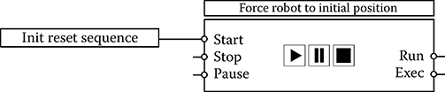
FIGURE 18.11 Block for generating signal patterns over time.
18.3.4.1.2 Rudimentary Support of Events
To describe dynamic systems that are driven by events, automation engineers use graphical tools based on the FSM formalism. Defined in the IEC 1131 standard, a language called sequential function chart allows programming of preferably linear chains of discrete steps. In addition to this, Winmod provides a tool to generate signal sequences over time (pattern generation, Figure 18.11). The sequence is defined with a simple text code and the graphical representation has an input to start the sequence. We used this feature to overrule the behavior of the machine model for initialization. This step beyond the physical reality is difficult, since the virtual machine is under the supervision of the actual controller, and error conditions must be avoided. The third possibility to handle events is a library of basic logic elements such as flip flops. All these state-oriented components run within the discrete time system and there is no separate discrete event control.
18.3.4.1.3 Graphical Programming
Since engineers prefer graphical descriptions, a representation similar to electric or electronic circuitry is provided. In UML 2.0, this corresponds to the communication diagram.
18.3.4.1.4 Object Creation by Composition
Object orientation is an essential concept for all kinds of software systems. Here it is preferred that new objects can be constructed only by combining objects, all derived from classes in a framework library. Some advanced concepts, such as multiple inheritance and object creation during runtime, are not allowed.
18.3.4.1.5 Import of Variables
The most powerful feature of a tool designated for machinery simulation is the capability to import variables, inputs, and outputs of the control system directly from its source code. This saves the work to define more than five hundred items for the actual project.
18.3.4.2 Example Details
The program code is a file of graphical drawings, consisting of blocks connected with signal lines (objects and message exchange in software terms). Here two important artifacts from Figure 18.6 are explained.
18.3.4.2.1 Integrator as Drive Design Pattern
All drives and subassemblies are modeled with first-order behavior (see Figure 18.12). This makes the basic numerical integrator to a design pattern for these artifacts (left). More complex drives are composed of several blocks but always have a similar representation (see Figure 18.12, right).
FIGURE 18.12 Simple drive modeled with integrator (left side); a more complex drive (right).
18.3.4.2.2 Exception Generator
During a training session, the trainee should resolve exceptional situations. For this reason, faults should be generated, for example, by blocking a cylinder or stalling a signal due to a broken sensor. The trainer may enter a number to select a predefined fault situation. The fault is triggered when the controller (and together with it, the entire plant) is in a certain state (see Figure 18.8). If the trainee is working alone on the simulator without a trainer, one fault out of a predefined list may be triggered at random. Of course, training without exeption is also possible.
18.4 Experiences With Simulation-Based Training
A training simulator was developed for the roll replacement procedure in a steel rolling mill. During a test period of several months, the effect of the training was observed. The most important criterion for the success of a training simulator is the acceptance by the personnel, which was excellent in the actual project. Periodic training sessions were carried out using the equipment since its introduction. After a period of some months, the following benefits became apparent and showed that the simulator meets expectations:
More training can take place than on the physical machine that is dedicated to production.
Training sessions can take place in a planned manner at scheduled times and not at arbitrary times during a production stop.
Training sessions on the simulator reduce the risk of damage to the physical machine.
The training program is standardized and contains all essential exercises. In contrast, on the deployed machine, seldom are all desired functions operable at one time.
Operators act faster and more accurate after being trained on the simulator. Resuming production after a fault is faster than before the introduction of the simulator.
Sometimes the cause of a failure in the complex system remains unclear. Simulation allows experimental repetitions to find the cause of such errors.
New components of the control software can be tested on the simulator before their implementation on the controller of the deployed machine.
The simulator helps in understanding the functions of the control system. It can also be applied for training of control engineers.
Software bugs in the actual control program were found, even severe ones.
Minor mistakes in the HMI could be detected, for example, wrong labels or swapped signals.
References
1. Pfeiler, H., N. Köck, J. Schröder, and L. Maestrutti. 2003. “The New Rail Mill of Voestalpine Schienen at Donawitz.” MPT International 26 (6): 40–4.
2. Page, R. L. 2000. “Brief History of Fligth Simulation.” In SimTecT 2000 Proceedings, pp. 11–7. Sydney.
3. Perkins, T. 1985. “Simulation Technology in Operator Training. Full-Scope Plant-Specific Simulators Are Part of the New Reality.” IAEA Bulletin 27 (3): 18–24.
4. Freedman, P. 2000. “New Drill Jumbo Operator Training Simulator.” IEEE Canadian Review 34: 16–8.
5. Isermann, R., J. Schaffnit, and S. Sinsel. 1999. “Hardware-in-the:Loop Simulation for the Design and Testing of Engine-Control Systems.” Control Engineering Practice 7 (5): 643–53.
6. Resmerita, S., P. Derler, W. Pree, and K. Butts. 2012. “The Validator Tool Suite: Filling the Gap Between Conventional Software-in-the-Loop and Hardware-in-the-Loop Simulation Environments.” In Real-Time Simulation Technologies: Principles, Methodologies, and Applications, edited by K. Popovici, and P. J. Mosterman. Boca Raton, FL: CRC Press.
7. Shahidehpour, M., H. Yamin, and Z. Li. 2002. Market Operations in Electric Power Systems: Forecasting, Scheduling, and Risk Management. New York: John Wiley & Sons.
8. Haq, E., M. Rothleder, B. Moukaddem, S. Chowdhury, K. Abdul-Rahman, J. G. Frame, A. Mansingh, T. Teredesai, and N. Wang. 2009. “Use of a Grid Operator Training Simulator in Testing New Real-Time Market of California ISO.” In IEEE PES Power & Energy Society General Meeting, Calgery, Alberta, pp. 1–8.
9. Issenberg¸ S. B., W. C. McGaghie, E. R. Petrusa, L. D. Gordon, and R. J. Scalese. 2005. “Features and Uses of High-Fidelity Medical Simulations That Lead to Effective Learning: A BEME Systematic Review.” Medical Teacher 27: 10–28.
10. Hodgkinson, G. P., N. Daley, and R. Payne. 1995. “Knowledge of, and Attitudes towards, the Demographic Time Bomb.” International Journal of Manpower. An Interdisciplinary Journal on Human Resources, Management & Labour Economics 16 (8): 59–76.
11. Lieberman, B. A. 2003. “The Art of Modeling, Part I: Constructing an Analytical Framework.” Accessed July 3rd 2010. http://download.boulder.ibm.com/ibmdl/pub/software/dw/rationaledge/aug03/fmodelingbl.pdf.
12. Seidl, E., C. Spielmann, and G. Rath. June 2010. Personal Discussion. Andritz AG.
13. Lieberman, B. A. 2007. The Art of Software Modeling, pp. 17. Boca Raton: Auerbach Publications.
14. Rowell, D. and D. N. Wormley. 1997. System Dynamics: An Introduction. Upper Saddle River, NJ: Prentice-Hall.
15. Colgren, R. 2006. Basic MATLAB, Simulink And Stateflow. Reston, VA: AIAA American Institute of Aeronautics & Ast.
16. White, S. A., D. Miers, and L. Fischer. 2008. BPMN Modeling and Reference Guide—Understanding and Using BPMN. Lighthouse Pt, FL: Future Strategies.
17. Kopetz, H. 1997. Real-Time Systems: Design Principles for Distributed Embedded Applications. Netherlands: Kluwer Academic Publishers.
18. Kweon, S. K., K. G. Shin, and Q. Zheng. 1999. “Statistical Real-Time Communication over Ethernet for Manufacturing Automation Systems.” In Proceedings of the 5th IEEE Real-Time Technology and Applications Symposium, pp. 192–202. Vancouver, Canada.
19. Winmod. “Real Time Simulation Center for Automation.” Accessed July 10th 2010. http://www.winmod.de.
20. Rosen, A. 2009. E-learning 2.0: Proven Practices and Emerging Technologies to Achieve Results. New York: Amacom.
21. Sauvé, L., L. Renaud, D. Kaufman, and J. S. Marquis. 2007. “Distinguishing between Games and Simulations: A Systematic Review.” Journal of Educational Technology & Society 10 (3): 247–56.
22. Garris, R., R. Ahlers, and J. E. Driskell. “Games, Motivation and Learning: A Research and Practice Model.” Simulation and Gaming 33 (4): 441–67.
23. Kickmeier-Rust, M. D. 2009. “Talking Digital Educational Games.” In Proceedings of the 1st International Open Workshop on Intelligent Personalization and Adaptation in Digital Educational Games, pp. 55–66. Graz, Austria.
24. Pannese, L. and M. Carlesi. 2007. “Games and Learning Come Together to Maximise Effectiveness: The Challenge of Bridging the Gap.” British Journal of Educational Technology 38 (3): 438–54.
25. Schiffler, A. 2006. “A Heuristic Taxonomy of Computer Games.” Accessed June 10th 2010. http://www.ferzkopp.net/joomla/content/view/77/15/.
26. McShaffry, M. 2009. Game Coding Complete. Boston: Course Technology.
27. Dalmau, D. S.-C. 2003. Core Techniques and Algorithms in Game Programming. Indianapolis, IN: New Riders Publishing.
28. Rehmann, A. J. and M. C. Reynolds. 1995. A Handbook of Flight Simulation Fidelity Requirements for Human Factors Research. Technical report, CSERIAC. Springfield, Virginia: National Technical Information Service.
29. Klatt, K.-U. 2009. Trainingssimulation. ATP 51 (1): 66–71.
30. Mewes, J. and G. Rath. July 2010. Personal Discussion, CEO of Mewes & Partner, Berlin.
31. Bullinger, H.-J. and J. Warschat. 1996. Concurrent Simultaneous Engineering Systems. London: Springer.
32. Parr, E. A. 2003. Programmable Controllers: An Engineer’s Guide. 3rd ed. Oxford: Newnes.
33. Bolton, W. 2009. Programmable Controllers. 5th ed. Oxford: Newnes.
34. Lewis, R. W. 1996. Programming Industrial Control Systems Using IEC 1131-3. The Institution of Electrical Engineers.
35. MathWorks. 2010. “Simulink® PLC Coder™.” Accessed July 3rd 2010. http://www.mathworks.com/products/sl-plc-coder/
36. Pilone, D. and N. Pitman. 2005. UML 2.0 in a Nutshell. Cambridge, MA: OReilly & Associates.
37. Borel, É. 1913. “Statistical Mechanics and Irreversibility (Mécanique Statistique et Irréversibilité).” Journal of Physics (Journal of Physique.) 3 (5): 189–96.
38. Crosbie, R. 2012. “Real-Time Simulation Using Hybrid Models.” In Real-Time Simulation Technologies: Principles, Methodologies, and Applications, edited by K. Popovici, and P. J. Mosterman. Boca Raton, FL: CRC Press.
39. Hodgson, J., R. Hyde, and S. Sharma. 2012. “Systematic Derivation of Hybrid System Models for Hydraulic Systems.” In Real-Time Simulation Technologies: Principles, Methodologies, and Applications, edited by K. Popovici, and P. J. Mosterman. Boca Raton, FL: CRC Press.