
22 Modelica as a Platform for Real-Time Simulation
John J. Batteh, Michael M. Tiller and Dietmar Winkler
CONTENTS
22.1 Introduction
With the growing adoption of model-based system development to shorten product development cycles and reduce costs and hardware prototypes, modeling of physical and control systems has emerged as a critical element in modern systems engineering efforts. The systems engineering V is a standard way to describe the processes that encompass a system engineering effort. While the V model has been refined as applied in particular industries, the core process steps are largely similar across applications. One representation of the systems engineering V as applied to intelligent transportation systems is shown in Figure 22.1. Modeling and simulation supports the systems engineering V throughout the entire product development process. In the early stages of the V, upfront modeling supports initial concept assessment and target and requirements cascade moving down the left side of the V. Computer-aided engineering (CAE) methods such as finite element analysis (FEA) and computational fluid dynamics (CFD) are typically employed at the bottom of the V to support detailed design and development efforts. Moving back up the right side of the V, the integration and verification phases routinely involve verification and validation (V&V) using model-based representations of the engineered system. After system deployment, models can be used to help understand and diagnose issues in the field and can even provide simulation-based maintenance opportunities. Although the type of modeling naturally evolves with engineering tasks and data availability throughout the product development process, it is quite clear that models can and do play a critical role in complex systems engineering efforts.
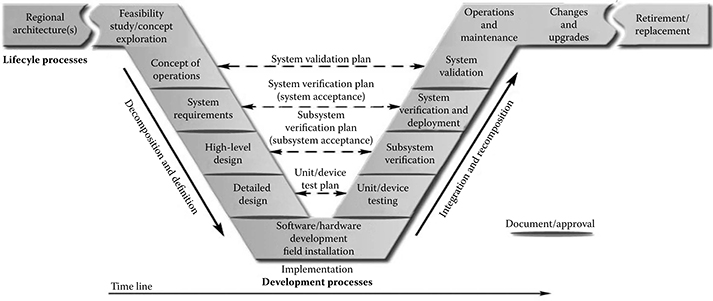
FIGURE 22.1 Systems engineering V. (From National ITS Architecture Team, Systems Engineering for Intelligent Transportation Systems, Report no. FHWA-HOP-07-069, United States Department of Transportation, 2007, http://www.ops.fhwa.dot.gov/publications/seitsguide/index.htm (accessed June 30, 2010). With permission.)
While upstream modeling efforts may be wholly contained in the virtual realm, the necessity to integrate models with hardware increases during the later stages of the product development process as virtual prototypes are replaced by their physical representations. Computational efficiency becomes a key issue during this stage of the integration as models must simulate in real time to satisfy hardware interface requirements. Satisfying real-time simulation constraints is often one of the most challenging tasks for model developers. Making appropriate trade-offs between model complexity and model fidelity requires keen understanding of the underlying system dynamics and the spectrum of time scales inherent in the modeled system and input drivers.
This chapter introduces the modeling language Modelica [1] as a modeling platform to support real-time simulations. A brief introduction to the Modelica language and its fundamental language features will be given. The focus of this work is on the features of the Modelica language that make it desirable for modeling of physical systems for real-time targets. While the Modelica language itself is open and can be interpreted by a wide variety of free and commercial tools [54] for potential generation of real-time executables, the intent is not to focus on any particular tool or application but rather the language itself.
22.2 Modelica Overview
Modelica is a nonproprietary, object-oriented modeling language for multidomain physical systems. Models in Modelica are described by differential, algebraic, and discrete equations. Modelica has been used to model a wide variety of complex physical systems in the mechanical, electrical, thermal, hydraulic, pneumatic, and fluid domains with significant industrial application in the aerospace, automotive, and process industries. An extensive list of publications, including the full proceedings from all Modelica conferences, is available on the publication page of the Modelica website [2]. As a complement to modeling of acausal physical behavior, Modelica also supports modeling of systems with prescribed input/output (I/O) relationships (i.e., causal systems), such as control systems and hierarchical state machines. This section gives a brief overview of the Modelica language and its fundamental language features.
22.2.1 History
The Modelica language has evolved as a collaboration between computer scientists and engineers to provide a modeling language to describe the behavior of multi-domain physical systems in an open format not tied to a particular tool. The roots of the Modelica language can be traced back to Hilding Elmqvist’s PhD thesis [3] in which he designed and implemented the Dymola modeling language. The Dymola language used an object-oriented, equation-based approach to formulate models of physical systems. Rather than forcing modelers to pose the problem using ordinary differential equations (ODEs) for which many solvers exist, the Dymola language allowed the problem to be posed as differential-algebraic equations (DAEs), which is generally considered a more natural way to describe physical problems [4]. Sophisticated symbolic algorithms were used in the language implementation to transform the mathematical model into a form capable of solution by existing numerical solvers. As symbolic algorithms advanced, in particular, the Pantelides algorithm [5] for DAE index reduction, it became possible to solve an even larger class of problems using the new approach pioneered by the Dymola language. Within the context of the ESPRIT project “Simulation in Europe Basic Research Working Group (SiE-WG),” Hilding Elmqvist in 1996 sought to bring together a group of object-oriented modeling language developers and engineering simulation experts in an attempt to develop a new modeling language to describe physical systems over a wide range of engineering domains. After a series of 19 meetings over the course of the next 3 years, version 1.3 of the Modelica language specification was released in December 1999.
The Modelica language specification is maintained by the Modelica Association, a nonprofit, nongovernmental organization established in 2000. The Modelica Association consists of individual and organizational members who actively participate in the design of the Modelica language. Since the initial release of the language specification, several major updates to the language have been released that incorporate additional language elements. The current version of the Modelica specification is version 3.2 [1]. The current and the previous versions of the Modelica specification are available on the Modelica website [6]. In addition to the Modelica language specification, the Modelica Association also develops and maintains the Modelica Standard Library (MSL), a large, free, multidomain library of Modelica models. The MSL serves as a common link between free and commercial library developers to promote compatibility between implementations. A listing of free and commercial libraries is available on the libraries page of the Modelica website [7]. For more history on the Modelica language, the interested reader is referred to the two published books on the language [8,9]. The most current information on the Modelica language can be found on the Modelica website at www.modelica.org [10].
22.2.2 Modelica Example
To illustrate a few key features of the Modelica language, consider the example shown in Figure 22.2. This multiphysics model consists of a battery connected to a motor driving a load. The battery model includes the heat-generation effects of the dissipative resistance and the resulting degradation in voltage due to thermal effects. The thermal network model includes a lumped model of the battery thermal mass along with simple flow-based cooling through convection. A controller controls the battery cooling by monitoring the battery temperature and actuating the flow rate in the cooling system to achieve the desired battery temperature. This multidomain physical system model contains elements from the mechanical (rotational), electrical, and thermal domains. The model was constructed both from component models in the MSL and from models implemented by the authors.
The Modelica source code for the example model is shown in Figure 22.3. The Modelica source code completely describes the dynamics of the system, but a compiler is necessary to actually simulate the example. As will be described later in this chapter in more detail, the compiler flattens the equations in the Modelica source code and combines them into a causal set from which computer code can be generated for integration with existing numerical solvers.
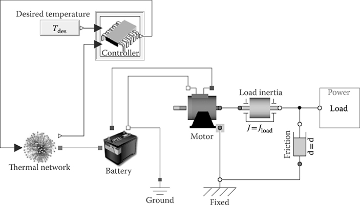
FIGURE 22.2 Modelica example model.
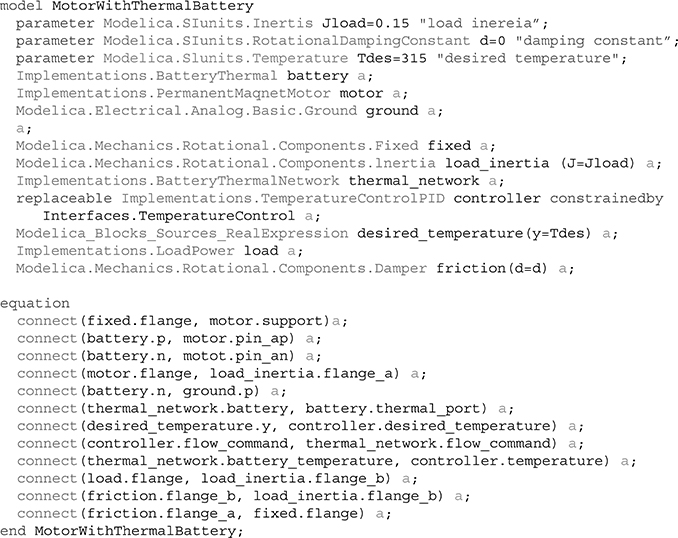
FIGURE 22.3 Modelica code for example model.
To provide further understanding of the dynamics of the model, Figure 22.4 shows simulation results as generated by the commercial tool Dymola* [11]. The load applied to the system is shown along with the resulting battery terminal voltage, battery temperature, and the controlled flow command for battery cooling. Note that the cooling system has a fixed cooling capacity that is insufficient to maintain the battery temperature under high-load conditions. Since the battery voltage is a function of the temperature, the desired load power is not met under all conditions. This example model will be used in Sections 22.3.4 and 22.3.5 to illustrate key concepts related to real-time modeling capability and model configuration.
A key language feature in Modelica is the connector concept. Connectors are used to define the interfaces of the models. A unique connector is defined once for each physical domain. A connector definition primarily consists of two kinds of variables: a potential variable and a flow variable. These variables can also be described as “across and through” or “effort and flow” variables. Special semantics apply to connections made between connectors, and such connections result in equations between variables in the connectors. In a connection set, all matching potential variables are equated, and all matching flow variables are summed to zero at the connection point. Referring to the example model in Figure 22.2, the rotational connectors are depicted as gray circles, the electrical connectors as blue squares, and the thermal connectors as red squares connected between the battery and the thermal network components. The definitions of the connectors from the MSL are shown in Figure 22.5.
* Dymola was used to generate all simulation results shown throughout this work though nearly any Modelica-compliant tool could have been used.
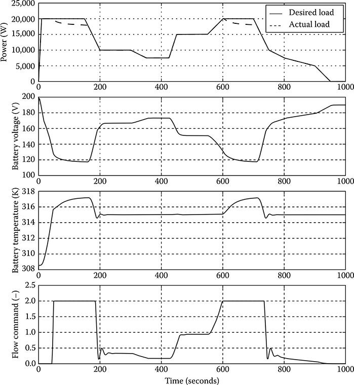
FIGURE 22.4 Sample simulation results from the motor battery example.
The connector concept is extremely powerful as it facilitates natural, acausal modeling of physical systems where connections between components in the Modelica model mimic connections seen in the physical world. As will be discussed in more detail, acausal models include no a priori assumptions about causality and allow quick and effortless model construction and reconfiguration. For example, a connection between rotational connectors is equivalent to a rigid connection (i.e., a kinematic constraint or an inertialess shaft) between physical elements. In the electrical domain, a connection between components is equivalent to a lossless wire connection (i.e., a perfect short). Just as physical systems are constructed through connections between hardware components, Modelica models are constructed through connections between equivalent virtual components. In this way, the virtual representation is consistent with system design schematics used by engineers.
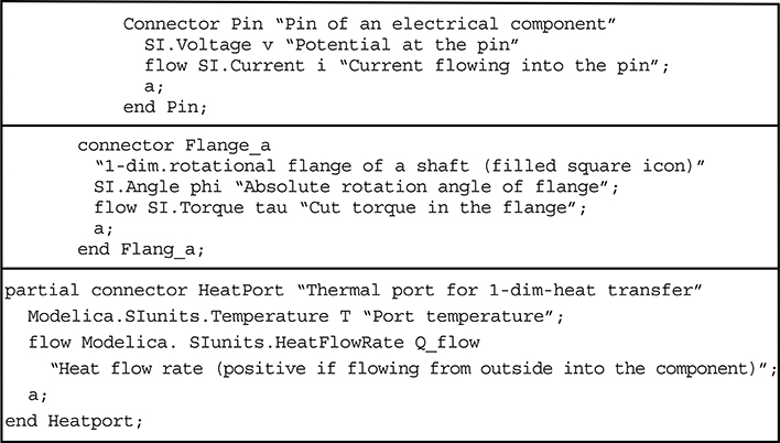
FIGURE 22.5 Connector definitions.
Another key feature of the connector-based approach is the ability to seamlessly integrate models from various sources. The use of the standard connectors defined in the MSL ensures model compatibility between the MSL, user-implemented, free, and commercial libraries. Thus, Modelica with its open language specification is also an ideal model exchange format. As mentioned previously, the example model in Figure 22.2 consists primarily of models from the MSL. At the top level of the model, the motor, damper, and inertia components are from the MSL. The thermal network, battery, load, and controller were primarily implemented as subsystems constructed from lower-level components of the MSL. The thermal network subsystem model is shown in Figure 22.6. The only author-implemented model in the thermal network is the component that calculates the heat transfer coefficient for the convection element based on the cooling flow rate. With established multidomain connectors, model implementations using those connectors in the MSL, and other core language features to promote model reuse and configurability, the Modelica language provides a powerful platform for model-based systems engineering.
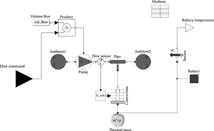
FIGURE 22.6 Thermal network subsystem from example model.
22.3 Modelica Features
With that brief introduction to the Modelica language, this section elaborates more specifically on Modelica language features and associated attributes that make Modelica a desirable platform for real-time simulation. The focus will be primarily on Modelica although a few tool-specific implementations relative to real-time simulation capability are briefly discussed.
22.3.1 Open Platform
Modelica is a nonproprietary language and thus offers an open platform for model and application development. The nonproprietary nature of the language allows intellectual property captured in models to be maintained separate from the tools thereby allowing model developers to move freely among Modelica-capable tools based on their relative merits. This situation is in stark contrast to other simulation tools where the models are integrated with the tools in a proprietary way and thus are not portable to other tools. While conformance to the same language syntax allows tool-independent model formulation, it should be noted that simulating the same model identically between tools also requires that the execution engine is formalized and used as reference semantics for each of the tools.
Another opportunity that arises from the open platform is that of accessibility. Since the Modelica specification is open and freely available, any interested party is welcome to create a parser and even a compiler to interpret Modelica source code. With source code for many solvers already available, it is certainly feasible to create custom tools for Modelica model development and simulation. For example, the Modelica Software Development Kit (SDK) [12] provides an API and Modelica compiler to allow Modelica code to be embedded into existing software and tools. The open platform also supports innovation from small companies and universities. Several open-source, Modelica-based projects have been initiated. OpenModelica [13] is an open-source Modelica modeling and simulation environment. JModelica.org [14] is an open-source Modelica-based platform for simulation and optimization. Scicos [15] developed at INRIA is a modeling and simulation environment that includes partial support for Modelica. While these offerings may not be as comprehensive in their support of the Modelica language as existing commercial tools, they certainly illustrate potential for innovative offerings based on the open Modelica platform.
Besides accessibility to the Modelica language for custom tool development, another benefit of the open platform is the large quantity of high-quality models that are available in the MSL and free Modelica libraries. Rather than working on simplified, academic problems, the existing Modelica model base provides high-quality, relevant models in multiple engineering domains that can be used to fully support tool and algorithm development. These models allow tool and algorithm innovators to work on real technical problems with models that are already available thus reducing the burden of creating complex examples to showcase new algorithm or tool capabilities.
22.3.2 Acausal Modeling
Modelica supports two of the most common modeling formalisms for continuous systems: block diagram and acausal modeling [8]. The block diagram approach involves constructing systems of component blocks to calculate unknown quantities from known quantities. The block diagram, or causal, approach is very well suited to modeling of controllers where the signal flow concept is quite natural. The sensor signals are known inputs, and the controller model is responsible for calculating actuation signals based on the sensed signals. The block diagram approach is not as well suited to physical system modeling in which the relevant mathematical description for the behavioral dynamics consists of conservation equations. For example, what would be the “input” to a resistor?
Acausal modeling involves modeling components from a free body or first principles sense without a priori assumptions about I/O causality. Acausal models specify relationships in which potentials across components drive flow of conserved quantities. Physical components are naturally acausal and are naturally described by the Modelica connector-based approach. Figure 22.7 shows an example of a mechanical system modeled with both acausal and block diagram formalisms in Modelica. For those familiar with the physical system schematics, the acausal representation is a natural virtual representation. Furthermore, the acausal component models can be reused regardless of the causality imposed by the system while the implementation of the block diagram model changes drastically because of fundamental changes in the inputs and thus the model structure.
Another benefit of the acausal modeling formalism as implemented in Modelica is that components can generally be connected in a physical way without restriction. This feature has a profound impact both on model management and configuration and on model computational efficiency, a critical factor in real-time simulation. One of the key challenges in real-time simulations is striking a balance between model fidelity and computational expense. To achieve this balance, idealizations to improve performance are often required.
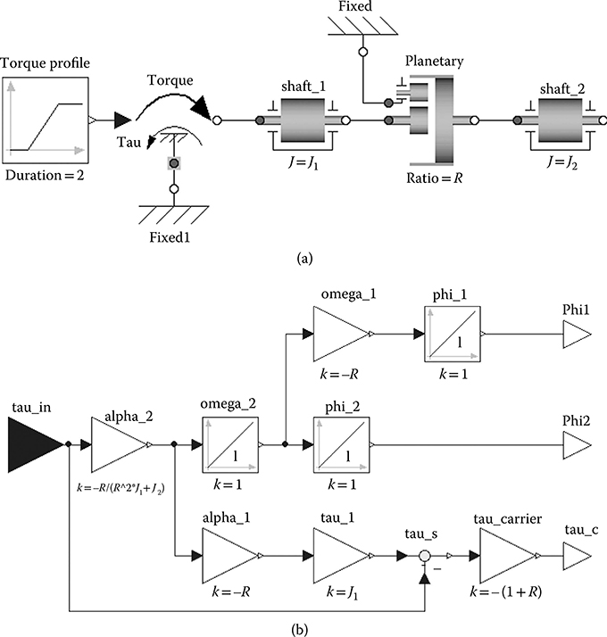
FIGURE 22.7 Sample model in (a) acausal and (b) block diagram formalisms.
To illustrate this point, a vehicle modeling example is considered. There are many compliant elements in a vehicle drivetrain, and these elements can lead to significant noise, vibration, and harshness (NVH) issues in the driveline as excited under various driving conditions. Capturing the NVH effects in the drive-line necessitates the modeling of the key compliances in the system and results in higher-order dynamics in the vehicle drivetrain. These higher-order dynamics are, in fact, the focus of the NVH modeling effort. In addition to the NVH model, another class of vehicle models is focused on the simulation of vehicle performance and fuel economy. Performance and fuel economy models are typically simulated over long time scales, including drive cycles that can be thousands of seconds in length. On this time scale, the higher-frequency NVH effects do not typically impact the vehicle-level results significantly. Thus, the idealization of the drivetrain as rigid is a perfectly reasonable assumption for a performance and fuel economy model.
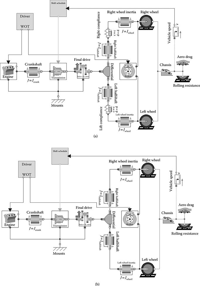
FIGURE 22.8 Simplified vehicle models with a (a) compliant and (b) rigid drivetrain.
To illustrate the two classes of vehicle models, consider Figure 22.8, which shows a simplified vehicle model with a compliant and rigid drivetrain. The two models are identical save for the spring-damper element that represents the compliance of the half shafts. Note that the rigid model actually has two inertia elements connected together representing the wheel and half shaft inertias. While many physical modeling tools have difficulties with such configurations (because they lead to high-index DAEs), this is not the case in Modelica, which was designed with high-index systems in mind. Connecting two inertias together might seem odd, especially in a flat model such as the ones shown in Figure 22.8. This topic will be addressed shortly as part of the configuration management discussion.
Now consider the situation where the compliant model is used for performance and fuel economy simulations, perhaps because of limitations in the modeling tool to handle rigid, kinematic connections. In an attempt to stiffen the compliant model to mimic the behavior of a truly rigid model, the stiffness of the compliant element is increased. Figure 22.9 shows simulation results from a wide open throttle (WOT) simulation of the rigid and compliant vehicle model. The stiffness of the compliant vehicle model has been set to roughly twice the typical half shaft stiffness to approach the behavior of the rigid model. The vehicle-level behavior of the two models is nearly identical as can be seen from the vehicle speed and the engine speed comparisons. However, the computational expense is nearly twice as great for the compliant model as illustrated by the CPU time required for the simulation. In particular, note the jumps in CPU time corresponding to each shift event in the compliant model. While this evaluation was performed with an open loop WOT test to try and isolate the compliant effects, it should be noted also that the WOT simulation is not nearly as dynamic as a drive cycle where the driver inputs could be changing much more rapidly thus introducing even more shift events and likely resulting in even larger differences in simulation time between the compliant and the rigid models.
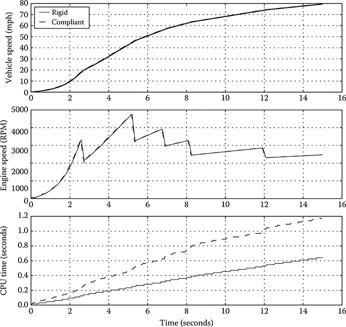
FIGURE 22.9 Simulation results from rigid and compliant vehicle model.
While the simple vehicle model shown in Figure 22.8 modeled the drivetrain in a flat fashion at the top level of the model without introducing another level of hierarchy, this modeling approach was primarily used to make it easier to illustrate the differences between the rigid and the compliant models. In fact, even this simple model includes enough components and connections that the top level of the model is becoming crowded and would benefit in terms of readability from the grouping of additional components into logical subsystems. As mentioned previously, it may seem that the potential need for the compliant element in the vehicle model is an artifact of the modeling of the half shaft and wheel as two separate inertias instead of a single effective inertia. While it is easy to see the two inertias connected together in the flat model, it would not be as obvious if the two inertias were part of separate subsystems.
Another benefit of grouping components into subsystems is to take advantage of an architecture-based modeling and model configuration approach. This topic will be discussed in more detail later in this chapter. An architecture-based modeling approach hinges on the ability to arbitrarily connect components. If the modeling tool cannot handle arbitrarily connected components, one remedy for the underlying conflict between the configuration management and the model mathematics is to insert unphysical interfaces, such as stiff springs in a mechanical system to ensure that the two inertias are not connected together, at the expense of computational efficiency. With no restrictions on component connections in Modelica, Modelica can support architecture-based model configuration while maintaining the natural physical interfaces between components, even if those interfaces include rigid connections.
22.3.3 Symbolic Manipulation
While acausal models are clearly preferable to block diagram implementations for physical systems modeling, acausal models do introduce simulation challenges. While ODEs are convenient to solve, most physical problems in science and engineering are naturally described by DAEs. Acausal models require the solution of DAEs that include both ODEs and algebraic equations representing the system constraints. The efficient solution of DAEs, particularly high-index DAEs that result from structurally singular systems that have constraints between states, requires a combination of symbolic and numerical approaches and is an active research topic. The Modelica language has been designed to specifically protect for these approaches and optimizations to support the generation of efficient code from DAEs.
While Modelica provides the language to allow the expression of mathematical models, it does not prescribe the method for solving the resulting DAEs. The solution method and solver integration falls into the realm of the Modelica compiler, be it commercial or open source as described previously. This section briefly describes some of the symbolic and numerical techniques used in the solution of DAEs. The intent is not to focus on the algorithms or techniques but is instead to focus on the Modelica language elements that support them. The interested reader is referred to the works by Cellier et al. [4], Cellier and Kofman [16], Celier [53], and Anderson [17] for more details on the algorithms and numerical techniques briefly introduced here.
The mathematical description of models in Modelica consists of Boolean, discrete, and DAEs. On the basis of a Modelica model, the resulting set of Boolean equations, discrete equations, and DAEs can be obtained. However, there are no general-purpose solvers for these sets of equations. Direct numerical DAE solvers typically result in slow simulations. The standard approach in Modelica-based tools is to translate the DAE into an ODE form for solution. Since a Modelica model preserves the equations that describe the relationships between variables in symbolic form, it is possible to perform symbolic analysis and manipulation to aid in the solution of the resulting set of equations. Symbolic analysis helps determine an efficient way to develop a causal set of equations that can be solved numerically or even symbolically if possible.
To generate a causal set of equations, the first task is to understand the structure of the problem. One way to understand the problem structure is through a structure incidence matrix [16,17]. The rows of the matrix are indexed by the equations and the columns by the variables or unknowns. If an equation contains a given variable, the number one is placed in the corresponding entry in the matrix. Using the information provided in the matrix, a rule-based approach can be used to determine which variable should be solved from each equation. Another method to generate a causal set of equations is an algorithm based on graph theory and first proposed by Tarjan [18]. In this method, a structure digraph shows the equations and unknowns as nodes in vertical columns with lines drawn between nodes if an unknown appears in a given equation. On the basis of the information in the structured digraph, the algorithm defines an approach that can sort the equations into a causal, executable sequence. The resulting equivalent structure incidence matrix is lower triangular, and therefore, there is an equation to compute each of the unknowns from variables that have already been computed. The Pantelides algorithm [5] is a popular causalization algorithm because of its compact recursive implementation [16].
While equation sorting is a key component in the solving of DAEs, it is not entirely sufficient for full triangularization, in particular, in case of cyclic dependencies between variables, or so-called algebraic loops. Instead of a true lower triangular incidence matrix, the sorting algorithms result in block lower triangular form with the blocks containing the equations that are part of the algebraic loops. Depending on the nature of the problem, the loop equations could be either linear or nonlinear, and there are many techniques to solve the resulting equations. Blocks containing linear equations can be solved efficiently (and symbolically if they are small enough), but nonlinear equations will generally require Newton iterations.
An approach that has a profound impact on computational efficiency for algebraic loops is tearing. A tearing algorithm seeks to break apart a system of equations by assuming values for variables and then solving the resulting set of equations with residual equations for the torn variables based on the system of equations. By analyzing the structure of the underlying system, it is possible to identify tearing variables that can have a drastic impact on computational efficiency [16]. Tearing often leads to a reduction in the number of iteration variables for solving the nonlinear equations. It may also result in significant decoupling of simultaneous systems of equations with the potential for more efficient solution of the decoupled equations based on the known value of the tearing variable.
A key element to computationally efficient modeling is the handling of events where logical expressions change value [16]. Event handling is especially important since discontinuous equations or changes in model behavior must be handled as discrete events for numerical integration schemes. Since the integration is typically interrupted to resolve each event, unnecessary events can severely hamper computational speed. Modelica includes language semantics to control the handling of events. The semantics of the smooth operator indicate to the Modelica compiler that an expression is continuously differentiable up to the order provided by the user [1]. Since the expression on which the smooth operator acts can involve complex branching constructs such as if statements, the smooth operator aids the Modelica compiler in identifying the structure of the problem regarding continuity of the variables and partial derivatives of the variables in the expression and potentially avoiding unnecessary events at branching conditions since the modeler has guaranteed continuity up to a particular order. The noEvent operator in Modelica is also used to avoid the generation of events by controlling the generation of crossing functions from complex expressions with branching conditions based on variables of type real [1].
As noted previously, minimizing the number and size of nonlinear equations that must be solved can also have a significant impact on computational efficiency. The semiLinear operator in Modelica is used to help the Modelica compiler identify situations where an expression is linear with respect to a given variable but with two different slopes when the variable is positive and negative [1]. This operator can help the compiler to generate sets of linear equations rather than nonlinear ones. The semi-Linear operator is symbolic in nature and gives the underlying tool a greater understanding of the modeler’s intent, which can help resolve some ambiguities in certain classes of models. One example of such semiLinear operator usage is in the handling of reversing flow in fluid systems where the flow enthalpy is either the upstream enthalpy or the downstream enthalpy based on the direction of mass flow [19].
Another example where symbolic information is very useful is in state selection. For acausal models, state selection is not trivial since variables introduced in completely different subsystems can end up being kinematically coupled through the connection graph. Therefore, it is necessary to symbolically analyze the entire model to identify such cases and resolve a unique set of states. Furthermore, the selection of appropriate states for integration can drastically affect computational efficiency. For example, the modeler might want to control the states that are selected as part of the symbolic manipulation process based on knowledge of the problem or details of the formulation. In thermodynamic problems, the conservation equations are written in terms of mass and energy, but it is typically preferable to select the intensive variables pressure and temperature as states rather than the extensive variables that depend on the size of the system and can vary greatly over a given simulation. Furthermore, consider that property relationships, such as enthalpy and internal energy, are often explicitly written as nonlinear functions of pressure and temperature, and any other state selection would require the solution of a nonlinear equation to determine the intensive variables. The Modelica language includes the stateSelect language element to help the modeler control the selection of states [1]. The stateSelect element also allows the modeler to exert varying degrees of control over the state selection. Using the stateSelect attribute, it is possible to specify that a given variable is always selected as a state, that it should be preferred as a state, that it should not have any preference with regard to state selection, that it should be avoided as a state, or, finally, that it should never be chosen as a state. The Modelica language even allows initial equations to be specified for variables that are not states. For example, in a thermodynamic system with mass and energy as states, pressure and temperature can be specified for initialization. Another example of the impact of state selection on computational efficiency is in three phase electrical systems where the dq0 or Park transformation [20] can be applied to calculate alternative currents that exhibit more DC-like behavior. The choice of the alternative currents as states can drastically improve computational speed and can be easily achieved in Modelica using the stateSelect construct [21].
To illustrate the impact of equation sorting, state selection, and causality on computational efficiency, consider the following electrical example reproduced from the excellent tutorial by Bernhard Bachmann [21] on the mathematical aspects of object-oriented modeling. The model shown in Figure 22.10 is a simple electrical circuit consisting of sinusoidal voltage source, inductor, and a nonlinear resistor implementation. Two equivalent models are formulated for the nonlinear resistor with i = f(v) causality as shown in Equation 22.1 and v = f(i) causality as shown in Equation 22.2:
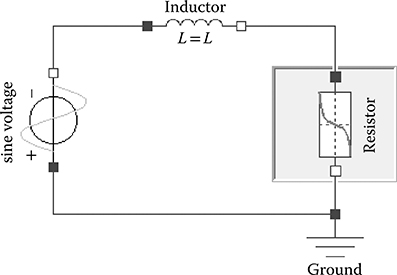
FIGURE 22.10 Electrical example model with nonlinear resistor.
FIGURE 22.11 shows the simulation results from the circuit with the two resistor implementations. The voltage and the current in the resistor are identical as expected, but the computational expense is significantly higher for the i = f(v) formulation. The explanation for this effect is a result of the interaction between the state selection and the causality of the nonlinear equation. For this model, the typical state selection where differentiated variables are automatically chosen as states results in the current as a state. With the i = f(v) causality, a nonlinear equation must be solved to determine the voltage drop across the resistor. With the v = f(i) causality, a solution of nonlinear equations is not required as the nonlinear equation can simply be evaluated for the voltage drop. Bachmann [21] notes that the causality that results in the most efficient solution depends on the model topology. If the inductor and the resistor were placed in parallel rather than in series as in Figure 22.10, then the i = f(v) implementation would be the more efficient formulation. This example also highlights why it is so important to have symbolic model representations where the formulation details are visible such that these issues can be diagnosed and understood.
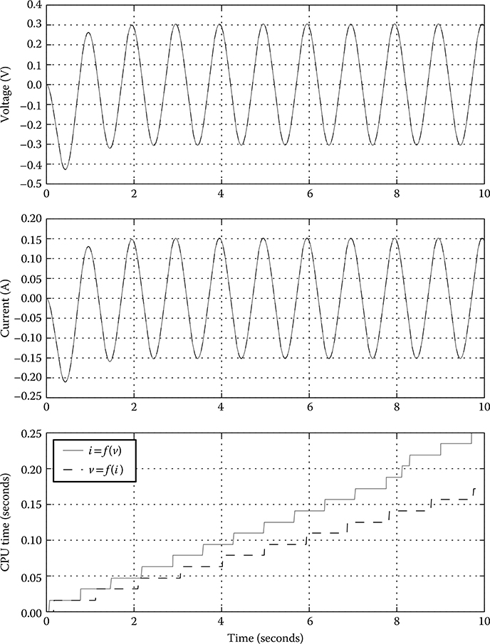
FIGURE 22.11 Simulation results from electrical example with nonlinear resistor.
22.3.4 Inverse Models
Another benefit of acausal modeling is the support for inverse models. An inverse model is formulated by specifying model outputs rather than model inputs. The resulting executable model must then calculate the model inputs such that the model outputs are as prescribed. Causality is reversed in an inverse model since outputs are known and inputs are unknown thus requiring an acausal model formulation. Inverse models are sometimes denoted as backward models as opposed to forward models that are conventionally driven with known or calculated inputs. Inverse models can be used in place of controller logic to support rapid, upfront design concept assessment and feasibility without requiring a detailed controller design and tuning effort that would otherwise be required to reasonably assess the concept design [22]. Inverse models are also extremely useful for providing insight into control system design. A few examples of inverse modeling with Modelica involve the formulation of driver models that perfectly follow a prescribed vehicle speed trace for powertrain simulations [23], energy consumption studies in aircraft equipment systems in response to prescribed load traces [24], and model-embedded control applications [22].
Inverse modeling approaches can also be used to impact computational efficiency. Inverse models can be used to implement perfect control in lieu of proportional– integral–derivative (PID) controller implementations with high gains. While high gains can improve the ability of the system to follow a desired trace, significant tuning is often required to achieve desired control response. A side effect of high gains is the introduction of high-frequency inputs that can excite high-frequency response in the model thus affecting computational efficiency. The situation is especially acute if the high-frequency response is beyond the bandwidth of interest for the simulation. Ultimately, however, the high-gain implementation is simply trying to mimic the perfect control response.
Inverse models can also be used to implement localized perfect control in the context of a complex control architecture where a particular control feature is replaced by a perfect control implementation. One can imagine this model inversion acting as a sort of “perfect control,” which, assuming the system is sufficiently invertible, ensures that the desired response is exactly achieved. By implementing perfect control, one or more states in the model can typically be removed thus reducing the total number of states in the system as well as potentially eliminating eigenmodes that slow down the integration as well. Reduction in the number of states is especially useful for model embedded control applications where the computational expense grows nonlinearly with the number of states in the system [22]. It should be noted that, depending on the linearity of the model being controlled, perfect control can result in nonlinear systems that were not present in the forward facing model. The ability of a Modelica compiler to tear nonlinear systems is the key to minimizing the impact of nonlinear systems generated by a perfect control approach. If the nonlinear systems are too extensive or prove difficult to solve, it is certainly possible that the computational efficiency of the perfect control approach could be degraded compared to the forward facing implementation. The trade-off between nonlinear systems and more states with potentially linear systems must be evaluated on a per problem basis.
As an illustration of perfect control in Modelica, consider again the model shown in Figure 22.2. Figure 22.12 shows the original controller implementation with a PID controller and also a perfect control implementation. Note that the PID controller has been replaced by a block from the MSL to handle inverse problems. Simulations were conducted by simply replacing the original controller with the perfect controller using the Modelica language features for model configuration. Figure 22.13 shows results from running the simulation with the perfect control. The flow command limits have been removed to illustrate the commands issued by the perfect controller to achieve the desired battery temperature. With perfect temperature control, the system can also meet the desired load command. It should be noted that the unconstrained perfect control simulation yields the dynamic range necessary by the controller to achieve the desired output response. Thus, the results are not identical to those in Figure 22.4 using the PID controller for which the flow command was limited. Note, however, that there is evidence of some oscillatory behavior in the flow command signal from the PID controller implementation in Figure 22.4. For this sample problem, no effort was expended to tune the controller to potentially reduce or eliminate the oscillatory commands for the PID implementation; obviously, no tuning is required for the perfect control implementation to identically achieve the desired target.
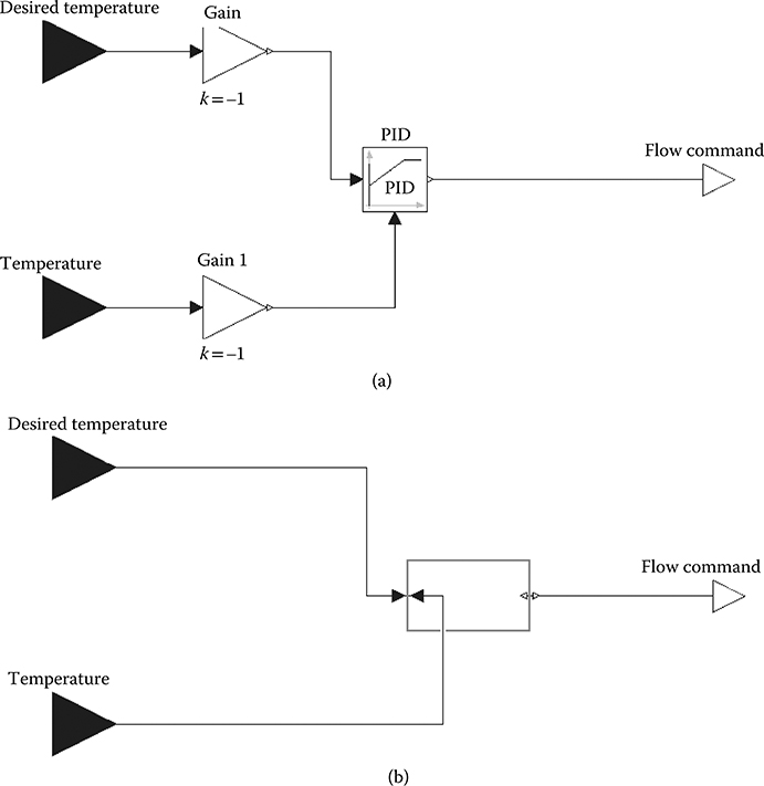
FIGURE 22.12 PID (a) and perfect control (b) temperature implementations.
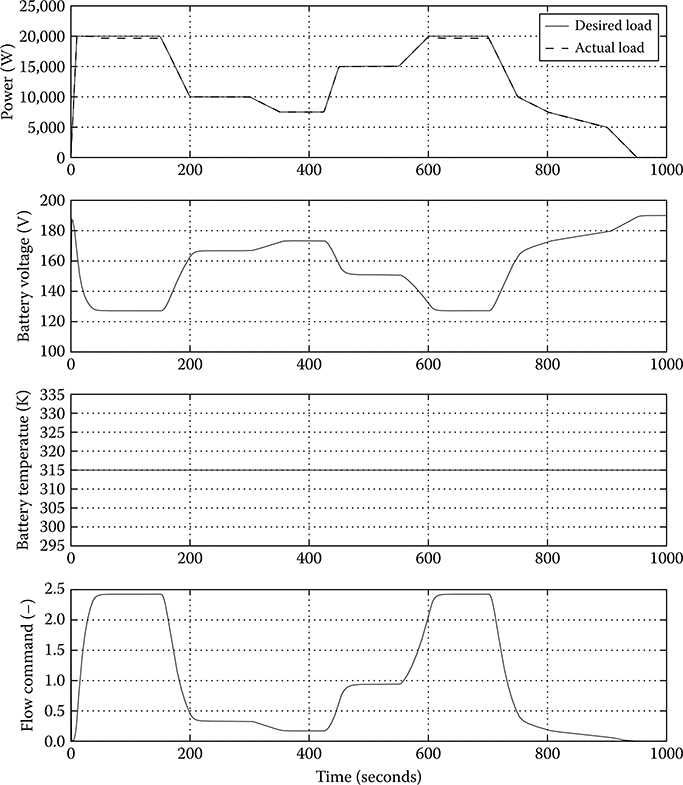
FIGURE 22.13 Sample simulation results from the motor battery example with perfect controller.
22.3.5 Model Configuration
With a distributed, acausal model development approach, system models are constructed through connections between component or subsystem models. While it is possible to assess model fidelity with testing at the component and subsystem level, the impact of individual model implementations on computational efficiency is often not revealed until the system model is assembled and tested. As models transition from desktop simulations to real-time platforms, variants of individual models may be required to support real-time execution.
Model configuration and variant management are key components of effective model management for any model-based systems development effort. The Modelica language includes several language features that directly support model configuration. To support plug-and-play model configuration, the Modelica language allows configuration management through the replaceable language construct. The replaceable semantics allow model variants to be created by replacing individual models with other compatible models. With a strong typing system, compatible models can be easily identified. Returning to the motor battery example, consider the construction of the model with the perfect controller. The perfect controller model variant is constructed by replacing the original controller with the perfect controller (note the replaceable qualifier before the instantiation of the controller component in Figure 22.3). The Modelica code to create the model variant is shown in Figure 22.14. Since Modelica supports inheritance, the model variant is created by inheriting from the original model shown in Figure 22.3 and simply replacing the original controller implementation with the PID implementation. While this example illustrates configuration of a top-level model component, model configuration through the replaceable construct can occur at any level of the model hierarchy. The ability to create model variants without code duplication increases modeling efficiency and aids in effective model management. The replaceable construct allows plug-and-play configuration of different versions of the same model with selected model variants to support real-time applications.
As shown in the motor battery example, Modelica models can be easily constructed by connecting component models, and model variants can be created using the replaceable construct. The next level in model configuration management uses prewired model architectures of configurable components for plug-and-play construction of model variants. Figure 22.15 shows a sample model architecture to support vehicle system modeling [23]. Model architectures offer an even more powerful platform for managing model variants as many different applications can be supported with the same architecture. The same architecture can support models of varying levels of detail, a key feature for real-time modeling.
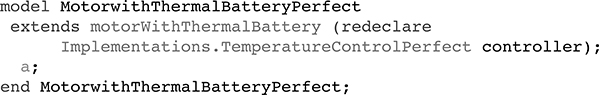
FIGURE 22.14 Modelica code for example model with perfect controller.
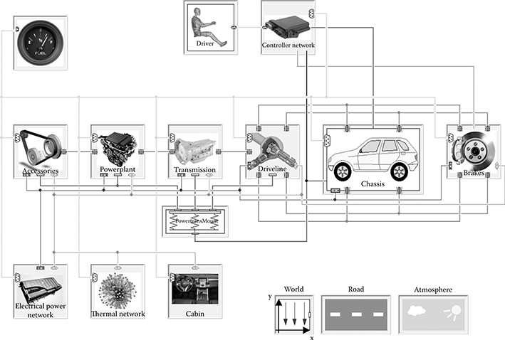
FIGURE 22.15 Vehicle model architecture. (From Batteh, J., and M. Tiller, Proceedings of the 7th International Modelica Conference, Como, Italy, pp. 823–32, Modelica Association, 2009. With permission.)
22.3.6 Real-Time Language Extensions and Interfaces
As a result of increased interest in real-time computing and model-based control system development, new language elements have been introduced in Modelica for use in embedded systems. Stemming from the ITEA2 EUROSYSLIB and ITEA2 MODELISAR projects, Modelica language extensions have been designed and included in the Modelica 3.2 Specification [1] that allow models of embedded systems to be partitioned into various elements to support model-in-the-loop, software-in-the-loop (SiL), hardware-in-the-loop (HiL) applications, rapid prototyping, [25,26] and code generation [27]. The language elements facilitate the mapping between the logical system architecture where the functional and logical behavior of the control system are specified and the technical system architecture where the concrete implementation of the logic is defined. The intent is to allow the Modelica tool to automatically translate between the logical and the technical systems given mapping information formally defined in Modelica semantics. A key feature of the implementation allows the mapping to the technical system to be defined without modification of the logical system so that a single logical model can be configured for different embedded system use cases.
The new free Modelica_EmbeddedSystems library [27] provides access to the new language elements. The library provides interfaces and examples to define the partitioning of a distributed model into tasks and subtasks, the appropriate configuration between software and hardware elements, and the communication and I/O interfaces between various elements. The configuration definition includes specifications for the various tasks, subtasks, sampling rates, target processors, device drivers, integration methods, synchronization, initialization, and so on. These features allow a model of an embedded system to integrate both model-based and hardware elements in a state-of-the-art control system development environment. In conjunction with the Modelica_EmbeddedSystems library, the new Modelica_StateGraph2 library [28] offers improved hierarchical state machines for simulation of hybrid systems and real-time applications.
A related development from the ITEA2 MODELISAR project is the development of the Functional Mockup Interface (FMI), a tool-independent standard for model exchange and cosimulation [29]. The FMI is a result of collaboration between vendors of Modelica and non-Modelica tools to facilitate model exchange between simulation tools. The goal of this effort is to gain acceptance as an open standard in the CAE community to improve model exchange between suppliers and original equipment manufacturers (OEMs). The FMI standard consists of FMI for Model Exchange and FMI for Co-Simulation. The FMI looks to be a very promising development for real-time applications, including planned support for AUTOSAR, the upcoming standard for embedded system software in vehicles.
22.3.7 Tool-Specific Features
While the focus of this work is on the Modelica language, a Modelica compiler is required to generate executable code and is thus an integral part of the real-time platform. As such, there are a number of tool-specific features that have been developed to support real-time applications. These features, in conjunction with the Modelica language, are of paramount importance and merit the following overview.
The majority of the published results for real-time simulation of Modelica models were obtained using Dymola [11]. A good discussion of the various symbolic and numerical techniques employed in Dymola to solve DAEs and generate efficient code for real-time simulation is provided in the work by Elmqvist et al. [30]. Dymola has implemented a number of advanced symbolic/numeric techniques to support real-time simulation. A key challenge for multiphysics models is the disparate time scales in a model. Resolving the fastest time scales in stiff models with explicit fixed-step integration schemes requires small step sizes, which negatively impact computational efficiency. Implicit schemes allow larger time steps but require the solution of nonlinear systems of equations. Inline integration attempts to resolve this issue by combining the discretization formulas of the integration method with the model equations [31]. The resulting set of difference equations are then subject to symbolic manipulation in an attempt to generate efficient code for real-time simulation. Mixed-mode integration involves the use of implicit schemes for fast states and explicit schemes for slow states [32]. Event handling for fixed time steps is a challenge as iteration to find zero-crossings can cause computational overruns. Thus, Dymola has implemented several techniques for event handling such as predicting the occurrence of events and step size modification to detect events and synchronize with real time following event detection. These techniques can have a drastic impact on the ability to satisfy real-time constraints for complex physical systems in Modelica [33].
A common way of addressing real-time computational constraints is the development of model variants with varying complexity and potentially varying structure. Now consider the situation where a given simulation requires a more complex model during some phases of the simulation but a reduced order model can suffice otherwise. This modeling approach results in the potential for variable structure systems with structural changes at runtime, which are difficult to handle because of the semantics of the Modelica language. A derivative language of Modelica called Sol has been developed to provide a development platform for the investigation of technical solutions for variable structure systems [34]. Sol relaxes some of the semantics of the Modelica language regarding the creation and deletion of equations at runtime to more naturally handle variable structure systems. While not a commercial tool, this impressive, open research effort includes a formal definition of the language, a parser, and even a solution platform for numerical simulation. Published results demonstrate the application of the Sol framework to a rotational mechanical system driven by an engine model [34] and on a multibody trebuchet model [35]. The work is aimed at providing guidance and suggestions for potential improvements to the Modelica language. This effort is another example of the power of an open platform to support innovation.
22.4 Application Examples
This section provides some examples of real-time applications from the Modelica literature. Since Section 22.3 mostly discussed features of the Modelica language to support real-time work, the intent of this section is to provide a flavor for selected published real-time applications of Modelica. These applications encompass many different model-based system development activities, including HiL, SiL, and controller V&V. It should be noted that many of these examples illustrate a workflow whereby the Modelica tool leverages third-party products such as MathWorks Real-Time Workshop® [36] to generate code and compile an executable for the target real-time platform.
Otter et al. [37] demonstrated a very early application of Modelica and Dymola for real-time simulation of a detailed automatic gearbox. A model for the 4-speed automatic gearbox with a planetary and Ravigneaux gear set is developed in Modelica including the torque converter and the associated clutches to enable the various gears. The gearbox model is implemented with a simple drivetrain model to create a vehicle model. The paper described in detail several of the key Modelica models, including the implementation of the clutch model. Real-time simulation was performed using the code generated by Dymola, which was compiled using Real-Time Workshop and downloaded to a dSPACE platform for simulation. This early work demonstrated real-time capability from a Modelica model using Dymola’s symbolic manipulation for DAEs.
As a demonstration of the mixed-mode integration and inline integration schemes in Dymola for real-time simulation, Schiela and Olsson [32] tested the schemes on a 6-degree-of-freedom (DOF) robot example and a vehicle drivetrain example with a diesel engine and associated air path and loads. Benchmarking was performed using standard explicit and implicit integration schemes in addition to the mixed-mode and inline schemes in Dymola. Significant reduction in computational time was reported with the newly implemented techniques.
In one of the earliest industrial applications of Modelica for real-time simulation, Toyota [33] evaluated the newly introduced capabilities in Dymola for inline and mixed-mode integration. This work was part of a larger effort to use Modelica models to support HiL controller verification efforts. The authors evaluated inline and mixed-mode integration schemes for two industry application problems that included stiff behavior. The first problem was an engine example consisting of a mean value engine model with a complete air flow path with orifice-based flow calculations including a variable geometry turbo and an exhaust gas recirculation system. The second problem was a hydraulic actuator system with valves and long pipes. The problems were simulated on different HiL platforms with the different integration schemes for benchmarking. The authors note that the advanced integration techniques result in improved real-time performance for the stiff problems including up to two orders of magnitude reduction in computational time when compared with explicit methods.
Elmqvist et al. [30,38] performed a detailed study of the modeling and real-time simulation issues associated with detailed vehicle powertrain and chassis models in Modelica. Common issues in automotive real-time simulations are described in the context of a gearbox example. The authors provide detailed information on the challenges, modeling approaches, and resulting real-time capability of a detailed automotive powertrain simulation. The authors demonstrated impressive real-time execution of a detailed vehicle dynamics model with 72 DOF on the Opal-RT platform using Dymola’s elaborate symbolic processing capabilities. Elmqvist et al. [30] provide insight into the symbolic and numerical processing capabilities of Dymola. Several different integration schemes are benchmarked and the results compared for both computational accuracy and efficiency. This work demonstrated that detailed automotive models in Modelica could be simulated in real time.
Backman and Edvall [39] illustrated the use of a real-time dynamic process simulator for a pulp paper mill to support operator training for new equipment installs. Modelica models for the paper machines and processes were developed by integration of standard models of general equipment (valves, pumps, pipes, tanks, heat exchangers, etc.) with custom models of machinery specific to the paper plant. These reusable models were integrated with the actual control system and the actual operator displays to provide a simulation-based training environment that is identical to that of the actual physical plant. The models were compiled with Dymola into a Microsoft Windows application that is used as a real-time DDE server. This training environment helps to familiarize operators with new process dynamics, displays, and interlocking logic. Furthermore, it offers a safe environment for the simulation of a wide range of scenarios and disturbances, some potentially dangerous if performed in a physical sense, that affect the process conditions. In addition to training, the models can support control strategy development and verification before hardware deployment, resulting in significant reduction in test time.
Ferretti et al. [40] developed and implemented a concept to obtain real-time simulation code directly from Modelica models in an attempt to facilitate the use of existing Modelica models in real-time applications. The implementation involved the development of a special Modelica block that is used to define the I/O variables, communication with external tasks and hardware, and execution scheduling for the simulation. This module links to the Linux RTAI operating system and is capable of creating a soft real-time binary. Testing was performed on a 7-DOF multibody model for a robotic arm. While a promising approach, the resulting model was not real-time capable, and the authors recommended model refinement to simplify the computationally intensive dynamics, particularly nonlinear low-speed friction.
Kellner et al. [41] developed techniques for the parameterization of Modelica models in HiL environments without file I/O operations. On the basis of a strong desire to separate models from parameters, The ZF Group stores model parameters in external ASCII files that are linked at initialization. This approach poses a challenge for systems such as dSPACE that do not allow file I/O operations. The authors developed a static and dynamic parameterization approach to link parameter files into the execution code. The approach was demonstrated with Dymola through a passenger car vehicle model that was simulated on a dSPACE platform.
Morawietz et al. [42] developed a Modelica model library consisting of powertrain and electrical system models in Modelica to support the development of control strategies for intelligent vehicle energy management and fuel consumption minimization. The paper describes in detail the thermodynamic model of the engine, the alternator model, and the implementation of a neural network library. A dynamic engine thermal model and associated thermal network including the oil and coolant is presented to model the impact of warm-up on engine thermodynamics and fuel consumption. A dynamic HiL environment based on dSPACE hardware was built to measure component parameters and test energy management strategies. The HiL setup allowed the interaction of the modeled engine and electrical system with alternator and battery hardware. Sample HiL results are shown for the battery voltage and various currents in the system in response to load changes.
Winkler and Gühmann [43] integrated a vehicle model in Modelica with a dynamic engine test bench to support model-based calibration of engine and transmission control units. Since the engine is represented in hardware, the vehicle model concentrates on the dynamics of the rest of the powertrain and vehicle. The Modelica models were created with Dymola and ultimately used with RT-LAB real-time software running on a standard PC. The authors also outline a detailed synchronization procedure to ensure appropriate communication interfaces and coupling between the dynamic test bench and the HiL vehicle simulation. The resulting integrated simulations allow measurement of fuel consumption and emissions from the actual engine hardware, values that are often difficult to predict analytically, over different drive cycles for a given vehicle model. The virtual vehicle model can easily be modified to represent different powertrain configurations, including both conventional and hybrid vehicles.
Ebner et al. [44] implemented an HiL solution for the development and testing of hybrid electric vehicle (HEV) components. The objective of this work is to allow testing and validation of virtual systems in conjunction with actual hardware components. The real-time system is a Suse Linux Enterprise Real-Time (SLERT) operating system. The Modelica Real-Time Interface, developed by Arsenal Research, provides the connection between Dymola for model simulation and the I/O interfaces for interaction with the hardware systems for real-time synchronization. It also permits execution of the HiL simulation directly from Dymola. Test cases for a HEV and an electric two-wheeler are presented. The HiL system included Modelica vehicle simulation models integrated with hardware battery and electrical systems as well as a dynamic test bench.
Gäfvert et al. [45] implemented a Modelica-based solution for HiL simulation of dynamic liquid food processes. Modelica models for the liquid food processes were compiled using Dymola into a real-time process simulator running on a standard Windows PC and integrated with the production control strategy. This approach results in soft-real-time capability that is sufficient for the given application. The goal of this effort was to replace costly and time-consuming predelivery hardware testing using liquid surrogates with HiL testing using the process model. HiL simulation also offers opportunities for development, testing, and V&V of the production control strategy. A dairy pasteurization process was used to evaluate the real-time HiL platform. Testing with the HiL simulations over a range of fault conditions indicated that the model-based approach discovered nearly all problems identified with the hardware testing in addition to several others that were not discovered in hardware.
Yuan and Xie [46] describe the modeling of a hydraulic steering system including the dynamic models of key components such as the priority valve and steering control unit. A Modelica model of the hydraulic steering system is then implemented in Dymola. The resulting model is used in a real-time simulation in conjunction with a vehicle model from Carsim to capture the interaction between the steering system and the vehicle dynamics through human-in-the-loop testing. Opal-RT RT-LAB is used as the real-time target. The resulting HiL setup allows various driving maneuvers to be simulated to verify the performance of the hydraulic steering system.
Blochwitz and Beutlich [47] describe various steps for creating a real-time capable model from Modelica models in SimulationX [48]. Starting from a description of the key model, compiler, and solver optimizations required for real-time simulation, the authors describe the SimulationX Code Export Wizard that guides the user through the workflow to create real-time capable models in target-independent C code. The tool can interface with targets based on Simulink® [49] and Real-Time Workshop, dSPACE, SCALE-RT, and NI Veristand. Various model reduction and analysis techniques are described to aid the modeler in the nontrivial task of model complexity reduction for computational efficiency.
Bonvini et al. [50] demonstrated the use of Modelica for HiL simulation of a robot for control design. Although the application is simplified and largely academic in nature, the work is noteworthy for the open framework that it employed. Modelica is used to create a simplified model of a robot with two rotational DOF and also for creating the control algorithm. Through the open framework documented in the paper, a HiL system is shown with an Arduino microcontroller running the control algorithm from Modelica and a PC generating the desired trajectory, simulating the Modelica model of the robot, and visualizing the 3D movement. The open framework involves the use of OpenModelica for Modelica compilation and DAE generation through XML export, Java for generating executable code, and Python for visualization. This application, while academic in terms of scope and complexity, clearly showcases the unique possibilities with the open Modelica language in conjunction with other open-source tools.
Pitchaikani et al. [51] demonstrated a closed loop real-time simulation of a vehicle with a climate control system in Modelica. The climate control system model included the air and refrigerant loops with representations for the cabin, evaporator, expansion valve, condenser, compressor, blower, heater, and air inlet door. Real-time modeling of climate control systems is a challenge because of the complex, nonlinear physical phenomena inherent in the air and refrigerant loops and computationally expensive property calculations of the two media. The vehicle model was combined with a controller model in Simulink and simulated in an Opal-RT real-time environment. Drive cycle simulations with the integrated vehicle and controller model on the HiL platform were demonstrated in real time as part of a controller verification effort.
22.5 Conclusions
Multidomain physical system modeling with Modelica has proven to be a key technology for model-based systems development. This chapter provides an overview of the Modelica language and the key features that make it a desirable modeling platform to support real-time simulation. Several different sample models are provided to provide concrete examples of the features discussed. Selected simulation results highlight the computational impact of model formulation and symbolic manipulation. Published work is reviewed to convey a sense for the variety of real-world applications from many different domains that are supported by real-time simulation with Modelica.
With continued development by the Modelica Association, enhancements to the language and standard library are ongoing. The Modelica user base continues to grow as do the tools that support the Modelica language. This growth will continue to bring cutting edge modeling and simulation technology to the forefront to support both current and future real-time model-based system development applications.
References
1. Modelica Association. 2010. Modelica: A Unified Object-Oriented Language for Physical Systems Modeling—Language Specification. Version 3.2. http://www.modelica.org/documents/ModelicaSpec32.pdf (accessed June 30, 2010).
2. Modelica Association. “Publications—Modelica Portal.” Modelica and the Modelica Association—Modelica Portal. http://www.modelica.org/publications (accessed June 30, 2010).
3. Elmqvist, H. 1978. A Structured Model Language for Large Continuous Systems. Thesis, Department of Automatic Control, Lund University, Sweden. http://www.control.lth.se/database/publications/article.pike?artkey=elm78dis (accessed June 30, 2010).
4. Cellier, F. E., H. Elmqvist, and M. Otter. 1995. “Modeling from Physical Principles.” In The Control Handbook, edited by W. S. Levine, 99–108. Boca Raton, MA: CRC Press.
5. Pantelides, C. 1988. “The Consistent Initialization of Differential-Algebraic Systems.” SIAM Journal on Scientific and Statistical Computation 9 (213): 213–31.
6. Modelica Association. “Documents—Modelica Portal.” Modelica and the Modelica Association—Modelica Portal. http://www.modelica.org/documents (accessed June 30, 2010).
7. Modelica Association. “Modelica Libraries—Modelica Portal.” Modelica and the Modelica Association—Modelica Portal. http://www.modelica.org/libraries (accessed June 30, 2010).
8. Tiller, M. 2001. Introduction to Physical Modeling with Modelica. Boston, MA: Kluwer Academic Publishers.
9. Fritzson, P. A. 2004. Principles of Object-Oriented Modeling and Simulation with Modelica 2.1. Piscataway, NJ: IEEE Press.
10. Modelica Association. “Home—Modelica Portal.” Modelica and the Modelica Association—Modelica Portal. http://www.modelica.org (accessed June 30, 2010).
11. Dassault Systemes. 2008. Dymola. Computer Software. Version 7.0. Lund, Sweden: Dassault Systemes (Dynasim AB).
12. Deltatheta. Modelica SDK. http://www.deltatheta.com/products/modelicasdk/index.jsp (accessed June 30, 2010).
13. OpenModelica. Welcome to OpenModelica. http://www.openmodelica.org/ (accessed June 30, 2010).
14. Modelon AB. JModelica.org. http://www.jmodelica.org/ (accessed June 30, 2010).
15. Nikoukhah, R. “Scicos Homepage.” Accueil—INRIA Rocquencourt. http://www-rocq.inria.fr/scicos/ (accessed June 30, 2010).
16. Cellier, F. E., and E. Kofman. 2006. Continuous System Simulation. New York: Springer.
17. Anderson, M. 1994. Object-Oriented Modeling and Simulation of Hybrid Systems. Thesis. Department of Automatic Control, Lund Institute of Technology, Sweden.
18. Tarjan, R. 1972. “Depth-First Search and Linear Graph Algorithms.” SIAM Journal of Computation 1 (2): 146–60.
19. Casella, F., M. Otter, K. Proelss, C. Richter, and H. Tummescheit. 2006. “The Modelica Fluid and Media Library for Modeling of Incompressible and Compressible Thermo-Fluid Pipe Networks.” In Proceedings of the 5th International Modelica Conference, Vienna, Austria, pp. 631–40. Modelica Association.
20. Park, R. H. 1929. “Two Reaction Theory of Synchronous Machines.” AIEE Transactions 48: 716–30.
21. Bachmann, B. 2010. “Tutorial 2: Mathematical Aspects of Modeling and Simulation with Modelica.” In Proceedings of the 6th International Modelica Conference, Bielefeld, Germany. http://www.modelica.org/events/modelica2006/Proceedings/tutorials/Tutorial2.pdf (accessed June 30, 2010).
22. Tate, E. D., M. Sasena, J. Gohl, and M. Tiller. 2008. “Model Embedded Control: A Method to Rapidly Synthesize Controllers in a Modeling Environment.” In Proceedings of the 6th International Modelica Conference, Bielefeld, Germany, pp. 493–502. Modelica Association.
23. Batteh, J., and M. Tiller. 2009. “Implementation of an Extended Vehicle Model Architecture in Modelica for Hybrid Vehicle Modeling: Development and Applications.” In Proceedings of the 7th International Modelica Conference, Como, Italy, pp. 823–32. Modelica Association.
24. Bals, J., G. Hofer, A. Pfeiffer, and C. Schallert. 2003. “Object-Oriented Inverse Modelling of Multi-Domain Aircraft Equipment Systems and Assessment with Modelica.” In Proceedings of the 3rd International Modelica Conference, Linköping, Sweden, pp. 377–84. Modelica Association.
25. Xu, X., and E. Azarnasab. 2012. “Progressive Simulation-Based Design for Networked Real-Time Embedded Systems.” In Real-Time Simulation Technologies: Principles, Methodologies, and Applications, edited by K. Popovici, P. J. Mosterman. Boca Raton, FL: CRC Press.
26. Scharpf, J., R. Hoepler, and J. Hillyard. 2012. “Real Time Simulation in the Automotive Industry.” In Real-Time Simulation Technologies: Principles, Methodologies, and Applications, edited by K. Popovici, P. J. Mosterman. Boca Raton, FL: CRC Press.
27. Elmqvist, H., M. Otter, D. Henriksson, B. Thiele, and S. E. Mattsson. 2009. “Modelica for Embedded Systems.” In Proceedings of the 7th International Modelica Conference, Como, Italy, pp. 354–63. Modelica Association.
28. Otter, M., M. Malmheden, H. Elmqvist, S. E. Mattsson, and C. Johnsson. 2009. “A New Formalism for Modeling of Reactive and Hybrid Systems.” In Proceedings of the 7th International Modelica Conference, Como, Italy, pp. 364–77. Modelica Association.
29. Blochwitz, T., M. Otter, M. Arnold, C. Bausch, C. Clauss, H. Elmqvist, A. Junghanns, et al. 2011. “The Functional Mockup Interface for Tool Independent Exchange of Simulation Models.” In Proceedings of the 7th International Modelica Conference, Dresden, Germany, pp. 823–32. Modelica Association.
30. Elmqvist, H., S. E. Mattsson, H. Olsson, J. Andreasson, M. Otter, C. Schweiger, and D. Brück. 2004. “Realtime Simulation of Detailed Vehicle and Powertrain Dynamics.” In Proceedings of the SAE 2004 World Congress & Exhibition, Detroit, MI, Paper 2004-01-0768.
31. Elmqvist, H., S. E. Mattsson, and H. Olsson. “New Methods for Hardware-in-the-Loop Simulation of Stiff Models.” In Proceedings of the 2nd International Modelica Conference, Oberpfaffenhofen, Germany, pp. 59–64. Modelica Association.
32. Schiela, A., and H. Olsson. 2000. “Mixed-Mode Integration for Real-Time Simulation.” In Modelica Workshop 2000 Proceedings, Lund, Sweden, pp. 69–75. Modelica Association.
33. Soejima, S., and T. Matsuba. 2002. “Application of Mixed Mode Integration and New Implicit Inline Integration at Toyota.” In Proceedings of the 2nd International Modelica Conference, Oberpfaffenhofen, Germany, pp. 65-1–65-6. Modelica Association.
34. Zimmer, D. 2008. “Introducing Sol: A General Methodology for Equation-Based Modeling of Variable-Structure Systems.” In Proceedings of the 6th International Modelica Conference, Bielefeld, Germany, pp. 47–56. Modelica Association.
35. Zimmer, D. 2009. “An Application of Sol on Variable-Structure Systems with Higher Index.” In Proceedings of the 7th International Modelica Conference, Como, Italy, pp. 225–32. Modelica Association.
36. MathWorks. Real-Time Workshop. http://www.mathworks.com/products/rtw (accessed June 30, 2010).
37. Otter, M., C. Schlegel, and H. Elmqvist. 1997. “Modeling and Realtime Simulation of an Automatic Gearbox Using Modelica.” In Proceedings of ESS’97 European Simulation Symposium, Passau, Germany, pp. 115–21, International Society for Computer Simulation.
38. Elmqvist, H., S. E. Mattsson, J. Andreasson, M. Otter, C. Schweiger, and D. Brück. 2003. “Real-Time Simulation of Detailed Automotive Models.” In Proceedings of the 3rd International Modelica Conference, Linköping, Sweden, pp. 29–38. Modelica Association.
39. Backman, J., and M. Edvall. 2005. “Using Modelica and Control Systems for Real-Time Simulations in the Pulp.” In Proceedings of the 4th International Modelica Conference, Hamburg, Germany, pp. 579–83. Modelica Association.
40. Ferretti, G., M. Gritti, G. Magnani, G. Rizzi, and P. Rocco. 2005. “Real-Time Simulation of Modelica Models under Linux/RTAI.” In Proceedings of the 4th International Modelica Conference, Hamburg, Germany, pp. 359–65. Modelica Association.
41. Kellner, M., M. Neumann, A. Banerjee, and P. Doshi. 2006. “Parametrization of Modelica Models on PC and Real Time Platforms.” In Proceedings of the 5th International Modelica Conference, Vienna, Austria, pp. 267–73. Modelica Association.
42. Morawietz, L., S. Risse, H. Zellbeck, H. Reuss, and T. Christ. 2005. “Modeling an Automotive Power Train and Electrical Power Supply for HiL Applications using Modelica.” In Proceedings of the 4th International Modelica Conference, Hamburg, Germany, pp. 301–07. Modelica Association.
43. Winkler, D., and C. Gühmann. 2006. “Synchronising a Modelica Real-Time Simulation Model with a Highly Dynamic Engine Test-Bench System.” In Proceedings of the 5th International Modelica Conference, Vienna, Austria, pp. 275–81. Modelica Association.
44. Ebner, A., M. Ganchev, H. Oberguggenberger, and F. Pirker. 2008. “Real-Time Modelica Simulation on a Suse Linux Enterprise Real Time PC.” In Proceedings of the 6th International Modelica Conference, Bielefeld, Germany, pp. 375–79. Modelica Association.
45. Gäfvert, M., T. Skoglund, H. Tummescheit, J. Windahl, H. Wikander, and P. Reuterswärd. 2008. “Real-Time HWIL Simulation of Liquid Food Process Lines.” In Proceedings of the 6th International Modelica Conference, Bielefeld, Germany, pp. 709–15. Modelica Association.
46. Yuan, Q., and B. Xie. 2008. “Modeling and Simulation of a Hydraulic Steering System.” SAE International Journal of Commerical Vehicles 1 (1): 488–94.
47. Blochwitz, T., and T. Beutlich. 2009. “Real-Time Simulations of Modelica-Based Models.” In Proceedings of the 7th International Modelica Conference, Como, Italy, pp. 386–92. Modelica Association.
48. ITI GmbH. SimulationX. http://www.itisim.com/simulationx_505.html (accessed June 30, 2010).
49. MathWorks. Simulink. http://www.mathworks.com/products/simulink (accessed June 30, 2010).
50. Bonvini, M., F. Donida, and A. Leva. 2009. “Modelica as a Design Tool for Hardware-in-the-Loop Simulation.” In Proceedings of the 7th International Modelica Conference, Como, Italy, pp. 378–85. Modelica Association.
51. Pitchaikani, A., K. Jebakumar, S. Venkataraman, and S. A. Sundaresan. 2009. “Real-Time Drive Cycle Simulation of Automotive Climate Control System.” In Proceedings of the 7th International Modelica Conference, Como, Italy, pp. 839–46. Modelica Association.
52. National ITS Architecture Team. 2007. Systems Engineering for Intelligent Transportation Systems. Report no. FHWA-HOP-07-069. United States Department of Transportation. http://www.ops.fhwa.dot.gov/publications/seitsguide/index.htm (accessed June 30, 2010).
53. Cellier, F. E. 1991. Continuous System Modeling. New York: Springer-Verlag.
54. Modelica Association. 2010. Modelica Tools—Modelica Portal. Modelica and the Modelica Association—Modelica Portal. http://www.modelica.org/tools (accessed June 30, 2010).