9 Modern Methodology of Electric System Design Using Rapid-Control Prototyping and Hardware-in-the-Loop
Jean Bélanger and Christian Dufour
CONTENTS
9.1 Introduction to Real-Time Simulation
9.1.2 Analysis of Simulator Bandwidth Requirements
9.1.3 Rapid Control Prototyping
9.2 Real-Time Simulator Technology
9.3 Model-Based Design Using Real-Time Simulation
9.3.2 Interaction with the Model
9.4.1 Power Generation Applications
9.4.3 All-Electric Ships and Electric Train Networks
9.4.5 Electric Drive and Motor Development and Testing
9.4.6 Mechatronics: Robotics and Industrial Automation
9.1 Introduction to Real-Time Simulation
A simulation is a representation of the operation or features of a system through the use or operation of another system [1]. For the types of digital simulation discussed in this work, it is assumed that a simulation with discrete-time and constant-step duration is performed. During discrete-time simulation, time moves forward with constant-step duration in set slices or steps of equal duration. This is commonly known as fixed time-step simulation [2]. However, it is important to note that other solving techniques that are unsuitable for real-time simulation make use of variable time steps, which helps in solving high-frequency dynamics and nonlinear systems [3]. This subject is not covered in this chapter, but it is covered in Crosbie [4].
To solve mathematical functions and equations at a given time step, each variable or system state is solved successively as a function of variables and states at the end of the preceding time slice. For the sake of clarity, we do not consider iterative solver methods that are not time-bounded. In real-time simulation, explicit or semiexplicit solvers such as State-Space Nodal [5] are preferred for the fact that their computational time at each iteration is predictable. During a discrete-time simulation, the amount of physical time, or real time, it takes to compute all equations and functions representing a system during a given time slice can be shorter or longer than the duration of the simulation time-step. Figures 9.1a and b represent these two possibilities. In Figure 9.1a, the computing time is shorter than a fixed time step (also referred to as accelerated simulation), while in Figure 9.1b, the computing time is longer. These two situations are referred to as offline simulation. In both cases, the moment at which a result becomes available is irrelevant. In fact, when performing offline simulation, typically the objective is to obtain results as fast as possible. The time that a system takes to produce a simulation depends on the computation power available and the mathematical complexity of the system model.
Conversely, during real-time simulation, the accuracy of the computations depends not only on the precise dynamic representation of the system, but also on the time duration necessary to produce results [6]. Figure 9.1c illustrates the chronological principle of a real-time simulation. For a real-time simulation to be valid, the real-time simulator that is used must accurately produce the internal variables and outputs of the simulation and do so within the same length of time that its physical counterpart would. In fact, the time required to compute the solution at a given time step must be shorter than the physical time duration of the time slice. This permits the real-time simulator to perform all operations necessary to make a real-time simulation relevant, including driving inputs and outputs (I/O) to and from externally connected devices. For a given time slice, any idle time following (or preceding) simulator operation is literally lost, as opposed to accelerated simulation, where this idle time is used to compute the equations at the next time step. In case of idle time, the real-time simulator waits until the clock ticks to the next time-step. However, if all simulator operations are not achieved within the required fixed time step, the real-time simulation is considered erroneous. Such an occurrence is commonly defined as an “overrun.”
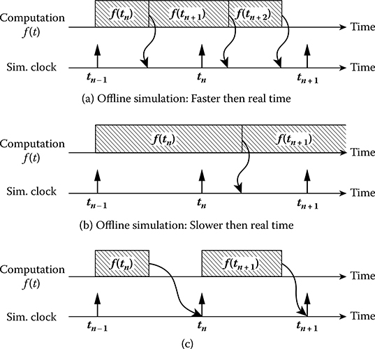
FIGURE 9.1 Real-time simulation requisites and other simulation techniques.
Based on these basic definitions, it can be concluded that a real-time simulator is performing as expected if the equations and states of the simulated system are solved sufficiently accurately, that is, within a user specification, depending on the type of phenomena that the user wants to observe, with an acceptable resemblance to its physical counterpart and without the occurrence of overruns.
9.1.1 Timing and Constraints
As previously discussed, real-time digital simulation is based on discrete time steps, where the simulator solves model equations successively. Proper step size duration must be determined to accurately represent system frequency response up to the fastest transient of interest. Simulation results can be validated when the simulator achieves real-time performance without overruns.
For each time step, the simulator executes the same series of tasks: (1) read inputs and generate outputs, (2) solve model equations, (3) exchange results with other simulation nodes, and (4) wait for the start of the next step. A simplified explanation of this routine suggests that the state(s) of any externally connected device is sampled once at the beginning of each time step of the simulation. Consequently, the state(s) of the simulated system is communicated to external devices only once per time step. If not all the timing conditions of real-time simulation are met, overruns occur and discrepancies between the simulator results and the responsive of its physical counterpart are observed.
The inherent constraint of today’s real-time simulator is the inescapable use of a discrete-time-step solver, which can become a major limitation when simulating nonlinear systems, such as a High Voltage Direct Current (HVDC) electric power system [7], FACTS [8], active filters, or drives. When nonlinear events such as transistor switching are present in a real-time simulation, because of the nature of discrete-time-step solvers, numerical instability can occur. Different solving methods have been proposed to prevent this problem [6,9], but they cannot be used during real-time simulation.
Achieving real time is one thing, but achieving it synchronously is another. With nonlinear systems, there is no guarantee that switching events will occur (or should be simulated) at a discrete-time instance. Furthermore, multiple events can occur during a single time step, and without proper handling, the simulator may only be aware of the last one. Recently, real-time simulator manufacturers have proposed solutions to timing and stability problems. Proposed solutions generally known as discrete-time compensation techniques usually involve time-stamping and interpolation algorithms [8]. State-of-the-art real-time simulators take advantage of advanced I/O cards running at a sampling rate considerably faster than fixed-step simulation [10,11]. As the I/O card acquires data faster than the simulation, it can read state changes in between simulation steps. Then, at the beginning of the next time step, the I/O card passes on to the simulator not only state information, but also timing information regarding the moment at which the state change occurred. The simulator can then compensate for the timing error.
Figure 9.2 illustrates a classic case of simulation error caused by the late firing of a thyristor in a converter circuit. In this example, a thyristor is triggered at a 90-degree angle with respect to the AC voltage source positive zero-crossing. As soon as the thyristor is triggered, current starts flowing through it. The resulting load current obtained through uncompensated real-time simulation (dotted line) is represented with some degree of error in comparison to the current flowing through the physical circuit (plain black line). This is because the event at 90 electrical degrees does not occur synchronously to the simulator fixed time step. Thus, the thyristor gate signal is only taken into account at the beginning of the next time step. This phenomenon typically induces low-frequency spurious oscillations in the simulation, for example, causing “jitter” in the motor current [12]. When jitter occurs in a discrete-time simulation, subsynchronous or uncharacteristic harmonics (amplitude variations) may be visible in the resulting waveforms. In this case, variations are evident in the thyristor current.
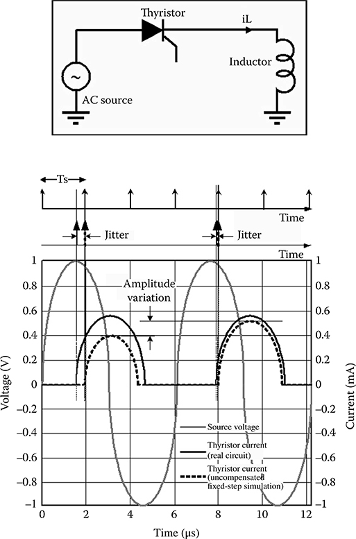
FIGURE 9.2 Timing problem in the simulation of a thyristor converter.
Finally, the use of multiple simulation tools and different step sizes during real-time simulation can cause problems. When multiple tools are integrated in the same simulation environment, a method called co-simulation, data transfer between tools can present challenges since synchronization and data validity must be maintained [13]. Furthermore, in multirate simulations, where parts of a model are simulated at different rates (with different time-step durations), result accuracy and simulation stability are also issues [14]. For example, multirate simulation may be used to simulate a thermal system with slow dynamics along with an electrical system with fast dynamics [15]. The field of multirate simulation and co-simulation environments, where multiple tools are used side by side, is still an active topic of research.
9.1.2 Analysis of Simulator Bandwidth Requirements
The criteria that will dictate the capability, size, and consequently the cost of the simulator are (1) the frequency of the highest transients to be simulated, which in turn dictates minimum step size and (2) the size of the system to simulate (i.e., the number of differential/algebraic equation to compute), which along with the step size dictates the computing power required. The number of I/O channels required to interface the simulator with physical controllers or other hardware is also critically important, affecting the total performance and cost of the simulator.
Figure 9.3 outlines the typical step size and computing power required for a variety of applications. On the left-hand side of the chart, it is observed that mechanical systems with slow dynamics will generally require a simulation time step between 1 and 10 ms, according to the rule of thumb that the simulation step size should be smaller than 5% to 10% of the smallest time constant of the system. A shorter step size may be required to maintain numerical stability in stiff systems. In addition, when friction phenomena are present, simulation step sizes as low as 100–500 μs may be required.
It is a common practice with electromagnetic transient (EMT) simulators to use a simulation time step of 30–50 μs to provide acceptable results for transients up to 2 kHz [16]. Because greater precision can be achieved with smaller step sizes, simulation of transient phenomena with frequency content up to 10 kHz typically require a simulation time step of approximately 10 μs.
Accurately simulating fast-switching power electronic devices requires the use of very small time steps to solve system equations [12]. Offline simulation is widely used in the field, but it is time consuming if no precision compromise has been made on models (i.e., by the use of average models) [17]. Power electronic converters with a higher pulse width modulation (PWM) carrier frequency in the range of 10 kHz, such as those used in low-power converters, require step sizes of less than 250 ns in duration without interpolation or 10 μs with an interpolation technique. AC circuits with higher resonance frequency and very short lines, as expected in low-voltage distribution circuits and electric rail power feeding systems, may require step sizes below 20 μs in duration. Tests that use practical system configurations and parameters are necessary to determine minimum step size and computing power required to achieve the time step chosen.
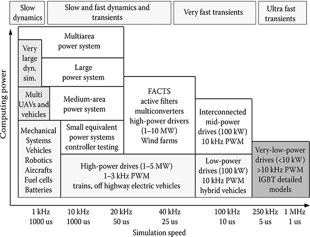
FIGURE 9.3 Simulation time step by application.
Regardless of the simulator used, both numerical solver performance and the bandwidth of interest are considerations when selecting the appropriate step size. The standard approach for selecting a suitable fixed step size for models with increasing complexity is a time-domain comparison of waveforms for repeated runs with different step sizes.
9.1.3 Rapid Control Prototyping
Real-time simulators are typically used in three different application categories [18, 19, 20 and 21], as illustrated in Figure 9.4. First, in rapid control prototyping (RCP) applications (Figure 9.4a), a plant controller is implemented using a real-time simulator and is connected to a real physical plant. RCP offers many advantages over implementing an actual controller prototype. A controller prototype developed using a real-time simulator is more flexible, less time consuming to implement, and easier to debug. The controller prototype can be tuned on the fly or completely modified with just a few mouse clicks. Also, since every internal controller state is available, an RCP can be debugged faster without having to take its cover off.
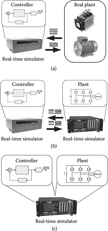
FIGURE 9.4 Application categories.
9.1.4 Hardware-in-the-Loop
For hardware-in-the-loop (HIL), the second category of applications, a physical controller is connected to a virtual plant executed on a real-time simulator, instead of to a physical plant. Figure 9.4b illustrates a small variation to HIL. In this case, an implementation of a controller using RCP is connected to a virtual plant via HIL. In addition to the advantages of RCP, HIL allows for early testing of controllers when physical test benches are not available. Moreover, virtual plants usually cost less and have parameters that have less standard deviation of the parameters due to manufacturing process or caused by environmental variations. This allows for more repeatable results and provides for testing conditions that are unavailable on real hardware, such as extreme events testing in which a real device would be damaged for example.
9.1.5 Software-in-the-Loop
Software-in-the-loop (SIL) represents the third logical step beyond the combination of RCP and HIL. With a sufficiently powerful simulator, both controller and plant can be simulated in real time on the same simulator. SIL has the advantage over RCP and HIL that no I/O are used, thereby preserving signal integrity. Also, since both the controller and plant models run on the same simulator, timing with the outside world is no longer critical. The execution time can now be slower or faster than real time with no impact on the validity of the results. SIL can, therefore, be used for a class of simulation called accelerated simulation. In accelerated mode, a simulation runs faster than real time, allowing for a large number of tests to be performed in a short period of time. For this reason, SIL is well suited for statistical testing such as Monte Carlo simulations. SIL does not have to be done in real time because no physical device is connected to the process but because Monte Carlo simulations are very time consuming, involving typically several thousand simulation runs, a real-time simulator will result in shorter completion time than offline simulation; the simulation runs slower than real time.
9.2 Real-Time Simulator Technology
Simulator technology has evolved from physical/analog simulators (e.g., HVDC simulators and transient network analyzer (TNA)) for EMT and protection and control studies, to hybrid TNA/analog/digital simulators with the capability of studying electromechanical transient behavior [22], to fully digital real-time simulators, as illustrated in Figure 9.5.
Physical simulators have served their purpose well. However, they were very large, expensive, and require highly skilled technical teams to handle the tedious jobs of setting up networks and maintaining extensive inventories of complex equipment. With the development of microprocessor and floating-point digital signal processor (DSP) technologies, physical simulators have been gradually replaced with fully digital real-time simulators.
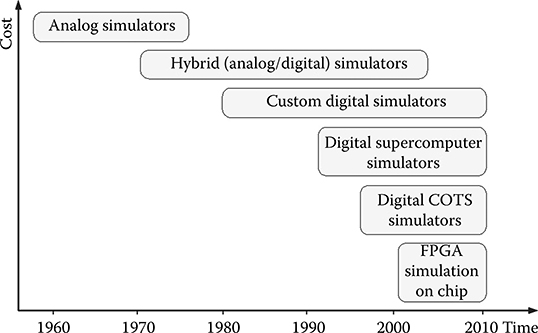
FIGURE 9.5 Evolution of real-time simulation technologies.
DSP-based real-time simulators developed using proprietary technology, and used primarily for HIL studies, were the first of the new breed of digital simulator to become commercially available [23]. However, the limitations of using proprietary hardware were quickly recognized, leading to the development of commercial supercomputer-based simulators, such as HYPERSIM™ from Hydro-Quebec [24] or RTDS™ real-time simulator [25]. Attempts have been made by a number of universities and research organizations to develop fully digital real-time simulators using low-cost standard PC technology in an effort to eliminate the high costs associated with the use of high-end supercomputers [16]. Such development was very difficult due to the lack of fast, low-cost intercomputer communication links. However, the advent of low-cost, easily obtainable multicore processors [26] (from INTEL and AMD) and related commercial-off-the-shelf (COTS) computer components has directly addressed this issue, clearing the way for the development of much lower cost and easily scalable real-time simulators. The availability of this low-cost, high-performance processor technology has also reduced the need to cluster multiple PCs to conduct complex parallel simulation. This reduces dependence on sometimes costly fast intercomputer communication technology.
COTS-based high-end real-time simulators equipped with multicore processors have been used in aerospace, robotics, automotive, and power electronic system design and testing for a number of years [27,28]. Recent advancements in multicore processor technology means that such simulators are now available for the simulation of EMT expected in large-scale power grids, microgrids, wind farms, and power systems installed in large electrical ships and aircraft. These simulators, operating under Windows, LINUX, and standard real-time operating systems, have the potential to be compatible with multi-domain tools, including simulation tools. This capability enables the analysis of interactions between electrical, power electronic, mechanical, and fluid dynamic systems.
The latest trend in real-time simulation consists of exporting simulation models to field programmable gate arrays (FPGA) [29]. This approach has many advantages. First, computation time within each time step is almost independent of the system size because of the parallel nature of FPGAs. Second, overruns cannot occur once the model is running and timing constraints are met. Last, but most importantly, the simulation step size can be very small, in the order of 250 ns. There are still limitations on model size since the number of gates is limited in FPGAs; nevertheless, this technique is promising for the future.
9.3 Model-Based Design Using Real-Time Simulation
This section explains how the model-based design methodology and real-time simulation technology are used together in the industrial development process.
9.3.1 Model-Based Design
Model-based design (MBD) is a mathematical and graphical method of addressing problems associated with the design of complex systems [30]. MBD is a methodology based on a workflow known as the “V” diagram, as illustrated in Figure 9.6 [21]. It allows multiple engineers involved in a design and modeling project to use models to communicate knowledge of the system under development in an efficient and organized manner [31]. Four basic steps are necessary in the process: (1) build the plant model, (2) analyze the plant model and synthesize a controller for it, (3) simulate the combination of plant and controller, and (4) deploy the controller.
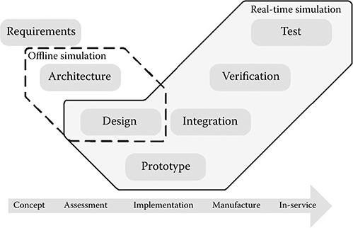
FIGURE 9.6 Model-based design workflow.
MBD offers many advantages. By using models, it provides a common design environment available to every engineer involved in creating a system from beginning to end. Indeed, the use of a common set of tools facilitates communication and data exchange. Reusing older designs is also easier since the design environment can remain homogeneous through different projects. In addition to MBD, graphical modeling tools, such as the SimPowerSystems™ for Simulink™ from MathWorks™ [32], simplify the design task by reducing the complexity of models through the use of a hierarchical approach. Modeling techniques have also been used to embed independent coded models inside the power systems simulation tool PSCAD/ EMTDC [33].
Most commercial simulation tools provide an automatic code generator that facilitates the transition from controller model to controller implementation. The added value of real-time simulation in MBD emerges from the use of an automatic code generator [34,35]. By using an automatic code generator with a real-time simulator, an RCP can be implemented from a model with minimal effort. The prototype can then be used to accelerate integration and verification testing, something that cannot be done using offline simulation. HIL testing also offers a number of interesting possibilities. The HIL process, which is the reverse of the RCP methodology, involves implementing a plant model in a real-time simulator and connecting it to a physical controller or controller prototype. By using an HIL test bench, test engineers become part of the design workflow earlier in the process, sometimes before an actual plant becomes available. For example, by using the HIL methodology, automotive test engineers can start early testing of an automobile controller before a physical test bench is available.
Combining RCP and HIL while using the MBD approach has many advantages:
Design issues can be discovered earlier in the process, enabling required trade-offs to be determined and applied, thereby reducing development costs.
Development cycle duration is reduced because of parallelization in the workflow.
Testing cost can be reduced in the medium- to long-term, since HIL test setups often cost less than the physical setups and the real-time simulator used can be typically used for multiple applications and projects.
Testing results are more repeatable since real-time simulators evidence less variability because the dynamics do not change through time the way physical systems do.
Tests that are too risky or expensive to perform using physical test benches become possible.
9.3.2 Interaction with the Model
Figure 9.7 illustrates the key advantage of real-time simulation: model interaction. These interactions can be (1) with a system user, (2) with physical equipment, or (3) with both at the same time.
It is important to note that a model executed on a real-time simulator can be modified online, which is not possible with a physical plant. Any parameter of the model can be read and updated continuously. For example, in a power plant simulation, the shaft inertia of a turbine can be modified during the simulation to determine its effect on stability, something impossible on a physical power plant. Furthermore, with a real-time simulator, all model variables are accessible during execution. As an example, in a wind turbine application, the torque imposed on the generator from the gearbox is available, since it is a modeled quantity. In a physical wind turbine, obtaining a precise torque value in real time may not be possible since the cost of a torque meter may well be prohibitive.
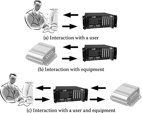
FIGURE 9.7 Types of simulator interaction.
Online model configuration and full data availability make previously unthinkable applications possible. An example of such an application is testing the ability of a controller to adapt to changes in a plant. It is, therefore, possible to verify if a controller can compensate for changes in the dynamics of the plant caused by component aging.
9.4 Application Examples
This section explains various applications of real-time simulation technology.
9.4.1 Power Generation Applications
Testing of complex electric systems shown in Figure 9.8 such as HVDC networks, static VAR compensators, static compensators, FACTS device control systems, and the integration of renewable energy sources in the grid, under steady state and transient operating conditions, is a mandatory practice during the controller development phase and before final system commissioning [30,36,37]. Testing is performed to reduce risk associated with conducting tests on physical networks. HIL testing must first be performed successfully with a prototype controller before the actual production controller is installed in the field. Thousands of systematic and random tests are typically required to test performance under normal and abnormal operating conditions [38]. This testing can also detect instabilities caused by unwanted interactions between control functions and the power system, which may include other FACTS devices that may interact with the system under test.
Protection and insulation coordination techniques for large power systems make use of statistical studies to deal with inherent random events, such as the electrical angle at which a breaker closes or the point-on-wave at which a fault appears [39]. By testing multiple fault occurrences, measured quantities can be identified, recorded, and stored in databases for later retrieval, analysis, and study. While traditional offline simulation software (e.g., ATP, EMTP) [40] can be used to conduct statistical studies during the development of protection algorithms, once a hardware relay is built, further evaluation and development may require using a real-time simulator. Typical studies include digital relay behavior evaluation in different power system operating conditions. Furthermore, relay action may influence the power system, increase distortions, and thus affect other relays. Closed-loop testing in real time is necessary for many system studies and for protection system development.
The integration of distributed generation (DG) devices, including microgrid applications and renewable energy sources (RES), such as wind farms, is one of the primary challenges facing electrical engineers in the power industry today [41,42]. It requires in-depth analysis and the contributions of many engineers from different specialized fields. With growing demand in the area, there is a need for engineering studies to be conducted on the impact that the interconnection of DG and RES will have on specific grids. The fact that RES and DG are usually connected to the grid using power electronic converters is a challenge in itself. Accurately simulating fast-switching power electronic devices requires the use of very short step sizes to solve system equations. Moreover, synchronous generators, which are typically the main generation sources on grids, have a slow response to EMT. The simulation of fast-switching power electronic devices in combination with slow electromechanical components in an electrical network is challenging for large grid benchmark studies, more so if proper computation resources are not available. Offline simulation is widely used in the field but is time consuming, particularly if no precision compromise is made on the models (e.g., use of average models for PWM inverters). By using real-time simulation, the overall stability and transient responses of the power system, before and after the integration of RES and DG, can be investigated in a timely matter. Statistical studies can be performed to determine worst-case scenarios, optimize power system planning, and mitigate the effect of the integration of these new energy sources.
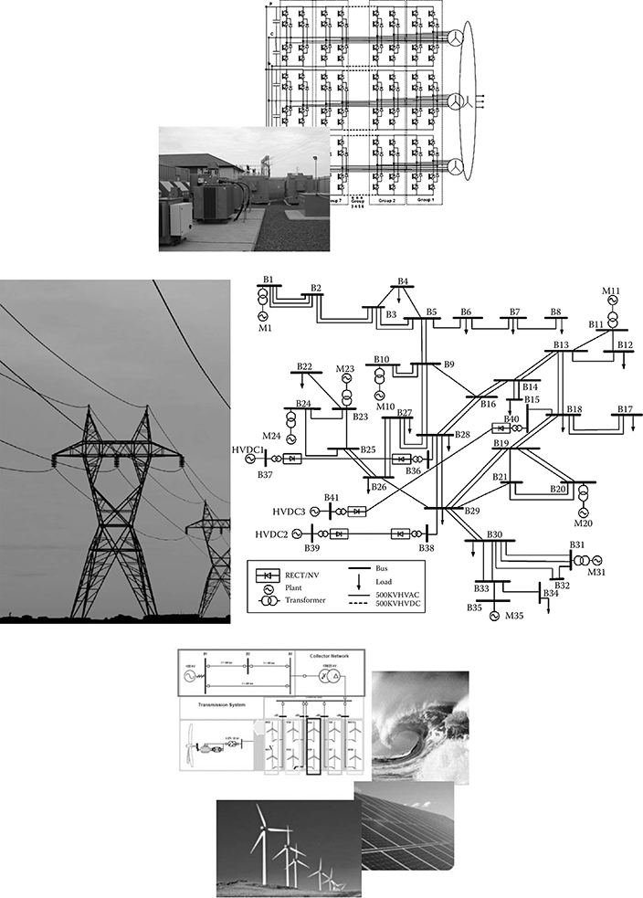
FIGURE 9.8 Power generation applications.
9.4.2 Automotive Applications
Internal combustion engine hybrid electric cars built by companies such as Toyota and Honda have become economically viable and widely available in recent years. At the same time, considerable research is underway toward the development of fuel cell hybrid electric vehicles, where the main energy source is hydrogen-based. Successful research and development of fuel cell hybrid electric vehicles requires state-of-the-art technology for design and testing. Lack of prior experience, expensive equipment, and shorter developmental cycles are forcing researchers to use MBD techniques for development of control systems [43]. For this reason, thorough testing of traction subsystems such as fuel cell hybrid vehicle is performed using HIL simulation [44], as illustrated by Figure 9.9. In this example, a real-time simulation of a realistic fuel cell hybrid electric vehicle circuit, consisting of a fuel cell, battery, DC–DC converter, and permanent magnet motor drives, with a sufficient number of I/O for real controllers in HIL mode, can now (2010) be performed with a step size duration below 10 μs [45].
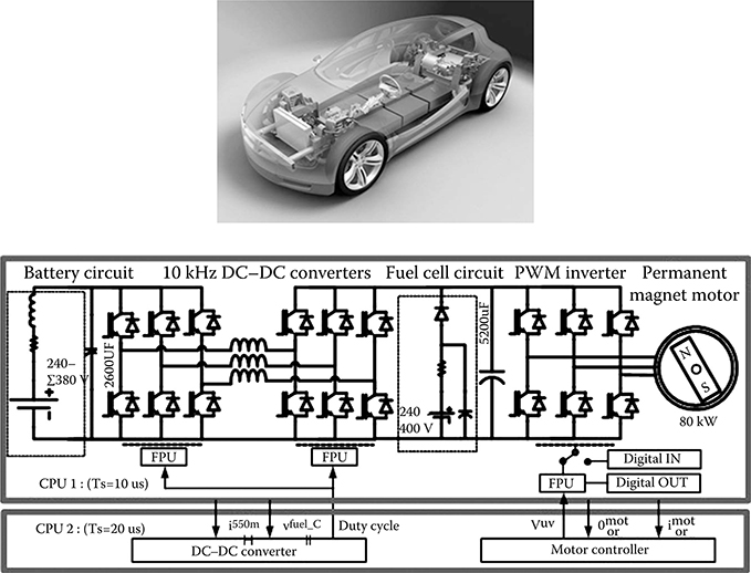
FIGURE 9.9 Automotive applications.
9.4.3 All-Electric Ships and Electric Train Networks
Today, the development and integration of controllers for electric train and all- electric ship (AES) applications is a more difficult task than ever before. Emergence of high-power switching devices has enabled the development of new solutions with improved controllability and efficiency. It has also increased the necessity for more stringent test and integration capabilities since these new topologies come with less design experience on the part of system designers. To address this issue, real-time simulation can be a very useful tool to test, validate, and integrate various subsystems of modern rail (Figure 9.10a) and marine (Figure 9.10b) vehicle devices [46]. The requirements for rail/marine vehicle test and integration reaches several levels on the control hierarchy, from low-level power electronic converters used for propulsion and auxiliary systems to high-level supervisory controls.
The modular design and redundancies built into the power system of an AES designed for combat are critical in ensuring the ship’s reliability and survivability during battle. For instance, auxiliary propulsion systems will dynamically replace the primary system in case of failure. This implies that such a power system be dynamically reconfigured, such as in zonal electric distribution systems (ZEDS) that have been recently designed for the U.S. Navy AES [47]. Therefore, power management operations must be highly efficient. Power quality issues must be kept to a minimum, and operational integrity must be as high as possible during transients caused by system reconfigurations or loss of modules.
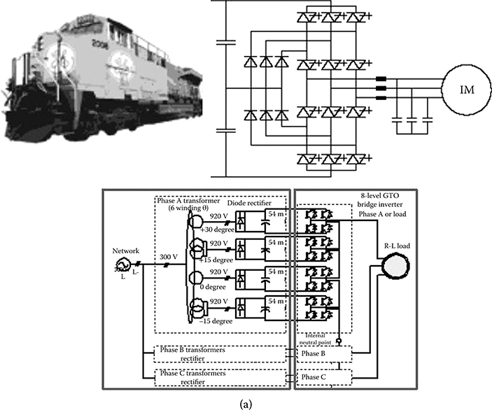
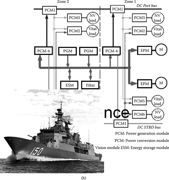
FIGURE 9.10 Train (a) and ship (b) applications.
The design and integration of an AES’s ZEDS is challenging in many ways. Such a project requires testing of the interactions between hundreds of interconnected power electronic subsystems, built by different manufacturers. Large analog test benches or the use of actual equipment during system commissioning is, therefore, required at different stages of the project. A real-time simulator can be effectively used to perform HIL integration tests to evaluate the performance of some parts of these very complex systems, thereby reducing the cost, duration, and risks related to the use of actual equipment to conduct integration tests [40].
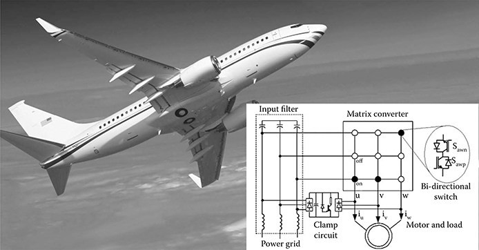
FIGURE 9.11 Aerospace applications.
9.4.4 Aerospace
Although most aerospace applications do not necessitate the extremely short step sizes required in power generation or automotive applications, repeatability and accuracy of simulation results is crucial. Safety is a critical factor in the design of aerospace systems (Figure 9.11). Accordingly, aircraft manufacturers must conform to stringent industry standards. Developed by the U.S.-based Radio Technical Commission for Aeronautics, the DO-178B standard establishes guidelines for avionics software quality and testing in real-world conditions [48]. DO-254 is a formal standard governing design of airborne electronic hardware [49].
The complex control systems found onboard today’s aircraft are also developed and tested according to these standards. As a result, aerospace engineers must rely on high-precision testing and simulation technologies that will ensure this compliance. Of course, at the same time they must also meet the market’s demands for innovative new products, built on time, according to the specifications, and within budget.
9.4.5 Electric Drive and Motor Development and Testing
A critical aspect in the deployment of motor drives lies in the detection of design defects early in the design process. Simply put, the later in the process that a problem is discovered, the higher the cost to fix it. Rapid prototyping of motor controllers is a methodology that enables the control engineer to quickly deploy control algorithms and find eventual problems. This is typically performed using RCP connected in closed loop with a physical prototype of the drive to be controlled as illustrated in Figure 9.12. This methodology implies that the physical motor drive is available at the RCP stage of the design process. Furthermore, this setup requires a second drive (such as a DC motor drive) to be connected to the motor drive under test to emulate the mechanical load. While this is a complex setup, it has proven very effective in detecting problems earlier in the design process.
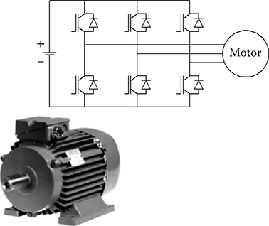
FIGURE 9.12 Smaller scale industrial and commercial applications.
In cases where a physical drive is not available or where only costly prototypes are available, an HIL-simulated motor drive can be used during the RCP development stage. In such cases, the dynamometer, physical insulated-gate bipolar transistor converter, and motor are replaced by a real-time virtual motor drive model. This approach has a number of advantages. For example, the simulated motor drive can be tested with abnormal conditions that would otherwise damage a physical motor. In addition, setup of the controlled-speed test bench is simplified since the virtual shaft speed is set by a single model signal, as opposed to using a physical bench, where a second drive would be necessary to control the shaft speed [50,51].
9.4.6 Mechatronics: Robotics and Industrial Automation
Mechatronic systems that integrate both mechanical and electronic capabilities are at the core of robotic and industrial automation applications (Figure 9.13). Such systems often integrate high-frequency drive technology and complex electrical and power electronic systems. Using real-time simulation to design and test such systems helps ensure greater efficiency of systems deployed in large-scale manufacturing and for unique, but growing applications of robotics [17].
9.4.7 Education: University Research and Development
To keep pace with the technological revolution that is underway, universities must change [52]. This transformation is necessary to create new ways to teach future engineers using a multidisciplinary approach, leveraging the possibilities offered by new tools that talented engineers are seeking, while providing them with practical experience that cultivates their creativity [53]. In this context, electronic circuit simulation programs have been in use as teaching aids for many years in electronics and control system classes. The workflow in these classes is quite straightforward: build the circuit with the circuit editor tool, run the simulation, and analyze the results. However, when it is necessary to study the effect of the variation of many parameters (e.g., oscillator frequency, duty cycle, discrete component values), this process can take a substantial amount of time [54]. In such situations, an interactive simulation based on a real-time simulator that offers the capability to change model parameters at runtime becomes a valuable teaching tool. With such a tool, changes to the model are instantly visible, providing students with the live feedback that they are looking for to acquire a feel for how a system reacts to the changes that they make to it, as illustrated in Figure 9.14.
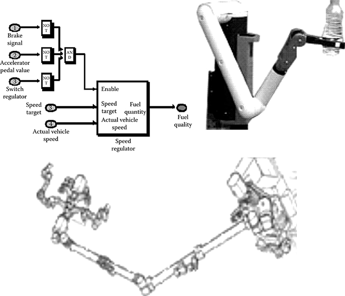
FIGURE 9.13 Mechatronic applications.
9.4.8 Emerging Applications
Real-time simulation is being used in two additional emerging applications. Since a real-time simulator can provide outputs and read inputs, it is an ideal tool for equipment commissioning and testing, as depicted in Figure 9.15a. Not only can it mimic a physical plant, it can also emulate other devices, play a recorded sequence of events, and record a device under test response. Modern simulators can also provide simulated network connections such as CAN, GPIB, and Ethernet. The application of real-time simulators to equipment commissioning and tests is common in the manufacturing of electronic control modules. For this application, the use of real-time simulators saves test bench costs and reduces testing time.
Operator and technician training is another way to put real-time simulation to good use, as illustrated in Figure 9.15b. While this application category is in an early growth stage, it offers terrific potential. For this category of application, both controller and plant are modeled in the same simulator using an SIL-like approach. The difference is that user interfaces are added to allow the operator to interact with the simulation in a user-friendly way. Interfaces such as control panels and joysticks manage user inputs, but must also provide feedback to the user about the simulation state. The advantage of using a real-time simulator for training is that the user can acquire a feeling for the controller and plant that correctly represents the real system, without the delays and limitations commonly found in training environments that are based on prerecorded scenarios.
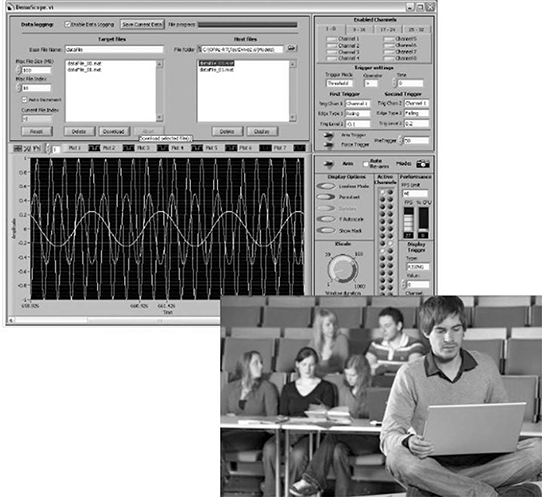
FIGURE 9.14 Education applications.
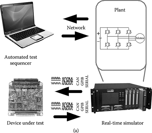
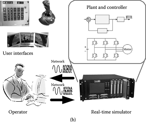
FIGURE 9.15 Emerging applications.
References
1. The American Heritage Dictionary of the English Language. 2000. Boston: Houghton Mifflin Company.
2. Dommel, H. W. 1969. “Digital Computer Solution of Electromagnetic Transients in Single- and Multiphase Networks.” IEEE Transactions on Power Apparatus and Systems, vol. PAS-88.388–99.
3. Sanchez-Gasca, J. J., R. D. Aquila, W. W. Price, and J. J. Paserba. 1995. “Variable Time-Step, Implicit Integration for Extended-Term Power System Dynamic Simulation.” In Proceedings of the Power Industry Computer Application Conference 1995, 7–12 May, pp. 183–89. Salt Lake City, UT.
4. Crosbie, R. 2012. “Real-Time Simulation Using Hybrid Models.” In Real-Time Simulation Technologies: Principles, Methodologies, and Applications, edited by Katalin Popovici, Pieter J. Mosterman. CRC Press. ISBN 9781439846650.
5. Dufour, C., J. Mahseredjian, and J. Bélanger. 2011. “A Combined State-Space Nodal Method for the Simulation of Power System Transients.” IEEE Transactions on Power Delivery 26 (2): 928–35.
6. Marti J. R. and J. Lin. 1989. “Suppression of Numerical Oscillations in the EMTP Power Systems.” IEEE Transactions on Power Systems 4: 739–47.
7. Asplung G., et al. 1997. “DC Transmission Based on Voltage Source Converters.” In CIGRE SC-14 Colloquium. Johannesburg.
8. Terwiesch, P., T. Keller, and E. Scheiben. 1999. “Rail Vehicle Control System Integration Testing Using Digital Hardware-in-the-Loop Simulation.” IEEE Transactions on Control Systems Technology 7 (3), May 1999.
9. Noda, T., K. Takenaka, and T. Inoue. 2009. “Numerical Integration by the 2-Stage Diagonally Implicit Runge–Kutta Method for Electromagnetic Transient Simulations.” IEEE Transactions on Power Delivery 24: 390–99.
10. Shu, Y., H. Li, and Q. Wu. 2008. “Expansion Application of dSPACE for HILS.” In IEEE International Symposium on Industrial Electronics, ISIE 2008, 2231–35.
11. Rabbath, C. A., M. Abdoune, and J. Belanger. 2000. “Effective Real-Time Simulations of Event-Based Systems.” In 2000: Winter Simulation Conference Proceedings, Vol. 1, 232–38. Orlando.
12. Kaddouri, A., B. Khodabakhchian, L.-A. Dessaint, R. Champagne, and L. Snider. July 1999. “A New Generation of Simulation Tools for Electric Drives and Power Electronics.” In Proceedings of the IEEE International Conference on Power Electronics and Drive Systems (PEDS ‘99), vol. 1, 348–54. Hong Kong.
13. Faruque, M. O., V. Dinavahi, M. Sloderbeck, and M. Steurer. April 2009. “Geographically Distributed Thermo-Electric Co-simulation of All-Electric Ship.” In IEEE Electric Ship Technologies Symposium (ESTS 2009), 36–43. Baltimore, MD.
14. Bednar, R. and R. E. Crosbie. 2007. “Stability of Multi-Rate Simulation Algorithms.” In Proceedings of the 2007 Summer Computer Simulation Conference, 189–94. San Diego.
15. Fang, R., W. Jiang, J. Khan, and R. Dougal. 2009. “System-Level Thermal Modeling and Co-simulation with Hybrid Power System for Future All Electric Ship.” In IEEE Electric Ship Technologies Symposium (ESTS 2009), 547–53. Baltimore, MD.
16. Hollman, J. A. and J. R. Marti. 2008. “Real Time Network Simulation with PC-Cluster.” IEEE Transactions on Power Systems 18 (2): 563–69.
17. Jin, H. 1997. “Behavior-Mode Simulation of Power Electronic Circuits.” IEEE Transactions on Power Delivery 12 (3).
18. Rath, G. 2012. “Simulation for Operator Training in Production Machinery.” In Real-Time Simulation Technologies: Principles, Methodologies, and Applications, edited by Katalin Popovici, Pieter J. Mosterman. CRC Press. ISBN 9781439846650.
19. Şahin, S., Y. İşler, and C. Guzelis. 2012. “A Real Time Simulation Platform for Controller Design, Test and Redesign.” In Real-Time Simulation Technologies: Principles, Methodologies, and Applications, edited by Katalin Popovici, Pieter J. Mosterman. CRC Press. ISBN 9781439846650.
20. Scharpf, J., R. Hoepler, and J. Hillyard. 2012. “Real Time Simulation in the Automotive Industry.” In Real-Time Simulation Technologies: Principles, Methodologies, and Applications, edited by Katalin Popovici, Pieter J. Mosterman. CRC Press. ISBN 9781439846650.
21. Batteh, J., M. M. Tiller, and D. Winkler. 2012. “Modelica as a Platform for Real-Time Simulations.” In Real-Time Simulation Technologies: Principles, Methodologies, and Applications, edited by Katalin Popovici, Pieter J. Mosterman. CRC Press. ISBN 9781439846650.
22. Su, H. T., K. W. Chan, and L. A. Snider. 2008. “Hybrid Simulation of Large Electrical Networks with Asymmetrical Fault Modeling.” International Journal of Modeling and Simulation 28 (2): 124–31.
23. Kuffel, R., J. Giesbrecht, T. Maguire, R. P. Wierckx, and P. McLaren. 1995. “RTDS: A Fully Digital Power System Simulator Operating in Real Time.” In First International Conference on Digital Power System Simulators (ICDS ‘95), April 5–7, 1995, pp. 19–24. College Station, Texas, USA.
24. Do, V. Q., J.-C. Soumagne, G. Sybille, G. Turmel, P. Giroux, G. Cloutier, and S. Poulin. 1999. “Hypersim, an Integrated Real-Time Simulator for Power Networks and Control Systems.” ICDS’99, 1–6. Vasteras, Sweden.
25. Forsyth, P. and R. Kuffel. “Utility Applications of a RTDS® Simulator.” In 2007 International Power Engineering Conference, (IPEC2007), December 3–6, 2007, 112–17. Singapore.
26. Ramanathan, R. M. Pogo Linux. http://www.pcper.com/reviews/Processors/Intel-Shows-48-core-x86-Processor-Single-chip-Cloud-Computer?aid=825.
27. Bélanger, J., V. Lapointe, C. Dufour, and L. Schoen. 2007. “eMEGAsim: An Open High-Performance Distributed Real-Time Power Grid Simulator. Architecture and Specification.” Presented at the International Conference on Power Systems (ICPS’07), December 12–4, 2007. Bangalore, India.
28. Hugh H. T. Liu. 2012. “Interactive Flight Control System Development and Validation with Real-Time Simulation.” In Real-Time Simulation Technologies: Principles, Methodologies, and Applications, edited by Katalin Popovici, Pieter J. Mosterman. CRC Press. ISBN 9781439846650.
29. Matar, M. and R. Iravani. 2010. “FPGA Implementation of the Power Electronic Converter Model for Real-Time Simulation of Electromagnetic Transients.” IEEE Transactions on Power Delivery 25 (2): 852–60.
30. Dufour, C., S. Abourida, and J. Bélanger. 2006. “InfiniBand-Based Real-Time Simulation of HVDC, STATCOM and SVC Devices with Custom-off-the-Shelf PCs and FPGAs.” In Proceedings of 2006 IEEE International Symposium on Industrial Electronics, 2025–29. Montreal, Canada.
31. Auger, D. 2008. “Programmable Hardware Systems Using Model-Based Design.” In 2008 IET and Electronics Weekly Conference on Programmable Hardware Systems, 1–12. London.
32. Sybille, G. and H. Le-Huy. 2000. “Digital Simulation of Power Systems and Power Electronics Using the MATLAB/Simulink Power System Blockset.” In IEEE Power Engineering Society Winter Meeting, 2000, Vol. 4, 2973–81. Singapore.
33. Perez, S. G. A., M. S. Sachdev, and T. S. Sidhu. 2005. “Modeling Relays for Use in Power System Protection Studies.” In the 2005 Canadian Conference on Electrical and Computer Engineering, 1–4 May 2005, 566–69. Saskatoon, SK, Canada.
34. Hanselmann, H., U. Kiffmeier, L. Koster, M. Meyer, and A. Rukgauer. 1999. “Production Quality Code Generation from Simulink Block Diagrams.” In Proceedings of the 1999 IEEE International Symposium on Computer Aided Control System Design, 1999, 213–18. Kohala Coast, Hawaii, USA.
35. Sadasiva, I., F. Flinders, and W. Oghanna. 1997. “A Graphical Based Automatic Real Time Code Generator for Power Electronic Control Applications.” In Proceedings of the IEEE International Symposium on Industrial Electronics (ISIE ‘97), Vol. 3, pp. 942–47. Guimaraes, Portugal.
36. Liu, Y., et al. 2009. “Controller Hardware-in-the-Loop Validation for a 10 MVA ETO-Based STATCOM for Wind Farm Application.” In IEEE Energy Conversion Congress and Exposition (ECCE’09), 1398–1403. San-José, CA.
37. Etxeberria-Otadui, I., V. Manzo, S. Bacha, and F. Baltes. 2002. “Generalized Average Modelling of FACTS for Real Time Simulation in ARENE.” In IEEE 28th Annual Conference of the Industrial Electronics Society (IECON 02), Vol. 2. 864–69.
38. Zander, J., I. Schieferdecker, and P. J. Mosterman, eds.2011. Model-Based Testing for Embedded Systems. Boca Raton, FL: CRC Press. ISBN 9781439818459.
39. Paquin, J. N., J. Bélanger, L. A. Snider, C. Pirolli, and W. Li. 2009. “Monte-Carlo Study on a Large-Scale Power System Model in Real-Time Using eMEGAsim.” In IEEE Energy Conversion Congress and Exposition (ECCE’09), pp. 3194–3202. San-José, CA.
40. Paquin, J. N., W. Li, J. Belanger, L. Schoen, I. Peres, C. Olariu, and H. Kohmann. 2009. “A Modern and Open Real-Time Digital Simulator of All-Electric Ships with a Multi-Platform Co-simulation Approach.” In Proceedings of the 2009 Electric Ship Technologies Symposium (ESTS 2009), April 20–22, 2009, 28–35. Baltimore, MD.
41. Paquin, J. N., J. Moyen, G. Dumur, and V. Lapointe. 2007. “Real-Time and Off-Line Simulation of a Detailed Wind Farm Model Connected to a Multi-Bus Network.” In IEEE Canada Electrical Power Conference 2007, October 25–26, 2007. Montreal, QC.
42. Paquin, J. N., C. Dufour, and J. Bélanger. 2008. “A Hardware-In-the-Loop Simulation Platform for Prototyping and Testing of Wind Generator Controllers.” In 2008 CIGRE Conference on Power Systems, October 19–21, 2008. Winnipeg, Canada.
43. Dufour, C., T. K. Das, and S. Akella. 2003. “Real Time Simulation of Proton Exchange Membrane Fuel Cell Hybrid Vehicle.” In Proceedings of 2003 Global Powertrain Congress, Ann Arbor, MI.
44. Dufour, C., T. Ishikawa, S. Abourida, and J. Belanger. 2007. “Modern Hardware-in-the-Loop Simulation Technology for Fuel Cell Hybrid Electric Vehicles.” In IEEE Vehicle Power and Propulsion Conference (VPPC 2007), September 9–12, 2007, 432–39. Arlington, TX.
45. Dufour, C., J. Bélanger, T. Ishikawa, and K. Uemura. 2005. “Advances in Real-Time Simulation of Fuel Cell Hybrid Electric Vehicles.” In Proceedings of the 21st Electric Vehicle Symposium (EVS-21), April 2–6, 2005. Monte Carlo, Monaco.
46. Dufour, C., G. Dumur, J.-N. Paquin, and J. Belanger. 2008. “A Multi-Core PC-Based Simulator for the Hardware-in-the-Loop Testing of Modern Train and Ship Traction Systems.” In the 13th Power Electronics and Motion Control Conference (EPE-PEMC 2008), September 1–3, 2008, 1475–80. Poznan, Poland.
47. Sudhoff, S.D., S. Pekarek, B. Kuhn, S. Glover, J. Sauer, and D. Delisle. 2002. “Naval Combat Survivability Testbeds for Investigation of Issues in Shipboard Power Electronics Based Power and Propulsion System.” In IEEE Power Engineering Society Summer Meeting, July 21–25, 2002, Vol. 1, 347–50. ISBN 0-7803-7518-1.
48. Radio Technical Commission for Aeronautics. 1992. “Software Considerations in Airborne Systems and Equipment Certification.” Radio Technical Commission for Aeronautics Standard DO-178B.
49. Radio Technical Commission for Aeronautics. 2000. “Design Assurance Guidance for Airborne Electronic Hardware.” Radio Technical Commission for Aeronautics Standard DO-254.
50. Bélanger, J., H. Blanchette, and C. Dufour. 2008. “Very-High Speed Control of an FPGA-Based Finite-Element-Analysis Permanent Magnet Synchronous Virtual Motor Drive System.” In IEEE 34th Annual Conference of Industrial Electronics (IECON 2008), November 10–13, 2008, 2411–16. Orlando, FL.
51. Harakawa, M., H. Yamasaki, T. Nagano, S. Abourida, C. Dufour, and J. Belanger. 2005. “Real-Time Simulation of a Complete PMSM Drive at 10 μs Time Step.” Presented at the International Power Electronics Conference, 2005 (IPEC 2005). Niigata, Japan.
52. Dufour, C., C. Andrade, and J. Bélanger. 2010. “Real-Time Simulation Technologies in Education: a Link to Modern Engineering Methods and Practices.” In Proceedings of the 11th International Conference on Engineering and Technology Education, (INTERTECH-2010), March 7–10, 2010. Ilhéus, Bahia, Brazil.
53. Min, W., S. Jin-Hua, Z. Gui-Xiu, and Y. Ohyama. 2008. “Internet-Based Teaching and Experiment System for Control Engineering Course.” IEEE Transactions on Industrial Electronics 55 (6).
54. Huselstein, J.-J., P. Enrici, and T. Martire. 2006. “Interactive Simulations of Power Electronics Converters.” In 12th International Power Electronics and Motion Control Conference (EPE-PEMC 2006), August 30–September 1, 2006, 1721–26. Portoroz, Slovenia.