
24 Systematic Derivation of Hybrid System Models for Hydraulic Systems
Jeremy Hodgson, Rick Hyde and Sanjiv Sharma
CONTENTS
24.1.1 Hydraulic Simulation Models
24.1.2 Simulating Differential Algebraic Equations
24.1.3 Parameter Abstraction of Small Masses
24.2 Network Equations for Incompressible Fluid Models
24.3 Simulation with Linear Velocity Constraints
24.3.1 Reduced Order State Vector
24.3.2 Minimum Order Momentum Equations
24.3.3 Junction Pressures and Reaction Forces
24.4 Simulation with a Singular Mass Matrix
24.4.1 Index of Differential Algebraic Equations
24.4.2 Minimum Order Dynamic Equations
24.4.3 Matrix Polynomial Equations for Algebraic States
24.4.4 Solving Systems of Polynomial Equations
24.4.5 Local Singularities in Algebraic Equations
24.5 Example: Pressure-Controlled Servo Valve
24.5.3 Mode Transition (Finite State Machine)
24.1 Introduction
Simulation models of plant or actuator dynamics are utilized throughout the development cycle of new control systems. They can be used to validate the performance of a single controller in the presence of parameter variation or to investigate the behavior when the control loop is embedded within a larger system model. The models may be for desktop analysis or as part of a real-time test harness to validate the response of hardware components to simulated inputs. Whatever the application, efficient models are required whenever large numbers of simulations are to be carried out or where there are limits on the time available to update the model at each time step. To achieve this efficiency often requires that some simplifying assumptions must be made. This chapter aims to develop a systematic approach to developing models that maintain the inherent nonlinear behavior of a hydraulic circuit but that are based on a simplified representation of fluid dynamics.
24.1.1 Hydraulic Simulation Models
Individual hydraulic component models are traditionally built up from basic foundation blocks based on the dynamics of a volume of compressible fluid and the orifice equation. More complex system models can be developed either by connecting component models directly together or by using very small volumes of fluid as interface blocks at the junctions. These interface blocks may represent actual volumes of fluid or be artificial modeling artifacts used to connect self-contained subsystem models together. The benefits of this approach are that the model can be built up in a modular fashion and that the dynamics are described in terms of systems of ordinary differential equations (ODEs), for which there are numerous robust solvers available.
It is for this reason that many commercially available hydraulic simulation packages use this approach. The disadvantage is that small volumes of compressible fluid introduce very high-frequency dynamics into the model. These high-frequency modes require small time steps to be taken and hence results in longer simulation times. The problem can be partly alleviated by the use of “stiff” solvers if real-time code is not required. If real-time code is required, then one solution is to abstract the high-frequency dynamics by assuming that these small volumes of fluid are incompressible. It is shown in Ref. [1] that making this assumption leads to a model description in terms of differential algebraic equations (DAEs), that is, the model consists of a system of unconstrained dynamic equations, along with a number of algebraic constraints that the dynamic states must satisfy.
24.1.2 Simulating Differential Algebraic Equations
Model descriptions in terms of DAEs arise in many applications, for example, in the simulation of electrical circuits, mechanical multibody dynamics, and chemical process models. An overview of current techniques used in the simulation of multi-body dynamics is given in Ref. [2], which breaks down the approaches into three categories, namely Coupled-Force Balance, Lagrange, and Kane. The Coupled-Force Balance approach assumes that each body is free to move independently, and contact between bodies is maintained by applying external forces using stiff spring damper systems. This is analogous to connecting hydraulic components by small volumes of compressible fluid. The approach suffers from generating very stiff systems of ODEs, which, as previously discussed, can be difficult to simulate.
In the Lagrange approach, it is assumed that contact is defined by a system of algebraic constraints, which are adjoined to the unconstrained dynamic equations using what are termed “undetermined,” or Lagrange, multipliers. A simplified form of the equations used to describe the dynamics of constrained rigid bodies is given in Equation 24.1, where v is the state vector of velocities, M is a positive-definite mass matrix, and F are the external forces acting on the system. The state constraints are described by the system of linear equality constraints on the velocities (W), and the Lagrange multipliers λ then represent the internal constraint forces acting at the joints.
The Lagrange approach to simulating this type of DAE is to augment the dynamic equations with the derivatives of the constraints, as shown in Equation 24.2. This results in a system of equations where the number of states equals the number of states in the original unconstrained system, plus the number of constraints. There are a number of problems with simulating this system of equations. Firstly, the initial state values must be consistent, that is, they must be chosen so that they satisfy the constraints. Secondly, because the constraints have been differentiated, any drift from the constraint manifold during simulation must be controlled. Finally, if the constraints are functions of the position states, then they must be differentiated twice before they can be augmented with the unconstrained dynamic equations. These acceleration constraints can be unstable and hence require additional stabilization to produce a stable system of equations.
The third approach to simulating multibody dynamic systems is based on the work of Kane [3], and a description of a practical simulator using this approach is given in Ref. [4]. The Kane method projects the unconstrained dynamic equations onto the constraint manifold, reducing the model to a minimal order system of ODEs, with a state vector equal in size to the number of unconstrained dynamic equations minus the number of constraints. The ability to generate a minimal order set of dynamic equations that can be simulated using standard ODE solvers makes the projection approach very appealing when simulating hydraulic models. There is one drawback, namely that a new set of minimal order ODEs must be derived whenever the number of constraints change. For example, the number of constraints will change in a hydraulic circuit model whenever a valve opens creating a new flow path or when a cylinder piston reaches its end-stop.
There are a number of approaches to handling systems with intermittent constraints. One method is to split the constraints into those that are always present and those that are likely to change. The projection approach can be used to reduce the number of equations based on the fixed number of constraints, and the remaining constraints can be implemented using the Lagrange approach as and when they become active.
This approach still suffers from the issues associated with the Lagrange approach. An alternative is to treat the system as a form of Hybrid System Model, whereby the model switches between systems of minimal order ODEs whenever the circuit topology changes. A discussion on the application of this approach to multibody system dynamics is given in Ref. [5], and an overview of a number of packages to support the simulation of this type of model is given in Ref. [6]. The decision that has to be made is whether to embed all possible sets of dynamic equations within the model before simulation or to derive new systems of equations online during the simulation. As the intent is to derive models that can run as efficiently as possible, a system by which all models are implemented before simulation is demonstrated in this chapter.
24.1.3 Parameter Abstraction of Small Masses
The mass matrix M is always assumed to be of full rank when using the constraint embedding techniques described in Refs. [1,4]. This means that the mass matrix of the reduced order equations will also have full rank and hence be invertible during the simulation. To fully specify the dynamics of a hydraulic circuit may require that some very small masses are introduced to act as connecting elements between larger objects, and these small masses can introduce high-frequency dynamics, leading to slow simulations, and potential instabilities. This chapter extends the work by Pfeiffer and Borchsenius [1] by introducing an approach that can simulate the resulting minimum order dynamic equations when the mass matrix is singular due to making these small masses to zero.
24.1.4 Structure of Chapter
The remainder of the chapter is organized as follows. In Section 24.2, the DAEs are derived that describe the dynamics of a hydraulic system when the fluid in the pipes, cylinders, or orifices is assumed to be incompressible. The approach by which these DAEs are reduced to a minimal order system of ODEs is then outlined in Section 24.3. In Section 24.4, the method of simulating the minimal order ODEs when the mass matrix is singular is described. The approach is demonstrated in Section 24.5 using, as an example, a circuit consisting of a servo valve controlling the fluid pressure in a closed pipe. Finally, conclusions are presented in Section 24.6.
24.2 Network Equations for Incompressible Fluid Models
The basis for a simulation model of connected hydraulic components containing incompressible fluid is a system of unconstrained momentum equations and a system of linear algebraic constraints. The unconstrained momentum equations are given in Equation 24.3, where v is the vector of fluid velocities augmented with states describing the motion of mechanical components such as cylinder pistons and valve spools. M is a diagonal matrix of fluid and component masses, and F(v) is the known forcing function given in Equation 24.4. For the type of hydraulic system under consideration, the forcing function consists of terms representing the external pressure sources at the interfaces to the system (PI), velocity-dependent friction terms (WV v), and the pressure drop across open orifices (∆PO). The pressure drop across an orifice is assumed to obey the orifice equation in Equation 24.5. In this case, flow through an orifice is assumed to be turbulent, and the fluid density (ρ) is independent of pressure and temperature. This does not discount extending the equations to include changes in flow regime as described in Ref. [7], by making ρ and Cd functions of the current state values.
In addition to the known forcing functions, there are unknown internal constraint forces as illustrated in Figure 24.1. The constraint forces consist of pressure forces acting at fluid junctions (PJ), reaction forces between components in contact with their end-stops (FR), and the pressure drop across closed orifices (∆PC).
The unknown constraint forces are related to a system of algebraic constraints. The velocity constraints include the requirement that the sum of the flows into a junction must be zero (WJ), that flow through closed orifices (WC) must be zero, and that the motion of components that have reached their end-stops (WR) must be zero. The combined system of constraints can then be represented by W in Equation 24.6.
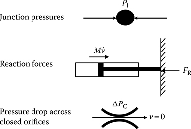
FIGURE 24.1 Internal constraint forces acting in hydraulic system models.
24.3 Simulation with Linear Velocity Constraints
The aim in this section is to derive a minimal order system of ODEs, which satisfies the unconstrained dynamics in Equation 24.3, subject to the system of linear constraints on the velocities in Equation 24.6. The basis for the derivation is that a system of n dynamic equations subject to m constraints can be reduced to a system of equations with v = n − m independent states.
24.3.1 Reduced Order State Vector
The relationship between the full state vector (v) and the reduced set of independent states () is through the transformation matrix α in Equation 24.7.
The transformation matrix α is not unique but has to be determined so that the full state vector will always satisfy the constraint equations. This can be achieved if the columns of α form the basis vectors of the null space of the constraint equations. If α satisfies that requirement, then the inner matrix product in Equation 24.8 will be satisfied for all values of the independent states.
One method for deriving α is given in Ref. [8]. In this case, the independent states are selected to be a subset of the full state vector as shown in Equation 24.9.
If the constraint matrix is partitioned as in Equation 24.10, then can be defined in terms of , and α is given by Equation 24.11.
This approach works well provided the selection of the independent states leads to a tractable system of linear equations (i.e., W2 is invertible). Making a suitable selection is not always straightforward either when there are a large number of states or when there are a large number of models to be analyzed. An alternative approach described in Ref. [9] uses the singular value decomposition (SVD) of the constraint matrix to derive the basis vectors of the null space at each time step during the simulation. This provides a robust and numerically stable approach, but can be computationally expensive and leads to the integration of states that are not directly related to the physical states of the system.
The approach taken is to determine which states can be selected as independent states before creating the simulation model. There are functions available in MathWorks Symbolic Math Toolbox™ [10] to derive the null space of the constraint matrix symbolically, and as the form of the resulting matrix is the same as in Equation 24.7, the independent states can be determined by a simple inspection of the rows of the matrix for a single entry of a unit gain. Within the simulation model, the null space matrix is regenerated using the indices of the selected states to be integrated and the formulation in Equation 24.11. The main benefit of doing this is that only a minimal amount of information must be stored with the model to define the independent state vector for each mode.
24.3.2 Minimum Order Momentum Equations
The minimum order dynamic equations can be derived once the relationship between the full and the reduced order state vectors has been established. The time derivative of the full state vector is related to the reduced state vector by Equation 24.12.
Substituting Equation 24.12 into the unconstrained dynamic equations in Equations 24.3 and projecting the equations onto the constraint manifold by multiplying through by αT leads to a minimum order system of ODEs that have the form given by Equation 24.13. The forcing function in Equation 24.13 is given by Equation 24.14, and the mass matrix is given by Equation 24.15.
24.3.3 Junction Pressures and Reaction Forces
The reduction procedure described in Section 24.3.2 creates a system of ODEs that can be simulated using standard solvers. In the process, the constraint forces have been lost from the model description. The first stage to regenerate these forces is to derive an expression for the rate of change of the dependent states as a function of the independent states. If the constraint matrix is partitioned in Equation 24.10, then after differentiation, it can be rearranged to give the expression for in Equation 24.16.
The dynamic equations in Equation 24.3 can also be partitioned as shown in Equation 24.17. The unknown internal forces can be regenerated by substituting Equation 24.16 into Equation 24.17 and rearranging to give Equation 24.18.
24.4 Simulation with a Singular Mass Matrix
In Section 24.3, the mass matrix of the unconstrained dynamic equations must have full rank if the mass matrix of the reduced order equations () is to be inverted during simulation. If some of the very small masses of fluid are made equal to zero to remove the high-frequency dynamics that they introduce, then this assumption will no longer hold. If is singular, then the dynamic equations in Equation 24.13 are said to be quasi-linear DAEs, and an extensive description of the techniques available to solve this type of system is given in Ref. [11]. Sections 24.4.1 to 24.4.5 describe the method of determining the index of the resulting DAEs when the mass matrix is singular and also a method of simulating the equations.
24.4.1 Index of Differential Algebraic Equations
The index of the DAEs is found by extracting the “hidden” algebraic constraints from the original equations. The algebraic constraints G0 are determined by projecting the dynamic equations in Equation 24.13 onto the null space of the mass matrix using the projection β that satisfies Equation 24.19. The resulting constraint equations in Equation 24.20 define the manifold on which the states can travel.
The dynamics of the constrained system is then found by augmenting the original equations with motion at a local tangent to the constraint manifold, as shown in Equation 24.21. If the augmented mass matrix has full column rank, then the system has index 1. If the mass matrix does not have full column rank, then the above procedure is repeated. That is, the hidden constraints of the augmented system are determined and a new system of equations is derived by augmenting the dynamic equations with the derivative of the new constraints. The index of the DAEs is defined by the number of times the procedure must be repeated before the augmented mass matrix has full column rank.
The hydraulics models in Equation 24.13 have index 1, and it is feasible to simulate the system of overdetermined equations in Equation 24.21 directly. The problem is that the number of independent states is defined by the size of the state vector minus the number of hidden algebraic constraints. The initial values of the full state vector must therefore be consistent (i.e., lie on the constraint manifold), and any drift from the constraint manifold during the simulation must be controlled. The approach discussed in Ref. [11] overcomes these issues by selecting a minimum number of independent integrated states from the state vector. The integrated states can then be used to determine algebraically the remaining states so that the hidden constraints are satisfied. This is similar to the method described in Section 24.3, but now, the constraints are defined by nonlinear functions of the states, and they are implicit within the model description.
24.4.2 Minimum order Dynamic Equations
A minimal order system of dynamic equations can be derived by partitioning the state vector in Equation 24.22 into independent states that are integrated in time and algebraic states that are derived at each time step from a function of the integrated states. The reordering of the integrated and algebraic states into the full state vector is achieved through the permutation matrix Π. The selection of which independent states are chosen from the full state vector is the same as in Section 24.3, namely by inspection of the symbolically derived null-space matrix β.
The rate of change of the algebraic states is derived by differentiating the constraint equations in Equation 24.20 to give Equation 24.23, where the time dependency of the orifice areas in the constraint equations is accounted for by the third term in
Rearranging Equation 24.23 into Equation 24.24, and substituting into the original equations in Equation 24.13, produces the minimum order dynamic equations in Equation 24.25, where the columns of P form the the basis vectors of the range space of the mass matrix. These equations represent a minimal order system of ODEs that satisfy G0 and where the resulting mass matrix is invertible. The problem is now to determine the relationship between the integrated and algebraic states when the constraint equations are nonlinear in nature.
24.4.3 Matrix Polynomial Equations for Algebraic States
This section describes the derivation of the relationship between the integrated and the algebraic states in the reduced order model. On the basis of the original formulation of the forcing function in Equation 24.5, the algebraic constraints can be expressed in Equation 24.26 in terms of the partitioning of the state vector in Equation 24.7. The matrix representing the pressure drop across open orifices (WO) is partitioned in Equation 24.27, and the dependent states () are related to the independent states () by Equation 24.28. The notation v |v| in Equation 24.26 defines the signed square value of each element in the state vector.
The constraints in Equation 24.26 can be rearranged in Equation 24.29 for the unknowns , where the matrices A, B, C, D are given by Equations 24.30 through 24.33.
24.4.4 Solving Systems of Polynomial Equations
There are a number of ways to solve the system of polynomial equations in Equation 24.29 for the unknown states. The approach chosen is the iterative Newton (or Newton–Raphson) method given in Equation 24.34, where the Jacobian of the constraint matrix is given by Equation 24.35. This approach has proven to be robust, and standard ODE solvers can still be utilized as the iterative procedure is only invoked when the solver requires the derivatives of the independent integrated states. The iterative procedure is still considered an acceptable approach if the equations are to be implemented in a real-time simulation code, as the maximum number of iterations can be limited to guarantee that the solution will be found in the available time.
Rather than inverting the Jacobian matrix, the velocity states are updated at each iteration by solving the system of linear equations in Equation 24.36 for the increment in the velocity estimates ∆v.
The equations in Equation 24.36 are solved using the QR decomposition of the Jacobian matrix in Equation 24.37, where Q is orthogonal, R is upper triangular, and E is a permutation matrix determined so that the values on the leading diagonal of R are in decreasing order. The QR decomposition is determined during the simulation using the FORTRAN DGEQP3 function provided in the work by Anderson et al. [12] and described in the work by Quintana-Ort et al. [13]. The efficiency of these routines compared to other implementations is outlined in the work by Foster and Liu [14].
Substituting the matrix QR decomposition into Equation 24.36 and multiplying through by QT leads to Equation 24.38. This equation can easily be solved for ∆z as R is upper triangular. The calculated solution is reordered into the desired vector of increments using the permutation matrix in Equation 24.39.
An additional benefit of decomposing the Jacobian in this way is that it provides an estimate for the rank of the matrix. The diagonal elements of R provide an approximation to the singular values, and any singular value near zero indicates that the matrix is rank deficient. If that is the case, then a minimum norm solution can be derived using the more accurate SVD described in Section 24.4.5.
24.4.5 Local Singularities in Algebraic Equations
Under certain conditions, the Jacobian of the constraint equations may be locally singular. This can occur when the orifice areas become very small just before, or after, a transition between modes. In this case, a modified Newton’s method is used (see Ref. [15]), where the aim is to determine the minimum norm solution to the equations, that is, the solution where the state vector has the smallest magnitude. The method uses a generalized outer inverse of the Jacobian to update the state vector. The outer inverse is determined using the more robust SVD of the Jacobian. The form of the decomposition is given in Equation 24.40, where U and V are orthogonal matrices, Σ is a diagonal matrix containing the singular values, and the rank of the Jacobian (r) is given by the number of nonzero diagonal elements in Σ.
An outer inverse (denoted by #) of the Jacobian is defined as any matrix where the relationship in Equation 24.43 is satisfied. On the basis of the SVD, an outer inverse can be shown to be given by Equation 24.44, and the modified Newton method is then given by Equation 24.45. The SVD is calculated during the simulation using the FORTRAN DGESVD function in Ref. [12], and although it is computationally more expensive to calculate compared to the QR decomposition described previously, the fact that it is only required at a few points during the simulation means that it does not adversely affect the efficiency of the simulation approach.
24.5 Example: Pressure-Controlled Servo Valve
24.5.1 Model Definition
This section demonstrates the derivation and implementation in the MathWorks Simulink® [16] product of a hybrid-system model for the hydraulic circuit shown in Figure 24.2. The circuit consists of a two-stage servo valve controlling the pressure in a 6 m long hydraulic pipe that is terminated at one end. The first stage in the servo valve consists of a flapper mechanism driven by a torque motor. The second stage spool is acted upon by a pilot pressure from the first stage as well as a spring force to center the spool when not under load. In addition, there is a small internal volume of fluid within the valve that acts on the spool and provides a feedback mechanism to control the pressure at the output port. A more detailed description of the operation and use of the servo valve is provided in Ref. [17].
The signal flow diagram in Figure 24.3 shows the fluid flow into the four internal junctions (circles) due to either flow through connecting orifices (solid lines) or the motion of the spool itself (dashed lines). The aim is to simulate the dynamics of the servo valve when the fluid within these small connecting volumes is assumed to be incompressible.
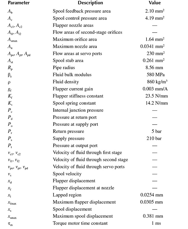
Table 24.1 provides a description of each of the parameters within the model, along with representative numerical values. The level of detail within this model is typical of an initial system-level definition before more detailed performance models are developed.
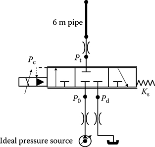
FIGURE 24.2 Circuit schematic for pressure-controlled servo valve.
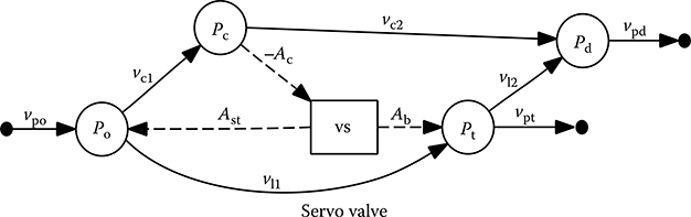
FIGURE 24.3 Signal flow diagram for pressure-controlled servo valve.
TABLE 24.1
Description Of Servo Valve Parameters
24.5.2 Model Dynamics
Some parts of the model are represented by systems of ODEs that are simulated using standard solvers. The response of the flapper (xd) in Figure 24.4 to a change in input current (iy) to the torque motor is assumed to be first order with a time constant equal to τm. The transfer function is given in Equation 24.46, where gf provides the steady-state gain between the current input and the achieved flapper displacement.
The displacement of the flapper xf at the nozzle is then given in Equation 24.47, where Kf is the flapper spring constant, An is the null position area, and Xfb is a bias. he resulting flapper nozzle areas are given by Equation 24.48.
Although the fluid within the servo is treated as incompressible, the fluid within the connected pipe is treated as compressible as the volume of fluid is significantly greater than that within the servo valve. The compressibility also provides an important memory of the fluid pressure when the valve is centered, and the pipe is effectively isolated from the rest of the system. For this example, the fluid pressure P within the pipe is determined from Equation 24.49, where βe is the effective bulk modulus, Vp is the volume of fluid within the pipe, and the flow rate Qt is determined in Equation 24.50. Treating the fluid in this case as a single lumped volume is a simplistic representation used to demonstrate the methodology. More detailed transmission line dynamic models described in Ref. [17] could equally have been used to investigate pressure peaking and oscillations following step inputs from the valve.
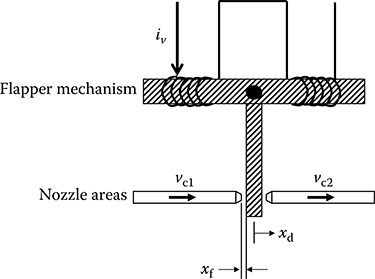
FIGURE 24.4 First-stage flapper displacement and nozzle area.
24.5.3 Mode Transition (Finite State Machine)
The discrete modes of operation must be established before the model dynamics can be derived. The modes can be defined by the relationship between the orifice areas and the position of the flapper or spool. The fluid flows through the second stage of the valve at speeds vl1 and vl2, and the respective orifice areas Al1 and Al2 are functions of the spool position shown in Figure 24.5. The figure shows that there are five discrete modes depending on whether the spool has reached its end stops (in which case vs = 0), or whether the orifices are fully closed in which case either vl1 = 0 or vl2 = 0. The flapper mechanism provides three additional modes depending on whether the flapper blocks one of the nozzle areas. In total, there are 15 discrete modes, and each has its own defined set of minimal order dynamic equations.
Control over switching between sets of dynamic equations is governed by the finite state machine implemented using the MathWorks Stateflow® product [18] and shown in Figure 24.6. The flapper and the spool are controlled through two independent parallel states. The transition between modes is governed by events triggered by a zero-crossing signal in the model. Events can occur because of either an orifice opening or closing or contact between a physical object and its end-stop. In the case of contact occurring, the subsequent release of the object is triggered by a change in sign of the calculated reaction force.
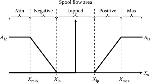
FIGURE 24.5 Second-stage orifice areas versus spool position.
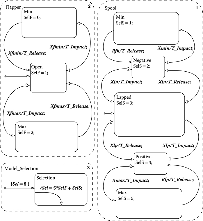
FIGURE 24.6 Finite state machine for pressure-controlled servo valve.
The very nature of the finite state machine representation means that it is ideal for including additional features that are of interest to the control engineer. In particular, the effect on the system behavior of introducing faults into the system is easily investigated by introducing trigger signals that force the model to transition into a failure state. An example where this would be appropriate is the case where a valve becomes stuck open or closed and cannot move until the failure is cleared.
24.5.4 Dae Equations (“Positive” Mode)
This section defines the system of DAEs when the spool is in the Positive mode where the orifice between the return line and the outlet port (Al2) is fully closed. The full velocity state vector and the internal junction pressures are defined in Equation 24.51. Two mass cases are considered for comparison. The first assumes that that there is a small mass of fluid in each line and in the second case all the mass elements are assumed to be negligible and are set to zero. If there is a zero mass matrix, then the dynamics of the flow through the servo valve reduces to a system of algebraic equations that must be solved at each time step for the reduced order state vector.
The flow constraints at the junctions are defined by the matrix WJ given in Equation 24.52. These constraints are maintained for all modes of operation and can be considered to be configuration constraints. The additional constraint (WC) introduced because of the closed orifice Al2 is given in Equation 24.53.
In this mode, there are eight velocity states and five linear constraints. This leads to a minimum order system consisting of three independent states. The selection of the independent states from the full state vector is made by direct inspection of the symbolically derived basis vectors for the null space of the constraint matrix. The derived symbolic matrix is shown in Equation 24.54, with the rows and columns rearranged so that the order of the states is consistent with that in Equation 24.11.
24.5.5 Simulation Results
The simulated responses to a series of step changes in demanded output pressure are shown in Figures 24.7 and 24.8. Each figure shows the simulation results from the following four model implementations:
An incompressible fluid model with a full mass matrix
An incompressible fluid model with all masses within the servo made equal to zero
A purely compressible fluid model, simulated using a “stiff” solver
An incompressible fluid model with a zero mass matrix running in discrete time (updated at 1000 Hz)
Figure 24.7 shows for each of the above models the pressure at the internal junction within the servo valve and the controlled pressure at the output port. Figure 24.8 shows the spool position and the resulting flow into the pipe. The dynamic response of each model implementation is very close, demonstrating that little accuracy has been lost by making the assumption that small volumes of fluid within the servo valve act instantaneously.
The transition between systems of reduced order dynamic equations is demonstrated in Figure 24.9, which shows the spool position and the identification number for the model that is being executed. The plot demonstrates that all five modes relating to the second-stage spool have been entered during the simulation.
A comparison of the average time taken to run each of the Simulink models is shown in Table 24.2. The models were simulated using MathWorks MATLAB® version R2006b, running on a PC with an Intel® Dual Core2 CPU running at 2.13 GHz. Model (1) clearly takes the longest time to simulate, demonstrating the detrimental effect of introducing small masses of fluid to act as connecting elements. By comparison, the simulation time of Model (3) is significantly faster, demonstrating that current “stiff” solvers are very efficient. Simulating this model using the default variable step solver (ODE45) proved to be prohibitively slow by comparison. The simulation time of Model (2) is less than half that of Model (3), which demonstrates the proposed aim of this work, namely that being able to take larger time steps during the simulation because of the removal of the high-frequency modes outweighs the additional computational overhead to implement a DAE solver. The greatest improvement in runtime is achieved with Model (4) where all the continuous time integrators were replaced with discrete time states, and the very fast dynamics of the torque motor were replaced by a constant gain.
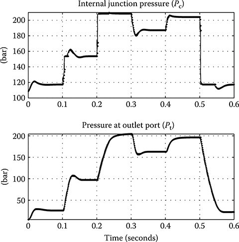
FIGURE 24.7 Simulated junction pressures: incompressible with a full mass matrix (solid line); incompressible with a singular mass matrix (dashdot line); compressible (dashed line); incompressible with a singular mass matrix and discrete time (dotted line).
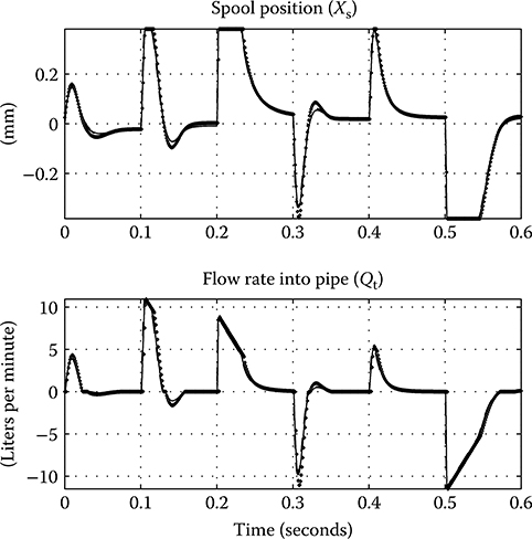
FIGURE 24.8 Simulated servo valve spool position and resulting flow rate into pipe.
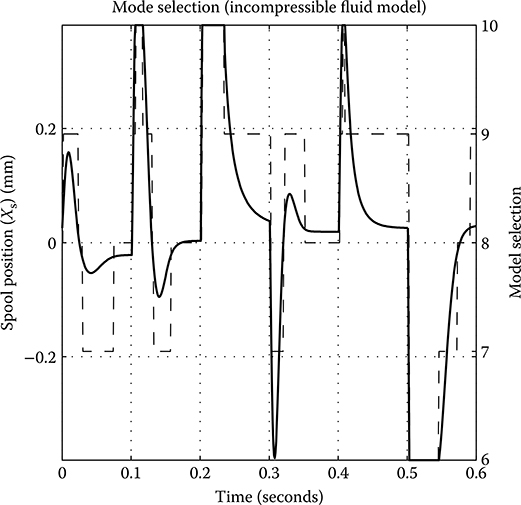
FIGURE 24.9 Simulated switching behavior of the spool position (solid line) and the corresponding model selection (dashed line).
TABLE 24.2
Average Simulink Runtime (Simulated Time = 0.6 S)
Model |
Fluid Type |
Mass Matrix |
Solver |
Time (S) |
1 |
Incompressible |
Full |
ODE45 |
37.76 |
2 |
Incompressible |
Singular |
ODE45 |
0.79 |
3 |
Compressible |
— |
ODE23tb |
1.90 |
4 |
Incompressible |
Singular |
Discrete |
0.31 |
24.6 Conclusions
This chapter has demonstrated a systematic approach to deriving hybrid system models of a hydraulic circuit using a combination of symbolic and numeric techniques. The models are defined in terms of the original circuit layout, but the dynamics of small volumes of fluid are abstracted to instantaneous changes in state. The efficiency of the resulting models, using standard off-the-shelf solvers, has been tested by comparing simulation times with models that use small volumes of compressible fluid as connecting elements and current state-of-the-art “stiff” solvers. The simulation times of the hybrid system models have been shown to be lower than the reference models using a “stiff” solver. The greatest improvement in simulation time is achieved when the hybrid system models are run in discrete time, which is not an option when relying on the “stiff” solvers. The ability to run models in discrete time faster than real time demonstrates the potential to run simulations of hydraulic circuits in true real time, while still maintaining a faithful representation of the inherent nonlinear behavior of the circuit.
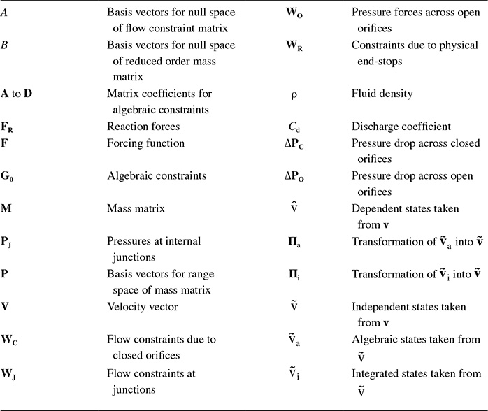
24.7 Symbol List
Acknowledgment
The authors wish to thank Airbus Operations Ltd for their support during this research.
References
1. Pfeiffer, F., and F. Borchsenius. 2004. “New Hydraulic System Modelling.” Journal of Vibration and Control 10(10): 1493–515.
2. Gillespie, R. B., and J. E. Colgate. 1997. “A Survey of Multibody Dynamics for Virtual Environments.” In Proceedings of the ASME International Mechanical Engineering Conference and Exposition, Dallas, Texas, Vol. 61, pp. 45–54.
3. Kane, T. R. 1961. “Dynamics of Nonholonomic Systems.” Journal of Applied Mechanics 28: 574–78.
4. Gillespie, R. Brent. 2003. “Kane’s Equations for Haptic Display of Multibody Systems.” The Electronic Journal of Haptics Research 3: 1–20.
5. Gillespie, R. Brent., V. Patoglu, I. I. Hussein, and E. R. Westervelt. 2005. “On-Line Symbolic Constraint Embedding for Simulation of Hybrid Dynamical Systems.” Multibody System Dynamics 14(3–4): 387–417.
6. Mosterman, P. J. 1999. “An Overview of Hybrid Simulation Phenomena and Their Support by Simulation Packages.” In Hybrid Systems: Computation and Control: Second International Workshop. Berlin/Heidelberg: Springer.
7. Merritt, H. E. 1967. Hydraulic Control Systems. 2nd ed. New York: John Wiley & Sons, Inc.
8. Wampler, C., K. Buffington, and J. Shu-hui. 1985. “Formulation of Equations of Motion for Systems Subject to Constraints.” Journal of Applied Mechanics 52: 465–70.
9. Singh, R. P., and P. W. Likens. 1985. “Singular Value Decomposition for Constrained Dynamical Systems.” Journal of Applied Mechanics 52: 943–48.
10. The MathWorks, Inc. 2006. Symbolic Math Toolbox User’s Guide. 3.1.5 ed. Natick, MA: The MathWorks, Inc.
11. Rabier, P. J., and W. C. Rheinboldt. 2001. “Theoretical and Numerical Analysis of Differential-Algebraic Equations.” Handbook of Numerical Analysis 8: 183–542.
12. Anderson, E., Z. Bai, C. Bischof, J. Demmel, J. Dongarra, J. Du Croz, A. Greenbaum, S. Hammarling, A. Mckenney, and D. Sorensen. 1990. “Lapack: A Portable Linear Algebra Library for High-Performance Computers.” Technical Report CS-90-105, University of Tennessee, Knoxville, TN.
13. Quintana-Ort, G., X. Sun, and C. Bischof. 1998. A BLAS-3 Version of the QR Factorization with Column Pivoting. SIAM Journal on Scientific Computing 19(5): 1486–94.
14. Foster, L. V., and X. Liu. In press. “Comparison of Rank Revealing Algorithms Applied to Matrices with Well Defined Numerical Ranks.” SIAM Journal on Matrix Analysis and Applications, unpublished manuscript. http://www.math.sjsu.edu/~foster/rank/rank_revealing_s.pdf.
15. Nashed, M. Z., and X. Chen. 1993. “Convergence of Newton-Like Methods for Singular Operator Equations Using Outer Inverses.” Numerische Mathematik 66: 235–57.
16. The MathWorks, Inc. 2006. Simulink Reference. 6.5 ed. Natick, MA: The MathWorks Inc.
17. Tunay, I., E. Y. Rodin, and A. A. Beck. 2001. “Modeling and Robust Control Design for Aircraft Brake Hydraulics.” IEEE Transactions on Control Systems Technology 9: 319–29.
18. The MathWorks, Inc. 2006. Stateflow and Stateflow Coder Reference. 6.5 ed. Natick, MA: The MathWorks Inc.