
20 Automotive Real-Time Simulatio: Modeling and Applications
Johannes Scharpf, Robert Höpler and Jeffrey Hillyard
CONTENTS
20.2 RT Techniques for Automotive Systems
20.3 Achieving RT in Engine Simulation
20.3.1 Choosing the Right Type of Model
20.3.3 Model Verification and Validation
20.3.4 From the Model to a RT Executable
20.4 RT Implementations in the Automotive Industry
20.4.1 Diagnosing a Faulty EGR Valve
20.1 Introduction
The automotive industry is continuously demanding shorter development cycles in order to maintain competitiveness. For this reason, car manufacturers have always been adopting state-of-the-art strategies to shorten the time to market such as simultaneous engineering, rapid product development, and front loading of the development process. These are examples where simulation techniques are key enablers. The use of simulation in the development process leads to an early increase of knowledge. Consequently, subsequent processes can start sooner, which amounts to time and cost savings. Nowadays, simulation is used throughout all phases of product development, in the conceptual design and requirements phase, during design of hardware and software, and in computer-aided production planning. However, it still is most efficient in early stages of the development process. Particularly, the modeling and simulation of dynamic systems accelerates development in early phases, for example, in feasibility studies by evaluating the potential of new topologies using virtual prototypes or in the automated and model-based design of control strategies. Simulation allows technical prototypes to mature quicker and at the same time reduce their number. Moreover, fewer experiments on test stands are necessary.
The behavior of technical systems can be described and investigated by dynamic system modeling and simulation. Real-time (RT) techniques serve as a natural supplement to modeling and simulation and allow for the running simulation to “connect” with real-world systems in various ways. Hardware-in-the-loop (HIL) methods are an explicit incarnation of this coupling of virtual and technical systems in that one or more virtual components of the simulation model are replaced with physical ones. The physical parts of the technical system interact with the numerical model that simulates the realistic physical behavior of the remaining virtual components as sketched in Figure 20.1.
The HIL system has two main requirements that must be met: Firstly, the interface has to provide real physical entities such as force, torque, current, etc. This is done by actuators, sensors, and their controls. If the system to be interfaced is a computer such as an embedded system, coupling is somewhat simpler because it takes place at an electrical signal level. This method is beneficial especially for the development and testing of electronic control units of computer-based systems, for example, engine control units (ECUs) in Schuette and Ploeger (2007). Secondly, physical behavior of the simulation model must execute synchronously with the physical system parts, or in real time. A closer look reveals that it is sufficient to have the relevant physical information, or states, from the simulation available only at every point in time when virtual and physical parts, which may also be human operators, must interact through the interface.
This chapter presents some aspects of how automotive development benefits from RT and HIL methods. Section 20.2 provides an overview of challenges and restrictions of modeling automotive systems in a RT context. Simulating multidomain systems such as passenger cars requires special care when choosing modeling approaches, approximations, and mathematical formalisms. Section 20.3 focuses on the RT simulation and control of a combustion engine—itself a classic multidomain system—as a prime example. Section 20.4 highlights several applications of the RT methods and models but also addresses the limitations of these approaches. Finally, Section 20.5 presents some concluding thoughts.
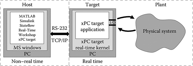
FIGURE 20.1 Example of a HIL system layout (From Mosterman, P. J. et al., Handbook of Networked and Embedded Control Systems, edited by Dimitrios Hristu-Varsakelis and William S. Levine, 419–46, Birkhäuser, Boston, 2005. With permission.)
20.2 RT Techniques for Automotive Systems
Numerical RT simulation of the behavior of any dynamic system is based on specific formulations of the dynamics. These models are mathematical relationships represented either as differential equations, difference equations, or hybrid approaches (Mosterman and Biswas 2002). Particularly, the modeling of automotive systems imposes several challenges:
A vehicle comprises a plurality of physical domains.
The time scales of the dynamics cover several orders of magnitude.
A combinatorial variety of vehicle types and configurations exists.
A vital need for disclosure of intellectual property by the original equipment manufacturers (OEM) is evident.
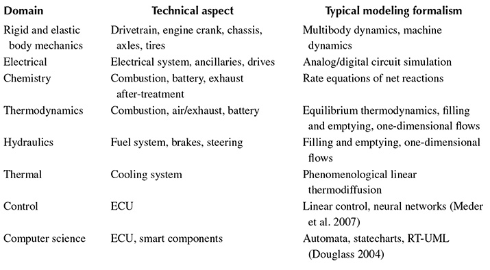
Although today’s vehicles rely increasingly on computers, they are still classical multidomain systems. Table 20.1 lists the predominant domains involved and common ways to model these domains in the field of RT simulation.
According to the continuous nature of almost all technical parts, their physics is described by partial differential equations (PDEs) and hence numerically best through the finite element method (FEM) and related methods. As shown in Table 20.1, this abstraction of physical reality is not often considered in the field of automotive RT simulation. With this in mind, which abstractions are considered and for what reasons?
Many types of formalisms, such as FEM or computational fluid dynamics (CFD) with their fine-grained discretization in space and time, can be ruled out for RT applications. Complex models that must observe an immense number of variables over an extended period of time, such as those for simulating gas flow, challenge current computing hardware. If that is the case, then how can one accelerate the computational ability of a technical system model? Computational demand is proportional to the number of simulation state variables x(t). Reducing to a lower number of simulation state variables is beneficial for two reasons: First, the smaller system can be formulated by ordinary nonlinear differential equations (ODEs) or differential algebraic equations (DAE), where
TABLE 20.1
Modeling Domains In Automotive Rt Simulation
governs the time evolution of x(t) (Vidyasagar 1993). The variable u represents the control inputs, and the variable p represents all parameters that do not appear as time derivatives. This approach often delivers satisfying quality of simulation results. The vast amount of simulation variables present in an FEM formulation is condensed to several physically meaningful states and allows for control laws to be designed much easier. The restrictions of this process are obvious: one must be careful when fundamental assumptions for the reduced model will not hold or when interesting phenomena will be completely neglected. In the field of internal combustion engine (ICE) simulation, these are certainly regions where one approaches the limits of thermodynamic equilibrium. The most prominent ones are the near-supersonic processes that take place in a turbocharger or the processes of combustion and gas exchange in a cylinder.
Secondly, an often overseen issue is that the reduction to a few simulation states affects the necessity for obtaining suitable data. Efforts to parameterize the model may reduce considerably because the governing differential equations take lumped values. For instance, a total mass is required instead of a mass distribution, or a scalar value or characteristic map of a heat transfer coefficient is used instead of a thermodiffusion process. Particularly in the automotive field, a valid and consistent set of data leading to parameters p for the parameterization of simulation models is difficult to obtain. Intellectual property issues are one reason for this. The main reason, however, lies in the early, or conceptual, phase of technical design where employing simulation tools is most advantageous: necessary data at this point in time are either scarce, unconsolidated, or simply not available for use in the simulation. This situation is aggravated by the fact that good data are essential for reliable simulation results. The reader is referred to Section 20.3.2 for more details.
Apart from the mathematical formulation of the causal behavior of an automotive system, there is a second distinctly important aspect to RT modeling and simulation: the notion of time. The most obvious way in which the treatment of time affects RT simulation is through the time discretization within the numerical simulation. Numerical integration schemes make time discrete by using fixed or variable step sizes and project the approximation of the exact ODE/DAE solution onto a sampling grid (Brenan et al. 1987). This grid must satisfy several requirements in order to lead to a meaningful solution:
The computational load induced by the evaluation of the simulation model at each grid point must match the computing power of the RT platform to avoid task overruns. Depending on the type of RT system, such task overruns either can be tolerable or must be avoided at all costs (Schuette and Ploeger 2007). Automotive applications such as vehicle dynamics test rigs traditionally use sampling rates of 1 kHz. This restricts the integration scheme to being a fixed-step method where the number of grid points is proportional to computational load. The Forward Euler method (Brenan et al. 1987) is the most prominent among them in that it guarantees a finite execution time.
The eigenfrequencies of the model impose an upper boundary on the used step size. Especially for engine applications, this leads to sampling rates of at least 100 kHz as mentioned in Section 20.3.1 for calculating the in-cylinder pressure.
Automotive systems often contain highly reactive subsystems. As a consequence, it is, for example, for a HIL application, not sufficient (although necessary) to have the simulation run in synchrony with a physical process. Synchronicity with the physical process is superseded by the more stringent requirement of reactivity. Well-defined reaction times to external stimulation are crucial in embedded ECU applications. Particularly, the reaction of the cylinder and combustion model to the timing-critical fuel injection signals must take place within a time frame of tens of microseconds (see Section 20.4.2).
Amenability to RT execution is also affected by the way time itself is modeled, which tends to be less obvious as it is more implicitly incorporated in the modeling formalism. The states in a continuous-time model, for example, formulated as an ODE/DAE system, may change smoothly over time. In contrast with this type of model, there are discrete-event models where the state is an element belonging to a discrete set and will change abruptly over time, which is well suited to efficiently model abstract-switching behavior. This discontinuous behavior is often modeled as a finite-state machine, statecharts, or a state-transition diagram. In RT applications where computational efficiency is paramount, RT simulation models are usually combinations of continuous and discrete behavior, also known as hybrid dynamic systems. Although well-suited to RT applications, these introduce additional complexity in terms of numerics and modeling; see Mosterman and Biswas (2002) for more details.
There is a large variety of tools for RT modeling and simulation. Some approaches provide the possibility to model any hybrid dynamic system, without restrictions to the physical domain, in a modular and block-oriented way. Prominent examples are native Simulink® (Simulink 2004) and Modelica (Modelica 2010). While the first employs causal modeling, the latter is an acausal modeling formalism, which has certain advantages, for example, for model inversion. Multidomain tools with a special focus on automotive systems are, for example, ASCET-MD (ASCET-MD 2009), for the development of embedded automotive control systems, GT-Suite (GT-Suite 2009), and AMESim (AMESim 2009) for zero and one-dimensional modeling of physical systems with an option to generate RT capable code.
20.3 Achieving RT in Engine Simulation
This section shows the tasks and challenges in practical RT modeling of automotive systems. Like a passenger vehicle, the combustion engine is a complex multiphysics system in its own right. Without neglecting generality, this section focuses on the modeling of combustion engines, particularly their crucial intake/exhaust gas and fuel subsystems.
20.3.1 Choosing the Right Type of Model
There are a considerable number of approaches to modeling combustion engines, but just a few are amenable to RT applications. A physical formulation of the dynamics will be stressed because of its superior properties in terms of its ability
To extrapolate into regions where no measurements are available
To reuse models and parameters
To reduce the effort required for parameterization
To immediately understand the modeled phenomena
In this section, black-box approaches such as neural networks or model order reduction are considered a complement to PDE- or ODE-based methods (Meder et al. 2007). The number of domains involved is considerable, leading to a heterogeneous physical description and rich dynamics of the complete system. That is why most resulting models are either restricted to being a single domain model or a hybrid of both black-box and physical formulation, often resulting in gray-box models.
Among the most complicated, and also most interesting, dynamics in an automotive system may be the gas-exchange phenomena during a working cycle in the cylinder and the intake air and exhaust paths. Turbulent flows of multiphase media within complex geometries, heat transfer, and intricate chemical reactions, for example, during combustion, call for CFD models because of their resolution capabilities in time and space (Chung 2003). These models, however, are still far from being RT capable on standard hardware, for example, FIRE (AVL FIRE 2006), mainly because of the discretization in two or three dimensions. Classical methods of order reduction or the usage of neural networks with a focus on control theory are sometimes applied to reduce complexity. Papadimitriou, for example, shows a method to transform complex one-dimensional flow models into an RT neural network model of a combustion engine (Papadimitriou et al. 2005).
A more physical way of reducing the complexity of PDE solutions is the use of modal and lumped formulations of the dynamics in which symmetries are exploited or assumed. The engine cycle calculation (ECC) partitions gas volumes into ideally mixed finite volumes and ends up with a set of coupled ODEs that are solved while satisfying the conservation laws, as shown in Merker et al. (2006). The technical analogy is a set of plenums or coolers coupled by nozzles. The very complex and nonequilibrium aspects such as heat release rate and heat transfer are augmented as parametric or semiphysical models (see, e.g., Vibe [1970]) that allow for the adaptation of the model to varying operating points. An investigation of the eigenfrequencies of these models reveals that typical sampling rates must lie in the order of magnitude of 100 kHz to obtain realistic results for, for example, the in-cylinder pressure of a high-rev gasoline engine. Especially, the heat transfer to the cylinder walls, the piston, and the cylinder head is treated usually by empirical models as this process is much too complex to model from first principles. A more realistic modeling of a direct injection combustion process or the formation of engine emissions can be approximated within the ECC. The cylinder volume then has to be partitioned into two to several hundred coupled zones (Heywood 1989). The ECC is a powerful method offering a wide range of application. Common applications are development of control strategies, sensitivity analysis, combustion process development, and ECU testing. The computational complexity is at the limits of current processor power providing cause to the emergence of commercial RT models (DYNA4Engine 2009; ASM InCylinder 2006).
Mean value engine models (MVEMs) are a classical way of modeling the processes inside the combustion engine. Similar to ECC, these are based on a DAE/ ODE formulation, but the physical states are considered within a more macroscopic time scale. States are considered mean values with respect to a time range of three to five engine revolutions (Jensen et al. 1991). This is sufficient to model fast changing processes such as the opening of the exhaust gas recirculation (EGR) valve. Desired states are engine speed, engine torque, and manifold pressure to name just a few. In terms of complexity and computational effort, they rank below the ECC (Hendricks and Sorenson 1990). For the description of engine phenomena that are too complex for modeling the physics from first principles, dependent and independent variables are separated to be able to employ simple empirical models or mapped data from measurements (Jensen et al. 1991). The strength of MVEMs lies in their ability to be easily adapted to other engines. Their compact mathematical formulation requires only a comparably small number of parameters and can be calibrated to a particular engine with a small set of measurements (Hendricks and Sorenson 1990). MVEMs are often utilized in the development of control strategies and in model-based diagnostics. See Section 20.4 for some HIL applications.
State-free approaches such as engine torque maps represent a simple way to model engine behavior. These are very popular, especially in ECU applications, because they are computationally robust and efficient while offering fairly high accuracy if using data obtained by (often relatively few) engine measurements. On the other hand, maps are almost ruled out for modeling transient behavior accurately (Gheorghiu 1996), and they can potentially introduce undesired nonlinearities into the dynamics of a controlled system.
In the end, the purpose of RT engine simulation is to deliver a system’s response with respect to time that is physically correct and free of contradictions. Therefore, the choice of an appropriate model for a specific investigation or task is an intricate trade-off between available computing power, required sample rates and response times, and validity of the modeled dynamics. Figure 20.2 relates the computational complexity to time scales of characteristic phenomena in engine modeling. The gray area depicts the region of applications currently possible on standard processing hardware.
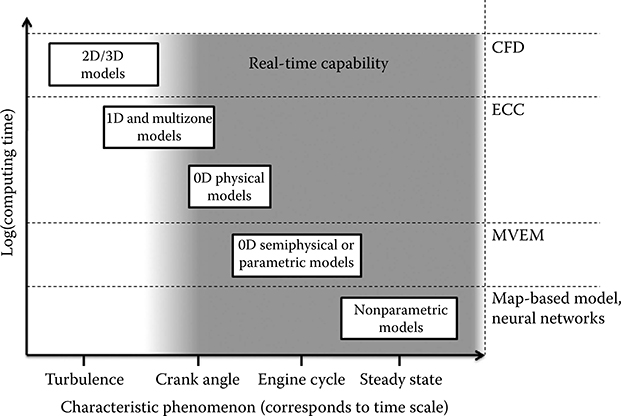
FIGURE 20.2 Relationship between engine model complexity and modeled phenomena.
20.3.2 Data Preparation
As pointed out in Section 20.2, a model of the dynamics of a technical system is composed of (1) a description of the physical behavior, (2) model parameters p, and (3) initial conditions. In order for a model to be able to sufficiently replace the physical component of a system, it is imperative that the data used are sufficiently precise and correct. Insufficient care while preparing model data or modeling will almost certainly lead to erroneous simulation results. Furthermore, data preparation takes a significant amount of time as part of the process of modeling and simulation. For these reasons, the steps of data preparation as well as model verification and validation are investigated in more depth here.
Data is almost never directly suitable to be used “as is” with the simulation model. Because of this, data preparation, sometimes known as preprocessing, is necessary to extract and transform raw data into a form suitable for the model. Data preparation is, in essence, a model of the parameters for the simulation model. For RT models, two practicalities stand out. Firstly, any calculation that can be done prior to simulating decreases the computational load. Secondly, the data must be adapted regarding structure and type to suit the model, if only because RT models often approximate complicated physical relationships, as shown in Section 20.3.1, by using lookup tables.
Data preparation requires prior knowledge of the simulation model to know which data are required as both data and model are intimately linked. Designing the data preparation process can take up a substantial amount of time and end up being an iterative process. Data preparation can roughly be divided into (1) data extraction and (2) data transformation for our purposes here. The process is schematically depicted in Figure 20.3.
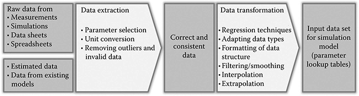
FIGURE 20.3 Flow diagram of data preparation steps.
The sources of data are manifold. They could be measurements, simulation results, data sheets, or spread sheets provided from a supplier. For the case that not all input data is available, missing data must be estimated until the remaining data are provided. This may be sufficient to get the model up and running and to even start with testing. The following three steps will lead to correct and consistent data regarding units and values:
Parameter selection is the process of identifying the correct parameters necessary to parameterize the model. There may often be many more parameters measured or provided (e.g., in a data sheet) than is necessary.
Often the provided data is not specific in terms of physical units, coordinate systems, and measurement conditions. A typical problem that arises in engine applications is the absence of reference conditions for a table of turbocharger operating points, which renders the data practically unusable (Moraal and Kolmanovsky 1999). Some modeling languages such as Modelica or Simscape™ have variable classifications that support using correct units or even the type of variable such as force or mass.
Removing outliers and invalid data will be necessary as soon as measurements are intended to be used as model inputs or for the extraction of model parameters. Problems during experiments can be sensor failures or incorrect settings that can lead to invalid data.
Data transformation will process the data according to the model requirements regarding quality, type, and structure of the input data. Data quality refers to the smoothness of data and the availability of data as a usable format. Filtering and smoothing remove discontinuities in the input data. This can help prevent the simulation of models based on such data from aborting and increases computational efficiency even for cases where a simulation could run but must take small time steps over a discontinuity to satisfy tolerances. Because data were measured at scattered points, it is often necessary to carry out interpolation to map the values onto an equidistant grid. Extrapolation will extend input data to cover regions that lie beyond the range of the measurements. Regression techniques (Izenman 2008; Ljung 1999) are used to identify model input parameters from measured data. The type of parameter depends on the number of input variables and can be, for example, scalars or n-dimensional lookup tables. Finally, all input data must conform to the requirements of the simulation model with respect to file format, memory specifications, and similar formal matters. It is a part of the data transformation process to ensure such requirements are fulfilled.
An automated process can be very valuable for data preparation because, if implemented, the user is rewarded with a reliable, time-saving, and convenient method of creating the input data set necessary for the simulation model. This is especially advantageous when the input data have been modified or improved. Directly after data preparation, it is helpful to visualize the results. Simply visualizing data in the form of plots is not only a way of identifying errors in the data, it is also a way of understanding the simulation model and its implementation. One beneficial side effect of preparing data is revealed when the user of the simulation model also carries out the data preparation but was not involved in the modeling: The user is then forced to view the data that indicate how the model was implemented. In this manner, the user becomes more aware of the model while working with the data.
20.3.3 Model Verification and Validation
Along with building a simulation model and preparing data to be used in the model, the process of verifying and validating (V&V) the simulation model is an essential step in striving toward accurate and reliable simulation results. Performing V&V is important for all types of simulation models but even more so for RT simulation applications where coupling to real-world subsystems requires quantitative correctness of the model behavior.
Model verification can be defined as ensuring that the computer program of the computerized model and its implementation are correct (Sargent 2007). This could be the transformation of a flowchart or a mathematical model consisting of equations into a computer program that can be executed. Model validation may be defined as substantiation that a computerized model within its domain of applicability possesses a satisfactory range of accuracy consistent with the intended application of the model (Schlesinger et al. 1979). The relationships between the computerized model, the conceptual model, and the technical system that is being modeled (the “real system”) are illustrated as the Sargent Circle shown in Figure 20.4. The cross- dependencies stand out in the sense that the entire process of V&V is iterative. Finding a mistake late in the model validation phase may even require reevaluating the conceptual model and modifying it. Such a change can have an extensive influence on the model behavior, leading to an entirely new testing process that must be started from the very beginning. This can have far-reaching consequences as there may be other models or components being designed that depend on having an accurate model and the design of which now must be postponed. It is for this reason that modeling errors should be caught as soon as possible.
There are many principles that should be accounted for to ensure successful V&V. Some of the most prominent ones are
The simulation model is only valid for the tested conditions.
A valid model does not imply credible and accurate results.
Successful subsystem testing does not guarantee model credibility in its entirety.
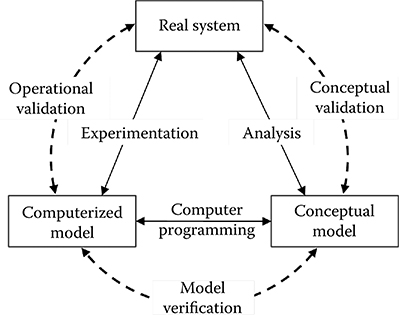
FIGURE 20.4 Simplistic overview of the process of model verification and validation. (From Sargent, R. G., Proceedings of the 2007 Winter Simulation Conference, Washington, DC, 2007. With permission.)
Carrying out V&V requires extensive testing for dynamic system models. One general method of doing this is presented by Lehmann (2003). Different types of tests are examined in Sargent (2007), for example:
Compare simulation results to real measured values from the technical system.
Compare simulation results to results from other valid models with at least comparable complexity.
Test extreme inputs or initial conditions.
Obtain expert opinion on the input–output relationship of model.
Perform steady-state and transient testing.
As suggested above, there can never be 100% validity. Ideally, the best chances for success derive from testing thoroughly and often by starting at the function level, continuing up through the subsystem and component level, and finally ending at the top system level. Each simulation model is unique, though, and so benefits from customized and detailed testing procedures. Moreover, testing thoroughly and efficiently is further complicated because the model implementation blends complex behavior on mathematical, numerical, and execution levels as described in the following section.
20.3.4 From the Model to a RT Executable
Simulation in this context mainly denotes numerical time integration. Given the model of a dynamic system 0 = f(x, x, ẋ, u, p, t) with parameters p, control inputs u, and the initial states x(t = tstart), one can solve the initial-value problem by means of numerical integration schemes. As pointed out in Section 20.2, under RT conditions one is mostly restricted to using schemes with a guaranteed execution time
and, therefore, mainly to explicit and fixed-step-size methods. Unfortunately, these methods in particular provide limited accuracy and stability when solving stiff, discontinuous, or constrained systems that often arise in the field of engineering (Eich-Soellner and Führer 1998). In order to reconcile accuracy and efficiency, integration schemes can be carefully chosen for each domain and RT model or submodel. For example, higher order single-step methods, or approximations of implicit methods where iterative solutions are truncated (Eich-Soellner and Führer 1998), can be implemented in order to meet RT requirements. Some high-performance RT solutions are even able to switch the equations and integration schemes depending on the current engine model state (DYNA4Engine 2009).
Code generation is the final step influencing the performance of an executable RT simulator. Though tedious, some dynamics model descriptions, controller, and integration schemes are still implemented by manual coding, for example, for reasons of limited resources in embedded systems. However, nowadays this approach is restricted to specific automotive applications and very expensive because of the combinatorial complexity in terms of vehicle types and configurations. When using modeling formalisms such as Simulink, the high-level, possibly graphical, model description can be automatically transferred to C code or binaries for a specific RT platform or embedded system. Prevalent tools are Real-Time Workshop® or TargetLink for generating code from Simulink models. Dymola (2009) compiles textual or graphical models in Modelica. Exploiting a symbolic representation of the model offers interesting options to automatically enhance computational performance. Mixed-mode integration, and particularly the method of inline- integration (Elmqvist et al. 1995), leads to potentially large but computationally efficient code, especially attractive in RT applications.
20.4 RT Implementations in the Automotive Industry
RT methods couple virtual and physical technical subsystems. The goal is to test physical and virtual components under practical conditions without requiring the complete system. Actual target hardware ECUs are tested using signals generated from an engine simulation on HIL test stands. Earlier stages in a model-based design process might rely on more virtual configurations: in the software-in-the-loop (SIL) configuration generated code of a control unit model is connected with a plant model. The system might neglect, for example, sensor effects and does not even run in RT. The same holds for processor-in-the-loop (PIL), but in this case, controller code runs on the target platform (Mosterman et al. 2004). Methods like HIL are attractive options in model-based development of control schemes for dynamic systems. Within the automotive industry these methods are not restricted to controller design and parameterization but are also applied (1) to quality assurance and approval of functions for testing the reaction to short circuits, cable failure, electromagnetic compatibility, and fail-safe behavior, (2) to compatibility within the control unit network in terms of interfaces and communication, and (3) to the testing of diagnostic functions (Schuette and Ploeger 2007).
There are a number of advantages of HIL methods in the field of combustion engines:
Reproducibility: A simulation environment eliminates unwanted influences, such as those resulting from varying ambient pressure or temperature, and there is no limit to the amount of testing since there is no wear on virtual components.
Cost effectiveness: Fuel and preconditioning of media are not necessary, which leads to less energy consumption and therefore significantly reduced operating costs.
Development time: HIL component testing allows for fewer engine test bed or roller test bench experiments.
Automation: Tests can be run in an automated fashion, without requiring human interaction, which enables many configurations to be used simply by loading a different engine model.
Safety: Testing extreme modes of operation does not carry the risk of damaging expensive prototypes or injuring a test operator.
The additional effort required in setting up a HIL experiment consists of the implementation of an appropriate RT simulation model that is sufficiently accurate and validated with experimental data. In some cases (e.g., when no prototype of a new engine is available), it will also be necessary to create a detailed, predictive model that can be used to validate the RT model.
The following applications outline the power of RT methods notably in the field of ECUs.
20.4.1 Diagnosing a Faulty EGR Valve
Component diagnostics have become a crucial issue in the field of combustion engines. Legislation and the necessity to support repair technicians in error searching are the driving forces in the ongoing expansion of On-Board Diagnostics (OBD) requirements. It allows the control of engine emissions not by direct measurement of the exhaust gas but by monitoring the components that either directly or indirectly influence the quality of the emissions. A further goal of OBD is the automatic identification of the faulty component or part being responsible for poor emissions, which is stored as an error code in memory. This enables a technician to read the error memory and receive advice as to which parts require replacement in order to remedy the problem. This can avoid time-consuming error searching and saves costs as a result. In this section, diagnostic functions for an EGR valve using HIL methods are investigated.
The goal of EGR is to reduce NOx emissions by adding inert gas to the cylinder charge. The exhaust gas is channeled from the exhaust manifold, cooled with engine coolant, and fed into the fresh intake air flowing toward the cylinders. The amount of recirculated exhaust gas is controlled by the EGR valve. The system layout is shown in Figure 20.5.
The EGR valve is actuated by a DC motor or by a vacuum actuator as shown in Figure 20.6. The necessary vacuum is provided by the vacuum pump of the engine and controlled by a pressure transducer in order to achieve the desired EGR valve lift also shown in Figure 20.6.
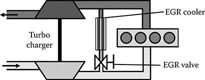
FIGURE 20.5 Engine layout of a high-pressure EGR system.
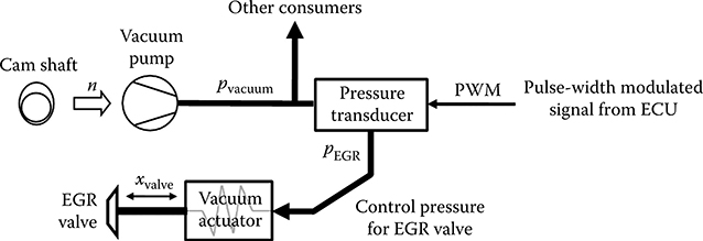
FIGURE 20.6 Method of actuation of the EGR valve.
The EGR system is subject to very high temperatures and exposed to deposits from the soot in the exhaust gas. This makes the system susceptible to failure. As EGR is used to lower NOx emissions, any deviation from the prescribed behavior will have a substantial impact on emission quality. A variety of fault possibilities is shown in Table 20.2.
It can be seen that different faults can lead to the same effect. In order to uniquely identify the cause for a fault, it is therefore not sufficient to solely detect it but also to determine particular characteristics that can be traced back to a failed component. There are many causalities in the engine behavior, which can be used for fault detection and identification, and often it is not clear even to the experienced engineer as to which ones are most relevant. For this reason, the HIL method is a valuable tool for the development of diagnostic functions as it reveals the causalities in a reproducible and cost-effective manner. A prerequisite is the usage of an appropriate RT engine model.
The model equations are derived by applying Newton’s Second Law to the EGR valve plate and valve stem. Besides the inertial force due to the mass of the moving valve, acting loads occur from the friction force, the return spring force, and the force as a result of the vacuum (see Figure 20.7). There are additional loads resulting from the pressure difference between inlet and exhaust port. These loads are neglected because they are small and can hardly be quantified once the valve has left its closed position.
Newton’s Second Law as applied with the forces acting on the valve
is used to determine the valve position x. The force from the vacuum actuator Fv depends on the pressure difference because of the vacuum pv, the spring force Fs depends on the valve position, the friction force FFr, implemented as a Coulomb– Stribeck function, depends on the valve velocity, and the mass m represents the sum of the moving masses.
TABLE 20.2
Various Faults Of An Egr System
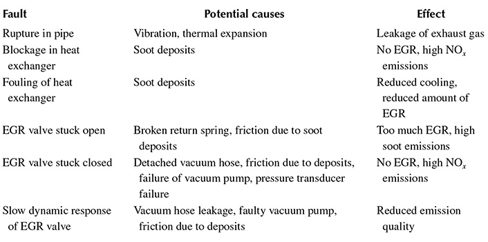
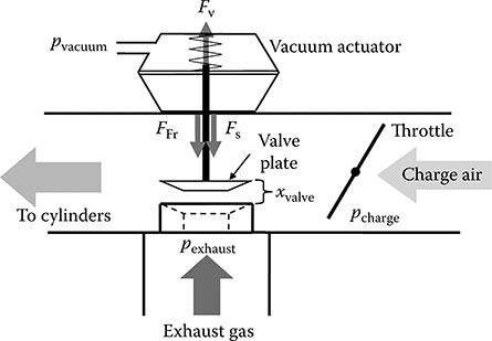
FIGURE 20.7 EGR valve system overview.
The EGR mass flow is calculated using the equation for an orifice
and depends on the gas states before and after the orifice, which are represented by density of the exhaust gas ρ, the pressure p, and the adiabatic exponent κ (Merker et al. 2006). The index 0 represents the upstream state of the orifice, and the index 1 represents the downstream state. The parameter A(x) is the flow area through the orifice dependent on valve lift. With the known values of EGR mass flow ṁEGR, intake air mass flow ṁ air, and their respective heat capacities c, the cylinder mass flow ṁcyl, and temperature Tcyl can be calculated:
The model is embedded in a mean-value model of a diesel engine as presented, for example, in Jensen et al. (1991) and in Guzzella and Amstutz (1998). The main advantage of the model is that faults can be easily simulated, which renders it very convenient for the testing of diagnostic functions on the HIL test bed. For simplicity, only the last three fault cases from Table 20.2 are considered further. These faults are introduced into the engine model by setting the valve lift to its minimum or maximum level, which represents the errors of the EGR valve stuck in a closed or open position, respectively. The increased friction is simulated by scaling the friction force by a factor of about 1.6, resulting in slow dynamic response of the valve.
Figure 20.8 shows a section of the cycle that was used for the OBD investigation. The engine speed and load were set independently as is possible on an engine test bed. The corresponding actuator signal for the EGR valve (PWMEGR) is shown in the top-left plot of Figure 20.8. The top-right plot of this figure shows the EGR valve lift for the fault cases. The legend of this figure is representative for the subsequent figures where it is not shown completely for the sake of clarity. The valve positions for the valve stuck in open and closed position, respectively, are visible. One can also clearly see the reduced dynamic behavior of the valve with increased friction of the valve shaft.
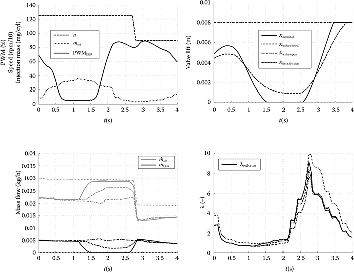
FIGURE 20.8 Simulated engine behavior during an induced fault occurrence.
The bottom two plots show the influence of the EGR valve faults on engine parameters. Their behavior matches the expectations well. For diagnostic functions, the parameters air mass flow and λ are of special interest as there are sensors for them in modern diesel engines that can be used for fault detection. The combustion-air ratio λ is defined as the actual air–fuel ratio divided by the stoichiometric air–fuel ratio. Model-based diagnostics (Isermann 2005) use the deviation of a sensor value from a model value, also referred to as a residual. The sensor value includes the effects of the fault while the model represents the nominal state as it is based on actuator signals and signals not affected by the fault. For diagnostics purposes, the goal is to gather as much information as possible about the fault from the residuals in order to identify the fault size, location, and time of occurrence. The residuals of the air mass flow and λ based on the simulation results given in Figure 20.8 are shown in Figure 20.9.
In creating diagnostic functions, fault patterns have to be defined and implemented as code. As this process is based on heuristic knowledge about the faults, the implementation of diagnostic functions for control units is an iterative process, which is ideally performed on a HIL test stand for reasons of cost and time savings. The diagnostic functions can be directly implemented on a prototype ECU and tested for correct operation. The residuals not only contain the information about the fault but also include model and measurement deviations and deviations due to component tolerances. It is the task of the diagnostic function to take these factors into account. In spite of careful design of the diagnostic function, final adjustments and validation with a real engine are still necessary, though.
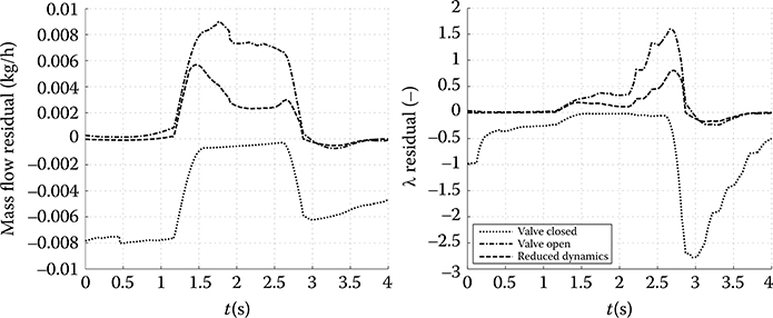
FIGURE 20.9 Residuals of mass flow and λ during the induced fault occurrence.
20.4.2 In-Cylinder Pressure Feedback Control
Changing legislation is forcing car manufacturers worldwide to reduce emissions and fuel consumption. Some manufacturers and suppliers are turning to in- cylinder pressure feedback control as a possibility to meet the upcoming emissions regulations, such as the EURO 6 and Tier II standards. Especially in transient operating conditions, engine emissions have much potential to be reduced by sophisticated strategies that precisely control the fuel injection and combustion process (Kuberczyk et al. 2010). Current developments in pressure sensors that can better withstand the harsh environment inside an engine are enabling new control strategies even without costly air mass flow sensors and, if otherwise present, NOx sensors (Klein 2009). In-cylinder pressure closed-loop control allows for an instantaneous modification of the fuel injection pattern based on the current operating conditions and the in-cylinder gas state for each cylinder. This allows for the compensation of unwanted disturbances and asymmetries between cylinders due to engine wear and variability of injectors and valves, hence optimizing the combustion of each cylinder individually (Nieuwstadt and Kolmanovsky 1999).
Employing HIL methods is a typical manner to develop these types of model-based control strategies. A HIL system requires a detailed RT simulation model providing the cylinder pressure depending on at least the current injection pattern and timing as well as the cylinder gas state, that is, temperature, pressure, and gas composition. The ECC approach presented in Section 20.3.1 is able to compute these values that describe the gas state in RT on standard computing hardware as shown for one operating point in Figure 20.10.
Commercial packages based on ECC, such as DYNA4Engine, ASM InCylinder, and GT Power RT, sample the pressure signal at a rate below 10 kHz and are able to capture all the prominent events such as ignition delay and start of ignition as well as the correct amount of energy released at the necessary time. The simulation step size must be significantly smaller than the commonly used 1 ms as evident when considering that 1 ms at an engine speed of 5000 rpm corresponds to 30 crank angle degrees. This requires a step size that is at least one order of magnitude smaller to be able to simulate the fuel injection and combustion sufficiently accurate for an ECU.
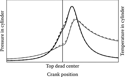
FIGURE 20.10 Normalized in-cylinder pressure and temperature around top dead center—measured (dashed) and simulated (solid).
In order to obtain a realistic time-resolved simulation of the in-cylinder pressure and temperature as shown, some practical issues arise:
Time delays: The sampling of signals in the I/O of the test rig delays signals an amount which corresponds to the characteristic time scales of the combustion process.
Sensors: Because of the extreme conditions inside the cylinder, the sensor degrades and its output drifts so that a model of the of the sensor behavior is mandatory.
Calibration: Some control schemes evaluate absolute values and not just the shape of the pressure curve, requiring correct calibration of the model.
However, the parts of the simulation model outside of the combustion process (e.g., the air path) normally only require a 1 ms step size, a fact exploited by means of a multirate simulation. Sampling rates are adapted to the eigenfrequencies of each subsystem. The task with the high sample rate would support the combustion process, the injection signals, and the cylinder pressure signal, whereas the slower task would apply to the rest of the model (Schuette and Ploeger 2007). RT simulation of heavy duty engines with a multitude of cylinders, for example, in marine applications, can be implemented by parallelization of the multirate model across multiple processors (DYNA4Engine 2009).
20.5 Future Developments
RT and HIL methods will certainly benefit from parallel computing, especially through the introduction of multicore processors. Particularly in the field of combustion engines, parallelization may pave the way toward RT simulation of one-dimensional gas dynamics, multizone cylinder models, and even CFD models that are beyond the current capabilities of standard RT hardware.
This will go well with the drastically increasing complexity of combustion engines due to emission relevant components such as selective catalytic reduction (SCR) catalytic converters or low pressure EGR, the usage of biofuels, and the demand for further improvement of fuel economy. The new era of electric and hybrid vehicles challenges the field of combustion engine control through a multitude of innovative topologies and use cases unknown to traditional automotive design. Simulation and particularly RT techniques will be able to close the gap in knowledge and experience while investigating the complex interactions between electronic, computational, and mechanical subsystems that will emerge from the integrated development of reliable and economical automotive systems.
References
AMESim. 2009. AMESim User Manual. Leuven, Belgium: LMS International.
ASCET-MD. 2009. ASCET V5.1 User Guide. Stuttgart, Germany: ETAS.
ASM InCylinder. 2006. ASM InCylinder Simulation Package. Paderborn, Germany: dSpace GmbH.
AVL FIRE. 2006. FIRE v8.5 Manual. Graz, Austria: AVL List GmbH.
Brenan, K. E., S. L. Campbell, and L. R. Petzold. 1989. Numerical Solution of Initial-Value Problems in Differential-Algebraic Equations. Amsterdam, The Netherlands: Elsevier.
Chung, T. J. 2003. Computational Fluid Dynamics. Cambridge: Cambridge University Press.
Douglass, B. P. 2004. Real Time UML: Advances in the UML for Real-Time Systems. 3rd ed. Boston, MA: Addison-Wesley.
Dymola. 2009. Dymola 7.4 User Guide. Paris, France: Dassault Systèmes.
DYNA4Engine. 2009. DYNA4Engine THEMOS User Guide. Munich, Germany: TESIS DYNAware GmbH.
Eich-Soellner, E., and C. Führer. 1998. Numerical Methods in Multibody Dynamics. Stuttgart, Germany: Teubner.
Elmqvist, H., M. Otter, and F. E. Cellier. 1995. “Inline Integration: A New Mixed Symbolic/ Numeric Approach for Solving Differential-Algebraic Equation Systems.” In Proceedings of the ESM’95, SCS European Simulation Multi-Conference, Prague, Czech Republic.
Gheorghiu, V. 1996. Modelle für die Echtzeitsimulation von Ottomotoren. Essen, Germany: Haus der Technik.
GT-Suite. 2009. GT-Suite V7.0. Westmont, IL: Gamma Technologies.
Guzzella, L., and A. Amstutz. 1998. “Control of Diesel Engines.” IEEE Control Systems Magazine 18(5): 53–71.
Hendricks, E., and S. Sorenson. 1990. “Mean Value Modelling of Spark Ignition Engines.” SAE Technical Paper 900616.
Heywood, J. B. 1989. Internal Combustion Engine Fundamentals. New York: McGraw-Hill Higher Education.
Isermann, R. 2005. “Model-Based Fault-Detection and Diagnosis—Status and Applications.” Annual Reviews in Control 29 (1): 71–85.
Izenman, A. J. 2008. Modern Multivariate Statistical Techniques: Regression, Classification, and Manifold Learning. New York: Springer.
Jensen, J.-P., A. F. Kristensen, S. C. Sorenson, N. Houbak, and E. Hendricks. 1991. “Mean Value Modeling of a Small Turbocharged Diesel Engine.” SAE Technical Paper 910070.
Klein, P. 2009. Zylinderdruckbasierte Füllungserfassung für Verbrennungsmotoren. PhD diss., Universität Siegen, Germany.
Kuberczyk, R., S. Dobler, B. Vahlensieck, and M. Mohr. 2010. “Reducing NOx and Particulate Emissions in Electrified Drivelines.” In Getriebe in Fahrzeugen. Friedrichshafen, Germany, June 22–23.
Lehmann, E. 2003. Time Partition Testing. PhD diss., Technische Universität Berlin, Germany.
Ljung, L. 1999. System Identification: Theory for the User. 2nd ed. Upper Saddle River, NJ: Prentice Hall.
Meder, G., A. Mitterer, H. Konrad, G. Krämer, and N. Siegl. 2007. “Development and Calibration of Model-Based Controller Functions by the Example of a Six Cylinder Engine with Full-Variable Valvetrain.” Automatisierungstechnik 55 (7): 339–45.
Merker, G., C. Schwarz, and R. Teichmann. 2011. Combustion Engines Development: Mixture Formation, Combustion, Emissions and Simulation. Berlin, Germany: Springer.
Modelica. 2010. Modelica Language Specification, V3.2. Linköping, Sweden: Modelica Association.
Moraal, P., and I. Kolmanovsky. 1999. “Turbocharger Modeling for Automotive Control Applications.” SAE Technical Paper 1999-01-0908.
Mosterman, P. J., and G. Biswas. 2002. “A Hybrid Modeling and Simulation Methodology for Dynamic Physical Systems.” Simulation: Transactions of the Society for Modeling and Simulation International 178 (1): 5–17.
Mosterman, P. J., S. Prabhu, A. Dowd, J. Glass, T. Erkkinen, J. Kluza, and R. Shenoy. 2005. “Embedded Real-Time Control via MATLAB, Simulink, and xPC Target.” In Handbook of Networked and Embedded Control Systems, edited by Dimitrios Hristu-Varsakelis and William S. Levine, 419–46. Boston, MA: Birkhäuser.
Mosterman, P. J., S. Prabhu, and T. Erkkinen. 2004. “An Industrial Embedded Control System Design Process.” In Proceedings of the Inaugural CDEN Design Conference (CDEN’04), 02B6-1 through 02B6-11, Montreal, Quebec, Canada, July 29–30, 2004.
Nieuwstadt, M. J., and I. Kolmanovsky. 1999. “Cylinder Balancing of Direct Injection Engines.” In Proceedings for the American Control Conference, San Diego, CA.
Papadimitriou, I., M. Warner, J. Silvestri, J. Lennblad, and S. Tabar. 2005. “Neural Network Based Fast-Running Engine Models for Control-Oriented Applications.” SAE Technical Paper 2005-01-0072.
Sargent, R. G. 2007. “Verification and Validation of Simulation Models.” In Proceedings of the 2007 Winter Simulation Conference, Washington, DC.
Schlesinger, S. et al. 1979. “Terminology for Model Credibility.” Simulation 34 3:101–5.
Schuette, H., and M. Ploeger. 2007. “Hardware-in-the-Loop Testing of Engine Control Units—A Technical Survey.” SAE Technical Paper 2007-01-0500.
Simulink. 2004. Using Simulink. Natick, MA: The MathWorks.
Vibe, I. I. 1970. Brennverlauf und Kreisprozess von Verbrennungsmotoren [German translation from Russian]. Berlin, Germany: VEB-Verlag Technik.
Vidyasagar, M. 1993. Nonlinear Systems Analysis. 2nd ed. Upper Saddle River, NJ: Prentice Hall.