We are still working with the company from the previous report. This company is a retail/distribution company that sells from their website, www.amazon.com, using an outside sales team (for bulk sales) and a brick and mortar store.

To improve cash flow, this company needs to evaluate how many times the accounts receivable is being paid and regenerated during the course of a year, and how many times the accounts payable will be paid and regenerated during the course of a year.

Monitoring these numbers gives a more accurate depiction of what is happening with collections and cash flow than from simply looking at an AR or AP Aged Trial Balance. This review is more robust because it takes sales and purchases into consideration.

Having large profits on your profit and loss statement does not pay the bills, cash does.

For this solution, we are going to build multiple pivot tables using Microsoft Excel 2013.

There are two parts to these steps. The first part is technical, containing steps that involve work in SQL Server. The second part is the actual building of the report. You may choose to obtain assistance with the technical part, especially if you do not have access to SQL Server.

Non-technical matter

With the SQL Server part completed in the previous section, let’s build a report:

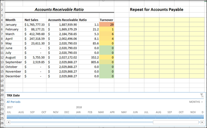
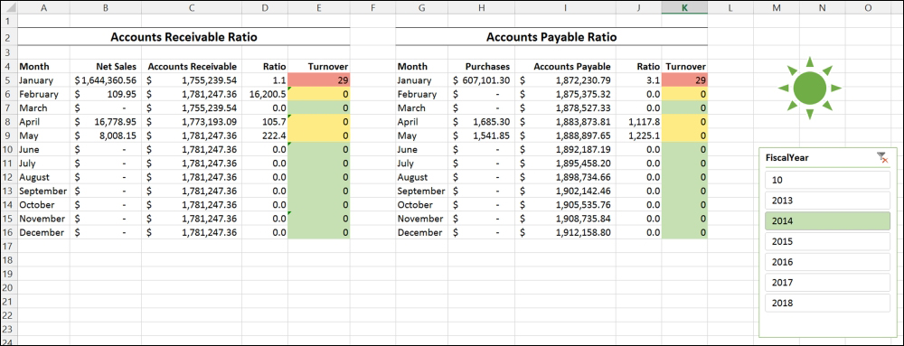
Know what you want. We’ve already completed this step, as shown in the following screenshot:

Tip

As always, we must know what we want our end result to look like before we start. Draw it on a paper or perform a “mock-up” in Excel. Starting with the end result in mind will save you many, many hours of time. We’ll say this over and over again because it’s that important! The preceding screenshot shows how we want our report to look.

Let’s make a connection to the GP data:

1. Open a blank workbook in Excel and from the menu bar choose Data. In the Get External Data portion of the ribbon, choose Existing Connections. Then, choose the appropriate view as the source and click on Open:
   

   Tip

   You can also repeat the entire steps of creating the data connection. If you do this, you will receive a message that the connection exists and do you want to overwrite. Overwriting is fine, especially since you are not changing the view itself.

Let’s build the first PivotTable:

1. In the Import Data window, select the PivotTable Report option and click on OK.
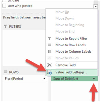
2. From PivotTable Fields list, drag FiscalPeriod to the ROWS area.
3. From the PivotTable Fields list, drag DebitNet to the Values area.
4. Choose the drop-down list next to Sum of DebitNet and select Value Field Settings:
   
5. Click on the Show Values As tab, from the drop-down list for Show values as and select Running Total In, making sure that the base period remains as FiscalPeriod. Then, click on the Number Format button:
   
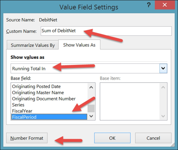
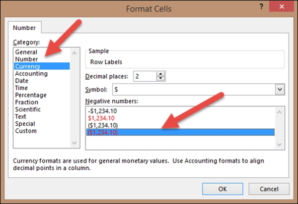
6. From the Format Cells window, select Currency as the category and change the negative numbers displayed if you like. Click on OK to close the Format Cells window, and then click on OK to close the Value Field Settings window:
   
7. From the PivotTable Fields list, drag Account Category Number to the Columns area.
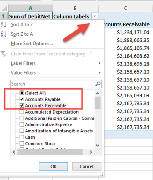
8. From the Column Labels drop-down list, with Select Multiple Items marked, unmark the Select All box and select only the categories that represent Accounts Payable and Accounts Receivable. Then, click on OK to close the drop-down list:
   
9. Save your Excel file, as you would with any other Excel file, to a secure area of the network.

Let’s build the second PivotTable:

1. Click on row one of the second available column (for us, that’s cell F1.) This is the start of our second PivotTable. We will be using this page for calculations only, not viewing.
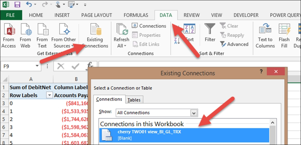
2. From the Excel menu, select Data and then select Get External Data. Choose the option that is part of the Connections in this Workbook section that references your view. Click on Open:
   
3. In the Import Data window, select the PivotTable Report option and click on OK.
4. In the PivotTable Fields list, drag FiscalPeriod to the ROWS area.
5. In the PivotTable Fields list, drag CreditNet to the VALUES area.
6. Choose the drop-down list next to Sum of CreditNet and select Value Field Settings.
7. Click on the Number Format button.
8. From the Format Cells window, select Currency as the category and change the negative numbers displayed if you like. Click on OK to close the Format Cells window.
9. In PivotTable Fields list, drag Account Category Number to the COLUMNS area.
10. From the Column Labels drop-down list, with Select Multiple Items marked, unmark the Select All box and select only the categories that represent sales and any sales-related account categories. Click on OK to close the drop-down list.
11. From the PivotTable Fields list, drag Series to the Filters area:
    
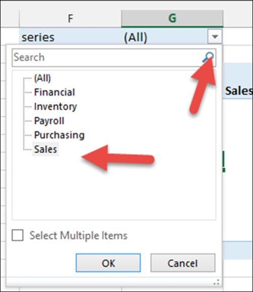
12. From the Column Labels drop-down list, with Select Multiple Items unmarked, select the Sales series. Click on OK to close the drop-down list.
13. Save the file as a precaution by navigating to File | Save

Let’s build the third PivotTable:

1. Click on row one of the second available column (for us, that’s cell I1.) This is the start of our final PivotTable. We will be using this page for calculations only, not viewing.
2. From the Excel menu, select Data and then select Get External Data. Choose the option that is part of the Connections in this workbook section that references your view. Click on Open.
3. In the Import Data window, select the PivotTable Report option and click on OK.
4. In the PivotTable Fields list, drag FiscalPeriod to the Rows area.
5. In the PivotTable Fields list, drag DebitNet to the Values area.
6. Choose the drop-down list next to Sum of DebitNet and select Value Field Settings.
7. Click on the Number Format button.
8. From the Format Cells window, select Currency as the category and change the negative numbers displayed if you like. Click on OK to close the Format Cells window.
9. In the PivotTable Fields list, drag Account Category Number to the Columns area.
10. From the Column Labels drop-down list, with Select Multiple Items unmarked, unmark the box for the category or categories that represent accounts payable-related accounts. Click on OK to close the drop-down list.
11. In the PivotTable Fields list, drag Series to the Filters area.
12. From the Column Labels drop-down list, with Select Multiple Items unmarked, select the Purchasing series. Click on OK to close the drop-down list.
13. Save the file as a precaution by navigating to File | Save.

Let’s create the AR Ratio side:

Tip

We now have three PivotTables. One represents AR and AP and the numbers roll forward, so each period should represent the YTD balance. One represents only transactions coded to sales and sales-related accounts that were originated in the sales series (sales order processing, receivables management, and invoicing.) The final one represents anything coded from the purchasing series, EXCEPT those lines that represent the accounts payable accounts.

Note that there is a “FiscalPeriod” “0”. This represents balances rolled forward from previous years.

1. Create a new worksheet on this workbook and name it Ratios:
   
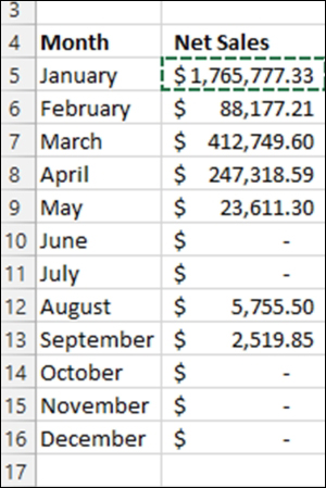
2. Click on cell A4. First, we’ll create the accounts receivable ratio. We’ll start entering the months here. Make sure to enter the column header Month in cell A4. Enter the months as they appear in your fiscal year. Our example is for a company with a calendar year as a fiscal year.
3. The next column will be Net Sales, so let’s enter this column header in cell B4. We want to reference the PivotTable we created on the Accounts worksheet for the corresponding month.

   Tip

   Two very important items to note:

   • We’ll need to use a custom GETPIVOTDATA formula for each month.
   • A month might not have activity in it, so we’ll need to account for this. If a month has no sales, there will be nothing to reference. If there is nothing to reference, we’ll receive a #REF message instead of a value.
4. Put your cursor in cell B5. Enter =IF(ISERROR()), rather than entering any further keys (including tab or enter), click on the Accounts worksheet, and click on the middle PivotTable (the one that represents sales) and click on the Sum of CreditNet field for “FiscalPeriod” 1. Then, type the following: “), 0,”, click again on the Accounts worksheet, and click in the middle PivotTable (the one that represents sales) and click on the Sum of CreditNet field for “FiscalPeriod” 1. Then, enter a final: “)”.

   Tip

   Our formula looks like the following:

   =IF(ISERROR(GETPIVOTDATA(“CreditNet”,Accounts!$F$4,“FiscalPeriod”,1)), 0, GETPIVOTDATA(“CreditNet”, Accounts!$F$4,”FiscalPeriod”,1))

   This formula indicates that if there is any error as a result of calling “FiscalPeriod” 1 Sales from the other worksheet, a 0 (zero) will be displayed; otherwise, “FiscalPeriod” 1 Sales will be displayed.

   No worries, the first month is always the most tedious. We can use the copy feature now to save us time.

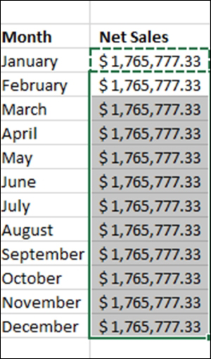
5. Copy cell B5 to the following months. You’ll see that the number is the same for each month. This is because the formula referenced “FiscalPeriod” 1, so each copy references that same month or period:
   
6. For each month, edit the formula changing the period number. The following is month February (for us, it is period 2) with the reference to month 2 highlighted:

   =IF(ISERROR(GETPIVOTDATA(“CreditNet”,Accounts!$F$4,“FiscalPeriod”,2)), 0, GETPIVOTDATA(“CreditNet”,Accounts!$F$4,”FiscalPeriod”,2))

   The following is month March with the reference to month 3 highlighted:

   =IF(ISERROR(GETPIVOTDATA(“CreditNet”,Accounts!$F$4,“FiscalPeriod”,3)), 0, GETPIVOTDATA(“CreditNet”,Accounts!$F$4,”FiscalPeriod”,3))

   Finish the months, making sure you make two period changes for each month as it’s listed twice in each formula.

   
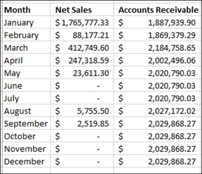
7. Click on cell C4 and enter the column header Accounts Receivable.
8. Now, for the Accounts Receivable Period balance, this is much easier, as the PivotTable has a running total as long as there is an amount in either the beginning period (0) or period 1. This means that every period will have an amount, so we can avoid that pesky =IF(ISERROR()) thing! Simply enter a “=”, and then find the correct field without tabbing or entering off cell C6. The cell we are looking for is the AR column of the first PivotTable for period 1.

   Our formula looks like the following:

   
9. Copy cell C5 for January (or your first fiscal period) to all months. We’ll need to change the formula again for months 2 through 12, but this time it’ll only be one change per formula. The following is our month 2 with the change highlighted:
   

   The following is our month 3 with the change highlighted.

   

   Once you get the point, continue for the remaining months/periods:

   
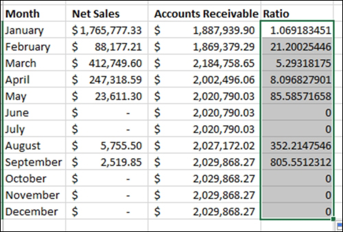
10. Click on cell D4 and enter the Ratio column header.
11. This is simply the Accounts Receivable balance (column C) divided by the Net Sales (Column B). However, there may be a month with no sales that would create an error in the calculation displaying the #DIV/0! error. To avoid this error, let’s use the same =IF(ISERROR()) formula we used for Net Sales. Your formula should look like the following:

    =IF(ISERROR(C5/B5), 0, (C5/B5))

    Copy this formula down the column for each month. Since we are referencing cell locations, the formula will copy with no editing. Hooray!

    
12. Click on cell E4 and enter the Turnover column header.
13. This is the formula that defines how long it takes for your entire accounts receivable to be paid off and a totally new accounts receivable to take its place. This formula is the number of days in a month divided by the ratio. Keep in mind that days in a month can vary, so we need to account for this. Our January formula looks like the following:

    =IF(ISERROR(31/D5), 0, (31/D5))

14. We’ll need to use the =IF(ISERROR()) formula to prevent divided by zero errors. Copy the January formula and edit the number of months where necessary.

    Tip

    September, April, June, and November have thirty days. All the rest have thirty-one, except February alone, which has twenty-eight days clear and twenty-nine in each leap year.

    If you are comfortable creating formulas that calculate the days in a month, by all means, include those.

Let’s create the AP Ratio side. Repeat the preceding steps for the AR Ratio with the following exceptions:

1. The Net Sales column will become the Purchases column and will reference the third PivotTable. Make sure to use the =IF(ISERROR()) formula.
2. The Accounts Receivable column will become the Accounts Payable column. Make sure to use the Accounts Payable column from the first PivotTable and not the Grand Total.
3. One extra step here is that we’ll need to take the entire formula and multiply it by “-1” to reverse the sign. Since we put Accounts Payable and Accounts Receivable in the same PivotTable, we’ll need to do this extra step. Our formula looks like the following, with the additional part highlighted:

   =(IF(ISERROR(GETPIVOTDATA(“DebitNet”,Accounts!$A$3,“Account Category Number”,”Accounts Payable”,“FiscalPeriod”,1)), 0, GETPIVOTDATA(“DebitNet”,Accounts!$A$3,”Account Category Number”,”Accounts Payable”,”FiscalPeriod”,1))*-1)
   

4. The Ratio will be the Accounts Payable column divided by the Purchases column. Make sure to use the =IF(ISERROR()) formula. You can simply copy the formulas from the AR side. Again, they just reference cell locations, so they’ll copy.
5. Copy the Turnover column from the AR side to the AP side. Again, they just reference cell locations, so they’ll copy too.

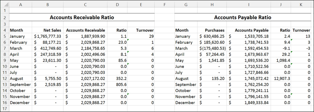
Let’s add the finishing touches:

1. Add column headers and your own special formatting skills to make this custom for you. After formatting, ours looks like the following:
   
2. Let’s add Slicers, so we can easily see various versions of the data with just a couple of mouse clicks.

   We’ll need to add a way for the user to select which fiscal period they are interested in. Let’s add a slicer like we did in the previous report.

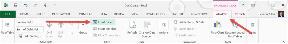
   Click on the Accounts worksheet and click on the first PivotTable. This will pull up the PIVOTTABLE TOOLS on the Excel menu. From the menu bar, select the ANALYZE tab and the Insert Slicer filter:

   
3. In the Insert Slicers window, select FiscalYear, and then click on OK.
4. From Slicer Tools on the Excel menu bar, select Options then Report Connections. Connect this slicer to all three PivotTables and click on OK to close the Report Connections window.
5. The FiscalYear slicer will appear on the Accounts worksheet. We want it to appear on the Ratios worksheet. We will simply use the cut and paste feature to move it. On the Accounts worksheet, click on the Slicer to select it; right-click and choose cut. Click on the Ratios worksheet and click below our work (we used cell A19); right-click and choose paste. Voila! It’s moved and active.
6. For our final formatting step, let’s add conditional formatting. We want to see, visually, in which months we are taking longer to collect and pay. We’ll start with the AR Turnover.

   Highlight all the months in column E (do not highlight the column header) with the mouse. For us, it is column E, cells 5-16.

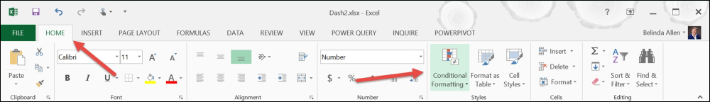
7. From the Excel menu, select Home, and from the Styles area on the ribbon, select Conditional Formatting:
   
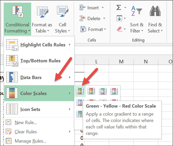
8. Choose Color Scales and the first option Green – Yellow – Red Color Scale:
   
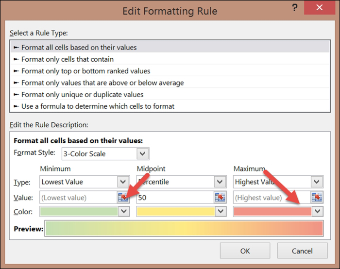
9. By default, the color scales show the highest numbers as good, so they are green, and the lowest numbers as bad, so they are red. We want these reversed; so with the cells still highlighted, from the Excel menu, select Home and from the Styles area on the ribbon, select Conditional Formatting. Choose the last option Manage Rules:
   
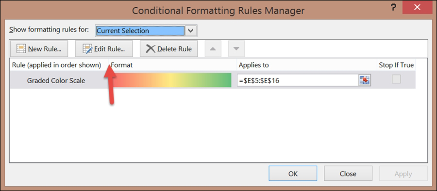
10. Click on the Edit Rule button. Change the colors of the Lowest Value (to green) and the Highest Value (to red). We used softer versions of red and green, so they are easier on the eyes. Click on OK to close the Edit Rule window, and click on OK to close the Conditional Formatting Rules Manager window:
    
11. Repeat this step for the AP side. You can also copy the AR Turnover column to the AP Turnover column.
12. At this point, you may choose to add a logo by choosing Insert from the Excel menu, and then from the illustrations area on the ribbon, choose Pictures.

    Tip

    You can also choose to have a date listed. We added the date formula for Today, so it always shows today’s date. We find this helpful to print. Another option for the date is to include a print date in the footer, so if you print, it’s already there.

13. If you choose to make this report automatically refresh, see the previous report for the steps. If you choose not to refresh automatically, you can refresh the data manually by choosing Data from the menu, and Refresh all from the connections area on the ribbon.
14. Save the file as a precaution by navigating to File | Save..
    

So, what does this report do for this company? These calculations are a uniform measure of how well you pay your bills and how well you collect on your invoices. Are you paying too fast? Too slow? Are you burning through cash? Are you good at collecting? A low accounts receivable may not mean that you collect well, rather it may mean that you do not invoice much. For those who decide to discuss financing with a bank, you should know that the bank will calculate this number and compare your numbers to others in your industry.