
Query designs that reduce resource use
Mechanisms to enhance the use of the plan cache
Reducing network overhead where possible
Techniques to reduce the transaction cost of a query
Avoiding Resource-Intensive Queries
Use the appropriate data types.
Test EXISTS over COUNT(*) to verify data existence.
Favor UNION ALL over UNION.
Ensure indexes are used in aggregation and sort operations.
Be cautious with local variables in batch queries.
Stored procedure names actually matter.
Use Appropriate Data Types
SQL Server supports a very large number of different data types. Also, SQL Server will automatically convert from one data type to another, depending of course on the data type. When this happens, it’s called an implicit conversion. This is a situation where SQL Server helps and makes your life easier, but at the cost of performance issues. To maintain your performance, use parameters, variables, and constants that are the same data type as the column you’re comparing.
Creating a test table with data and run queries against it
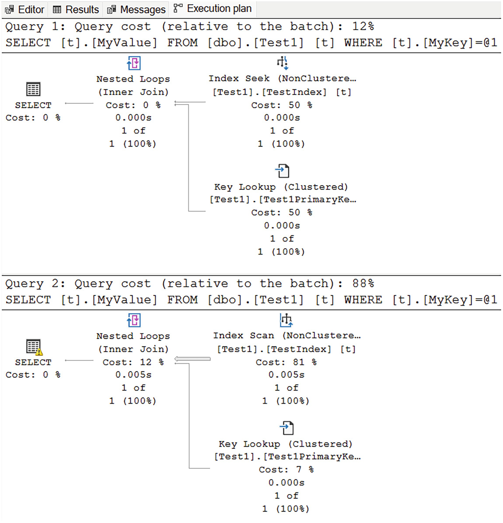
A diagram for query 1 has a query cost of 12% and begins from a non-clustered index seek at 50% cost and clustered key lookup at 50%, to nested loop, inner join at 0%, and select at 0%. A diagram for query 2 has a query cost of 88% and begins from a non clustered index scan at 81%.
Two execution plans showing implicit conversion at work
While the plan shapes are somewhat similar, two things should stand out. First, in the second plan, we can see a warning indicator on the first operator of the plan, the SELECT on the left. Second, again, in the second plan, we see that an Index Scan of the nonclustered index was done instead of the seek in the first plan. All of this was brought about by the need to convert the data type of the query from the NVARCHAR to VARCHAR because I set the hard-coded value through the use of “N” in front of the string definition at the end of Listing 15-1.
Because of the conversion, even though the result sets are identical, performance went from 137mcs on average to 5,927mcs. The reads went from 4 to 38.
Conversions are always done to the comparison value, whether it’s a variable, parameter, or hard-coded, not to the column. The comparison process has to use the values stored with the table or index, so the conversion is done to the other value.
As you can, while the implicit conversion process occurs simply, and in the background, it can be extremely problematic for performance. The best solution is to always match your hard-coded values, variables, and parameters to the column data type.
Test EXISTS over COUNT(*) to Verify Data Existence
Validating the existence of data through COUNT(*)
Validating data existence using EXISTS
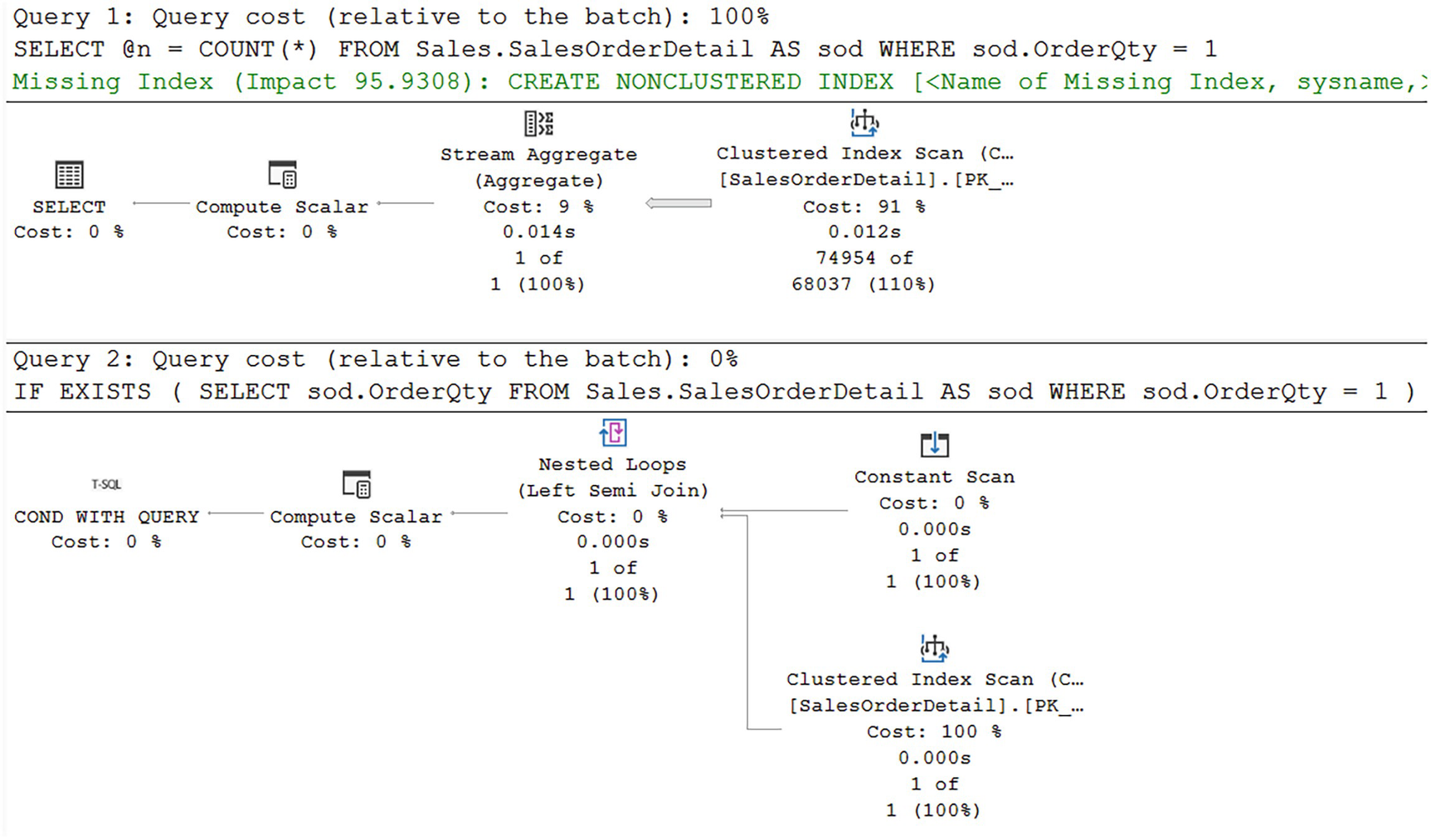
A diagram for query 1 has a cost of 100% and begins from a clustered index scan at 91% cost, to stream aggregate at 9%, and to compute scaler and select at 0% each. A diagram for query 2 has a cost of 0% and begins from constant and clustered index scans at 100% each.
Different execution plans between COUNT and EXISTS
While this may look like an obvious win, negative results, where the entire data set has to be scanned, may run the same or even slower. This is why I say test this approach in your systems. Clearly going from 1,248 reads down to 29 is a win.
Worth noting, the optimizer is suggesting a different index for the first query from Listing 15-3. Following that suggestion could enhance a little, but not as much as using EXISTS in this case.
Favor UNION ALL Over UNION
Combining result sets through UNION

A diagram has 3 non-clustered index seeks with costs of 12%, 12%, and 26%, and values 935 of 935, 926 of 926, and 3007 of 3007 given, respectively. Then 3 stream aggregates at 2%, 2%, and 7%, and values 935 of 905, 926 of 896, and 3007 of 2725, respectively.
Execution plan from a UNION query
In this case, the optimizer has chosen to satisfy the query through the use of the Stream Aggregate operations. You’ll note that each of the three data sets is retrieved through an Index Seek, but then they are aggregated, in order to eliminate duplicates, in the Stream Aggregate operations. The results of the aggregation are then combined through the two Merge Join operations.
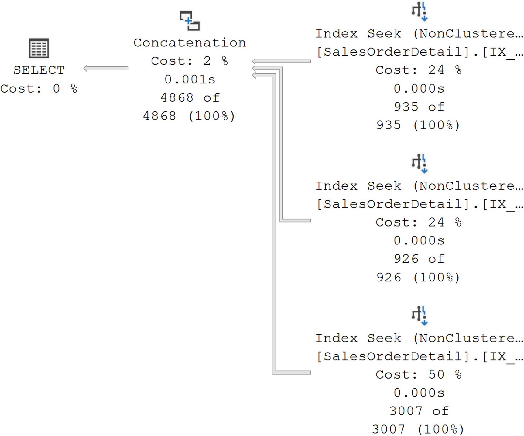
A diagram begins with 3 non-clustered index seeks on the right with costs of 24%, 24%, and 50%, and values 935 of 935, 926 of 926, and 3007 of 3007 given, respectively. Then concatenation on the left with values of 2% cost, 0.001 seconds.
An execution plan for UNION ALL
The aggregation operations are gone as are the joins. Instead, we’re left with just the data access through the Index Seek operations and then a combination of the data sets through the Concatenation operator. The plan is simpler, and the performance went from 5.1ms to 3.2ms. While it’s not a huge gain in this case, it may be as data sets grow. Interestingly, the reads stayed the same at 20 for both queries. The additional work was primarily taken up through CPU.
Ensure Indexes Are Used for Aggregate and Sort Operations
Looking for MIN UnitPrice
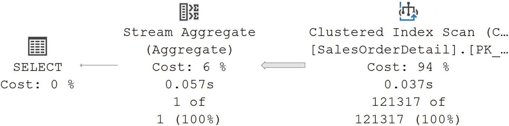
A diagram begins on the right with a clustered index scan with values of 94% cost, 0.037 seconds, and 121317 of 121317, given. From there it goes to a stream aggregate on the left with values of 6% cost, 0.057 seconds, and 1 of 1, and to select at 0%.
No supporting index for the aggregate query
Adding an index on the UnitPrice column
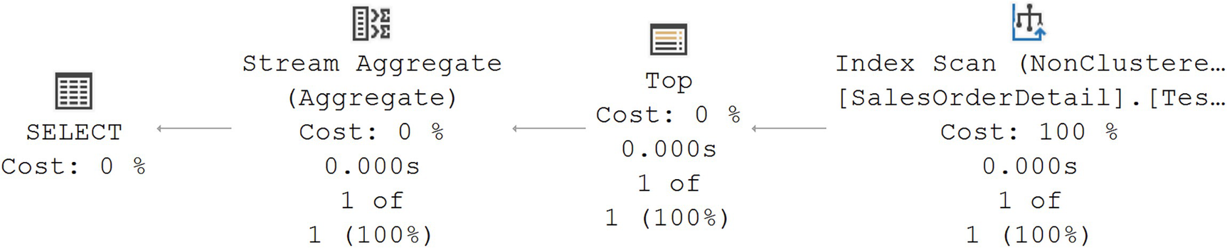
A diagram begins on the right with a non-clustered index scan with values of, 100% cost, 0.000 seconds, and 1 of 1, given. From there it goes to the top on the left with values of 0%, 0.000 seconds, and 1 of 1, stream aggregate with values of 0% cost, 0.000 seconds.
An index supports the query
While the plan looks more complex since it has more operations, the performance metrics speak for themselves. The index is scanned, but it’s a limited scan of a single row. The Top operator is to ensure that only one value is returned. The Stream Aggregate is merely a formality, validating the results.
Removing the test index
Be Cautious with Local Variables in a Batch Query
Using a local variable to pass values

A diagram begins on the right with a non-clustered index scan and clustered key lookup with values of 19% cost, 0.005 seconds, 48 of 3, 41%, 0.004 seconds, and 48 of 3 given, respectively.
Execution plan with a local variable
We’re filtering with the local variable on the ReferenceOrderID column of the TransactionHistory table. An Index Seek against a nonclustered index was used to satisfy the query. However, that means that additional values have to be pulled from the clustered index using the Key Lookup operation and a Nested Loops join. The rest of the data for the query comes from the Clustered Index Seek against the Product table and another Nested Loops join to pull them together.
Replacing the local variable
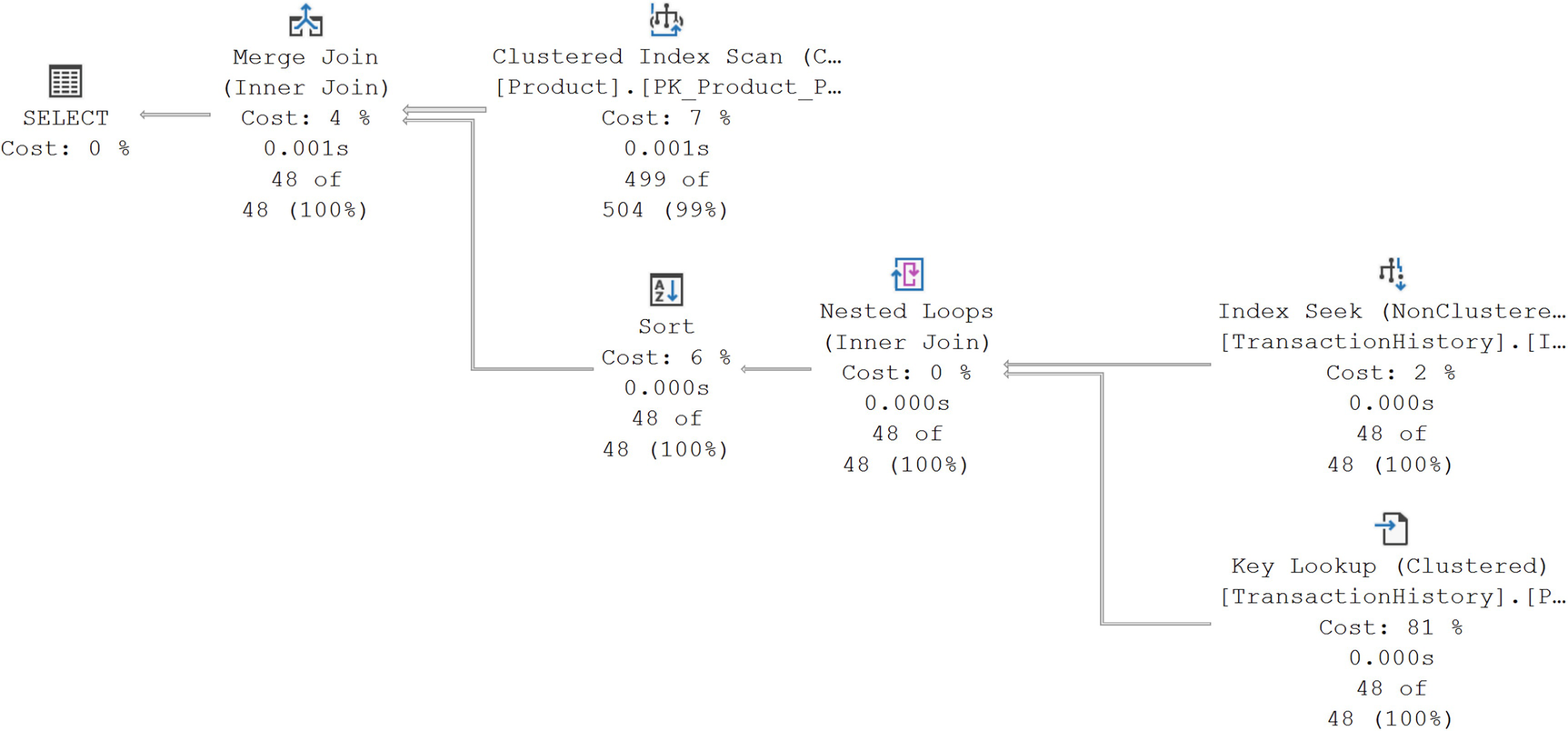
A diagram begins on the right with a non-clustered index scan and clustered key lookup with values of, 2% cost, 0.000 seconds, 48 of 8, and 81%, cost, 0.000 seconds, 48 of 48, given, respectively. Then nested loops, inner join at 0% cost, to a clustered index scan at 7%.
The execution plan changes with a hard-coded value
While we’re retrieving the exact same data set, the optimizer has made new choices in how best to satisfy the query. Some of the plan shape is the same. The data access against the TransactionHistory table is still through the nonclustered Index Seek and the Key Lookup. However, the rest of the plan is different. A Merge Join is used, as well as an Index Scan against the Product table’s clustered index. If you look at the properties of the Scan, you’ll find it’s an ordered scan, satisfying the need for the Merge Join to have ordered data. However, the other additional operator is the Sort, needed to get the data from the TransactionHistory table into order as well.
Listing 15-8 is considerably faster. However, Listing 15-9 uses fewer resources in terms of reads, 170 vs. 242. The key difference here is in the row estimates. If you look at Figures 15-7 and 15-8, you’ll notice that the number of rows estimated in Figure 15-7 is 3 while the number in Figure 15-8 is 48. You’ll also notice that in both cases, the actual number of rows returned as 48.
The real value for the row estimate is in the properties of the execution plan from Figure 15-7, 3.05628, rounded to the value we see of 3. The reason such an inaccurate estimate was used is because the value of a variable is not known to the optimizer at compile time. Because of this, the optimizer uses the density graph from the statistics, 2.694111E-05, and the number of rows, 113,443, and multiplies the two together, arriving at a row estimate of 3.05628.
The difference with the hard-coded value is that the optimizer can use the histogram to decide how many rows will be returned by the value used, 67620. That value from the histogram is 48, the actual number returned. The optimizer decided that performing 48 Index Seek operations through the Nested Loops join would be more expensive than doing an ordered scan of the index and sorting the results of the initial data from the TransactionHistory table.
However, in this case, the optimizer arrived at a plan that used fewer resources (Figure 15-8) but actually ran slower. This is one of those points where we have to start making choices when attempting to tune queries. If all we care about is speed of execution, in this case, using the local variable is faster. However, if our system was under load and potentially suffering from I/O issues, there’s a very good chance that the hard-coded value will perform better, since it performs fewer reads and will thus be in less conflict on the resources it uses.
I’m not advocating for hard-coded values, however. That leads to all sorts of code maintenance issues. Instead, you would want to explore the possibility of making the variable into a parameter so it can be sampled by the optimizer at compile time through parameter sniffing, although, again, that opens up issues as we explored in Chapter 13.
Sadly, there’s not always going to be a single, right answer when it comes to query tuning. However, gaining the knowledge of how, and more importantly, why, your queries are satisfied by the optimizer can help you make better choices.
Stored Procedure Names Actually Matter
The master database
The current database based on qualifiers (database name and/or owner)
In the current database using “dbo” as the schema if none is provided
The performance hit from this is tiny, almost to the point of not being able to measure it. However, on very active systems, you’re adding overhead that you simply don’t need to add. Another issue comes when you create a procedure in your local database, with the same name as a system procedure. Attempting to execute the query, especially if it has a different set of parameters, will simply cause an error.
Reducing Network Overhead Where Possible
Execute multiple queries in sets.
Use SET NOCOUNT.
To fully understand what I mean, we’ll drill down on these approaches.
Execute Multiple Queries in Sets
Everything is subject to testing, but generally, it’s a good approach to put sets of queries together in a batch or stored procedure. Rather than repeatedly connecting to the server, initiating a round trip across the network, call once and get the work done, returning what’s needed. You may have to ensure that your code can deal with multiple result sets. You also may need to ensure that you can consume JSON or other mechanisms of moving sets of data around, not simply single-row inserts or updates.
Use SET NOCOUNT
After every query in a batch or stored procedure, SQL Server will, by default, report the number of rows affected:
(<Number> row(s) affected)
Using the SET NOTCOUNT command
You can also set the NOCOUNT to OFF if you choose. Using this statement at the start of a set of queries or in a batch will not cause recompiles. It simply stops the reporting of those row counts. It’s a small thing, but it’s a good coding practice.
Techniques to Reduce Transaction Cost of a Query
Transactions are a fundamental part of how SQL Server protects the data in your system. Every action query—INSERT, UPDATE, DELETE, or MERGE—is performed as an atomic action in order to preserve the data in a consistent state, meaning data changes are successfully committed. This behavior cannot be disabled.
If the transition from one consistent state to another requires multiple database queries, then atomicity across the multiple queries should be maintained using explicitly defined database transactions. The old and new states of every atomic action are maintained in the transaction log (on the disk) to ensure durability, which guarantees that the outcome of an atomic action won’t be lost once it completes successfully. An atomic action during its execution is isolated from other database actions using database locks.
Reduce logging overhead.
Reduce lock overhead.
Reduce Logging Overhead
Inserting 10,000 rows of data
The DBCC command, SQLPERF, is a really simple way to look at the amount of log space consumed. At the start of the operation, I have a small log in AdventureWorks, about 72MB in size and only 4% full. Running Listing 15-11 takes 18 seconds and fills the log to about 58%. For a very small system like this, that’s a pretty massive impact.
Adding a transaction
Eliminating the WHILE loop
As with the simple addition of the transaction in Listing 15-12, we now have a single statement, so the percentage used of the log didn’t shift at all. And the performance improved even more, dropping down to about 310ms. We’ve gone from using 54% of the log to just almost nothing and 18 seconds to 310ms. It is possible to use fewer log resources.
However, a caution. Putting more work into a transaction can lead to a longer running transaction overall in some circumstances. That can lead to resource contention and blocking (which we’ll cover in Chapter 16). Also, longer transactions can add to the recovery time during a restore (although Accelerated Database Recovery certainly helps with this; for more, read the Microsoft documentation). As always, testing to validate how things work on your system is the best way to go.
Reduce Lock Overhead
By default, all T-SQL statements use some type of locking to isolate their work from that of other statements. Lock management adds performance overhead to a query. Another way to improve the performance of a query is reduce the number of locks necessary to satisfy a given query. Further, reducing the locking of one query improves the performance of other queries because they are then waiting less for those resources.
This is a very large topic which we’re going to drill down on in the next chapter. However, when talking about resource contention, I want to add a little detail on locking, here, in this chapter.
Code to supply a lock hint
The example in Listing 15-14 would supply a page level lock.
Mark the database as READONLY.
Use snapshot isolation.
Prevent SELECT statements from requesting a lock.
Mark the Database As READONLY
Changing the database to be READ_ONLY
Changing the database back to read/write
Use Snapshot Isolation
Changing the database isolation level
This will add overhead to the tempdb (again, except when using Accelerated Database Recovery). You can also set the isolation level in the connection string.
Prevent SELECT Statements from Requesting a Lock
Using the NOLOCK with a DELETE statement
You must know that the use of NOLOCK leads to dirty reads. Dirty reads can cause duplicate rows or missing rows. Therefore, NOLOCK should be considered only as a last resort to control locking. In fact, this is considered to be quite dangerous and will lead to improper results in queries. The best approach is to mark the database as read-only or use one of the snapshot isolation levels.
If you made any of the example changes to the database from this section, I recommend restoring from a backup.
Summary
Tuning queries is not simply about picking the right index and then ensuring that the code uses that index. As you can see, ensuring that you minimize the resources used by a query is also a big part of query tuning. Experimenting with different logical approaches to a given query can result in drastic performance enhancements, or simply reduce the resource use of a bottlenecked resource. When resources are in use, you will begin to experience performance hits caused by blocking on those resources. In the next chapter, we’ll examine how blocking affects SQL Server query performance.