
Chapter 7. Pulling apart the FROM clause
When can you ever have a serious query that doesn’t involve more than one table? Normalization is a wonderful thing and helps ensure that our databases have important characteristics such as integrity. But it also means using JOINs, because it’s unlikely that all the data we need to solve our problem occurs in a single table. Almost always, our FROM clause contains several tables.
In this chapter, I’ll explain some of the deeper, less understood aspects of the FROM clause. I’ll start with some of the basics, to make sure we’re all on the same page. You’re welcome to skip ahead if you’re familiar with the finer points of INNER, OUTER, and CROSS. I’m often amazed by the fact that developers the world over understand how to write a multi-table query, and yet few understand what they’re asking with such a query.
JOIN basics
Without JOINs, our FROM clause is incredibly simple. Assuming that we’re using only tables (rather than other constructs such as subqueries or functions), JOINs are one of the few ways that we can make our query more complicated. JOINs are part of day one in most database courses, and every day that follows is full of them. They are the simplest mechanism to allow access to data within other tables. We’ll cover the three types of JOINs in the sections that follow.
The INNER JOIN
The most common style of JOIN is the INNER JOIN. I’m writing that in capitals because it’s the keyword expression used to indicate the type of JOIN being used, but the word INNER is completely optional. It’s so much the most common style of JOIN that when we write only JOIN, we’re referring to an INNER JOIN.
An INNER JOIN looks at the two tables involved in the JOIN and identifies matching rows according to the criteria in the ON clause. Every INNER JOIN requires an ON clause—it’s not optional. Aliases are optional, and can make the ON clause much shorter and simpler to read (and the rest of the query too). I’ve made my life easier by specifying p and s after the table names in the query shown below (to indicate Product and ProductSubcategory respectively). In this particular example, the match condition is that the value in one column in the first table must be the same as the column in the second table. It so happens that the columns have the same name; therefore, to distinguish between them, I’ve specified one to be from the table p, and the other from the table s. It wouldn’t have mattered if I specified these two columns in the other order—equality operations are generally commutative, and it doesn’t matter whether I write a=b or b=a.
The query in listing 1 returns a set of rows from the two tables, containing all the rows that have matching values in their ProductSubcategoryID columns. This query, as with most of the queries in this chapter, will run on the AdventureWorks database, which is available as a sample database for SQL Server 2005 or SQL Server 2008.
Listing 1. Query to return rows with matching product subcategories
SELECT p.Name, s.Name
FROM Production.Product p
     JOIN
     Production.ProductSubcategory s
     ON p.ProductSubcategoryID = s.ProductSubcategoryID;
This query could return more rows than there are in the Product table, fewer rows, or the same number of rows. We’ll look at this phenomenon later in the chapter, as well as what can affect this number.
The OUTER JOIN
An OUTER JOIN is like an INNER JOIN except that rows that do not have matching values in the other table are not excluded from the result set. Instead, the rows appear with NULL entries in place of the columns from the other table. Remembering that a JOIN is always performed between two tables, these are the variations of OUTER JOIN:
- LEFT—Keeps all rows from the first table (inserting NULLs for the second table’s columns)
- RIGHT—Keeps all rows from the second table (inserting NULLs for the first table’s columns)
- FULL—Keeps all rows from both tables (inserting NULLs on the left or the right, as appropriate)
Because we must specify whether the OUTER JOIN is LEFT, RIGHT, or FULL, note that the keyword OUTER is optional—inferred by the fact that we have specified its variation. As in listing 2, I generally omit it, but you’re welcome to use it if you like.
Listing 2. A LEFT OUTER JOIN
SELECT p.Name, s.Name
FROM Production.Product p
     LEFT JOIN
     Production.ProductSubcategory s
     ON p.ProductSubcategoryID = s.ProductSubcategoryID;
The query in listing 2 produces results similar to the results of the last query, except that products that are not assigned to a subcategory are still included. They have NULL listed for the second column. The smallest number of rows that could be returned by this query is the number of rows in the Product table, as none can be eliminated.
Had we used a RIGHT JOIN, subcategories that contained no products would have been included. Take care when dealing with OUTER JOINs, because counting the rows for each subcategory would return 1 for an empty subcategory, rather than 0. If you intend to count the products in each subcategory, it would be better to count the occurrences of a non-NULL ProductID or Name instead of using COUNT(*). The queries in listing 3 demonstrate this potential issue.
Listing 3. Beware of COUNT(*) with OUTER JOINs
/* First ensure there is a subcategory with no corresponding products */
INSERT Production.ProductSubcategory (Name) VALUES ('Empty Subcategory'),

SELECT s.Name, COUNT(*) AS NumRows
FROM Production.ProductSubcategory s
     LEFT JOIN
     Production.Product p
     ON s.ProductSubcategoryID = p.ProductSubcategoryID
GROUP BY s.Name;

SELECT s.Name, COUNT(p.ProductID) AS NumProducts
FROM Production.ProductSubcategory s
     LEFT JOIN
     Production.Product p
     ON s.ProductSubcategoryID = p.ProductSubcategoryID
GROUP BY s.Name;
Although LEFT and RIGHT JOINs can be made equivalent by listing the tables in the opposite order, FULL is slightly different, and will return at least as many rows as the largest table (as no rows can be eliminated from either side).
The CROSS JOIN
A CROSS JOIN returns every possible combination of rows from the two tables. It’s like an INNER JOIN with an ON clause that evaluates to true for every possible combination of rows. The CROSS JOIN doesn’t use an ON clause at all. This type of JOIN is relatively rare, but it can effectively solve some problems, such as for a report that must include every combination of SalesPerson and SalesTerritory (showing zero or NULL where appropriate). The query in listing 4 demonstrates this by first performing a CROSS JOIN, and then a LEFT JOIN to find sales that match the criteria.
Listing 4. Using a CROSS JOIN to cover all combinations
SELECT p.SalesPersonID, t.TerritoryID, SUM(s.TotalDue) AS TotalSales
FROM Sales.SalesPerson p
     CROSS JOIN
     Sales.SalesTerritory t
     LEFT JOIN
     Sales.SalesOrderHeader s
     ON p.SalesPersonID = s.SalesPersonID
     AND t.TerritoryID = s.TerritoryID
GROUP BY p.SalesPersonID, t.TerritoryID;
Formatting your FROM clause
I recently heard someone say that formatting shouldn’t be a measure of good or bad practice when coding. He was talking about writing C# code and was largely taking exception to being told where to place braces. I’m inclined to agree with him to a certain extent. I do think that formatting guidelines should form a part of company coding standards so that people aren’t put off by the layout of code written by a colleague, but I think the most important thing is consistency, and Best Practices guides that you find around the internet should generally stay away from formatting. When it comes to the FROM clause, though, I think formatting can be important.
A sample query
The Microsoft Project Server Report Pack is a valuable resource for people who use Microsoft Project Server. One of the reports in the pack is a Timesheet Audit Report, which you can find at http://msdn.microsoft.com/en-us/library/bb428822.aspx. I sometimes use this when teaching T-SQL.
The main query for this report has a FROM clause which is hard to understand. I’ve included it in listing 5, keeping the formatting exactly as it is on the website. In the following sections, we’ll demystify it by using a method for reading FROM clauses, and consider ways that this query could have retained the same functionality without being so confusing.
Listing 5. A FROM clause from the Timesheet Audit Report
FROM     MSP_EpmResource
            LEFT OUTER JOIN MSP_TimesheetResource

            INNER JOIN MSP_TimesheetActual
               ON MSP_TimesheetResource.ResourceNameUID
                  = MSP_TimesheetActual.LastChangedResourceNameUID
               ON MSP_EpmResource.ResourceUID
                  = MSP_TimesheetResource.ResourceUID

            LEFT OUTER JOIN MSP_TimesheetPeriod

            INNER JOIN MSP_Timesheet
               ON MSP_TimesheetPeriod.PeriodUID
                  = MSP_Timesheet.PeriodUID

            INNER JOIN MSP_TimesheetPeriodStatus
               ON MSP_TimesheetPeriod.PeriodStatusID
                  = MSP_TimesheetPeriodStatus.PeriodStatusID

            INNER JOIN MSP_TimesheetStatus
               ON MSP_Timesheet.TimesheetStatusID
                  = MSP_TimesheetStatus.TimesheetStatusID
               ON MSP_TimesheetResource.ResourceNameUID
                  = MSP_Timesheet.OwnerResourceNameUID
The appearance of most queries
In the western world, our languages tend to read from left to right. Because of this, people tend to approach their FROM clauses from left to right as well.
For example, they start with one table:
FROM MSP_EpmResource
Then they JOIN to another table:
FROM     MSP_EpmResource
            LEFT OUTER JOIN MSP_TimesheetResource
               ON MSP_EpmResource.ResourceUID
                  = MSP_TimesheetResource.ResourceUID
And they keep repeating the pattern:
FROM     MSP_EpmResource
            LEFT OUTER JOIN MSP_TimesheetResource
               ON MSP_EpmResource.ResourceUID
                  = MSP_TimesheetResource.ResourceUID
            INNER JOIN MSP_TimesheetActual
               ON MSP_TimesheetResource.ResourceNameUID
                  = MSP_TimesheetActual.LastChangedResourceNameUID
They continue by adding on the construct JOIN table_X ON table_X.col = table_Y.col.
Effectively, everything is done from the perspective of the first table in the FROM clause. Some of the JOINs may be OUTER JOINs, some may be INNER, but the principle remains the same—that each table is brought into the mix by itself.
When the pattern doesn’t apply
In our sample query, this pattern doesn’t apply. We start with two JOINs, followed by two ONs. That doesn’t fit the way we like to think of our FROM clauses. If we try to rearrange the FROM clause to fit, we find that we can’t. But that doesn’t stop me from trying to get my students to try; it’s good for them to appreciate that not all queries can be written as they prefer. I get them to start with the first section (before the second LEFT JOIN):
FROM     MSP_EpmResource
            LEFT OUTER JOIN MSP_TimesheetResource

            INNER JOIN MSP_TimesheetActual
               ON MSP_TimesheetResource.ResourceNameUID
                  = MSP_TimesheetActual.LastChangedResourceNameUID
               ON MSP_EpmResource.ResourceUID
                  = MSP_TimesheetResource.ResourceUID
Many of my students look at this part and immediately pull the second ON clause (between MSP_EpmResource and MSP_TimesheetResource) and move it to before the INNER JOIN. But because we have an INNER JOIN applying to MSP_TimesheetResource, this would remove any NULLs that are the result of the OUTER JOIN. Clearly the logic has changed. Some try to fix this by making the INNER JOIN into a LEFT JOIN, but this changes the logic as well. Some move the tables around, listing MSP_EpmResource last, but the problem always comes down to the fact that people don’t understand this query. This part of the FROM clause can be fixed by using a RIGHT JOIN, but even this has problems, as you may find if you try to continue the pattern with the other four tables in the FROM clause.
How to read a FROM clause
A FROM clause is easy to read, but you have to understand the method. When I ask my students what the first JOIN is, they almost all say “the LEFT JOIN,” but they’re wrong. The first JOIN is the INNER JOIN, and this is easy to find because it’s the JOIN that matches the first ON. To find the first JOIN, you have to find the first ON. Having found it, you work backwards to find its JOIN (which is the JOIN that immediately precedes the ON, skipping past any JOINs that have already been allocated to an ON clause). The right side of the JOIN is anything that comes between an ON and its corresponding JOIN. To find the left side, you keep going backwards until you find an unmatched JOIN or the FROM keyword. You read a FROM clause that you can’t immediately understand this way:
- Find the first (or next) ON keyword.
- Work backwards from the ON, looking for an unmatched JOIN.
- Everything between the ON and the JOIN is the right side.
- Keep going backwards from the JOIN to find the left side.
- Repeat until all the ONs have been found.
Using this method, we can clearly see that the first JOIN in our sample query is the INNER JOIN, between MSP_TimesheetResource and MSP_TimesheetActual. This forms the right side of the LEFT OUTER JOIN, with MSP_EpmResource being the left side.
When the pattern can’t apply
Unfortunately for our pattern, the next JOIN is the INNER JOIN between MSP_TimesheetPeriod and MSP_Timesheet. It doesn’t involve any of the tables we’ve already brought into our query. When we continue reading our FROM clause, we eventually see that the query involves two LEFT JOINs, for which the right sides are a series of nested INNER JOINs. This provides logic to make sure that the NULLs are introduced only to the combination of MSP_TimesheetResource and MSP_TimesheetActual, not just one of them individually, and similarly for the combination of MSP_Time-sheetPeriod through MSP_TimesheetStatus.
And this is where the formatting becomes important. The layout of the query in its initial form (the form in which it appears on the website) doesn’t suggest that anything is nested. I would much rather have seen the query laid out as in listing 6. The only thing I have changed about the query is the whitespace and aliases, and yet you can see that it’s far easier to read.
Listing 6. A reformatted version of the FROM clause in listing 5
FROM
    MSP_EpmResource r
    LEFT OUTER JOIN
        MSP_TimesheetResource tr
        INNER JOIN
        MSP_TimesheetActual ta
        ON tr.ResourceNameUID = ta.LastChangedResourceNameUID
    ON r.ResourceUID = tr.ResourceUID
    LEFT OUTER JOIN
        MSP_TimesheetPeriod tp
        INNER JOIN
        MSP_Timesheet t
        ON tp.PeriodUID = t.PeriodUID
        INNER JOIN
        MSP_TimesheetPeriodStatus tps
        ON tp.PeriodStatusID = tps.PeriodStatusID
        INNER JOIN
        MSP_TimesheetStatus ts
        ON t.TimesheetStatusID = ts.TimesheetStatusID
    ON tr.ResourceNameUID = t.OwnerResourceNameUID
Laying out the query like this doesn’t change the importance of knowing how to read a query when you follow the steps I described earlier, but it helps the less experienced people who need to read the queries you write. Bracketing the nested sections may help make the query even clearer, but I find that bracketing can sometimes make people confuse these nested JOINs with derived tables.
Writing the FROM clause clearly the first time
In explaining the Timesheet Audit Report query, I’m not suggesting that it’s wise to nest JOINs as I just described. However, being able to read and understand a complex FROM clause is a useful skill that all query writers should have. They should also write queries that less skilled readers can easily understand.
Filtering with the ON clause
When dealing with INNER JOINs, people rarely have a problem thinking of the ON clause as a filter. Perhaps this comes from earlier days of databases, when we listed tables using comma notation and then put the ON clause predicates in the WHERE clause. From this link with the WHERE clause, we can draw parallels between the ON and WHERE clauses, but the ON clause is a different kind of filter, as I’ll demonstrate in the following sections.
The different filters of the SELECT statement
The most obvious filter in a SELECT statement is the WHERE clause. It filters out the rows that the FROM clause has produced. The database engine controls entirely the order in which the various aspects of a SELECT statement are applied, but logically the WHERE clause is applied after the FROM clause has been completed.
People also understand that the HAVING clause is a filter, but they believe mistakenly that the HAVING clause is used when the filter must involve an aggregate function. In actuality (but still only logically), the HAVING clause is applied to the groups that have been formed through the introduction of aggregates or a GROUP BY clause. It could therefore be suggested that the ON clause isn’t a filter, but rather a mechanism to describe the JOIN context. But it is a filter.
Filtering out the matches
Whereas the WHERE clause filters out rows, and the HAVING clause filters out groups, the ON clause filters out matches.
In an INNER JOIN, only the matches persist into the final results. Given all possible combinations of rows, only those that have successful matches are kept. Filtering out a match is the same as filtering out a row. For OUTER JOINs, we keep all the matches and then introduce NULLs to avoid eliminating rows that would have otherwise been filtered out. Now the concept of filtering out a match differs a little from filtering out a row.
When a predicate in the ON clause involves columns from both sides of the JOIN, it feels quite natural to be filtering matches this way. We can even justify the behavior of an OUTER JOIN by arguing that OUTER means that we’re putting rows back in after they’ve been filtered out. But when we have a predicate that involves only one side of the JOIN, things feel a bit different.
Now the success of the match has a different kind of dependency on one side than on the other. Suppose a LEFT JOIN has an ON clause like the one in listing 7.
Listing 7. Placing a predicate in the ON clause of an outer join
SELECT p.SalesPersonID, o.SalesOrderID, o.OrderDate
FROM
    Sales.SalesPerson p
    LEFT JOIN
    Sales.SalesOrderHeader o
    ON o.SalesPersonID = p.SalesPersonID
    AND o.OrderDate < '20020101';
For an INNER JOIN, this would be simple, and we’d probably have put the OrderDate predicate in the WHERE clause. But for an OUTER JOIN, this is different.
Often when we write an OUTER JOIN, we start with an INNER JOIN and then change the keyword to use LEFT instead of INNER (in fact, we probably leave out the word INNER). Making an OUTER JOIN from an INNER JOIN is done so that, for example, the salespeople who haven’t made sales don’t get filtered out. If that OrderDate predicate was in the WHERE clause, merely changing INNER JOIN to LEFT JOIN wouldn’t have done the job.
Consider the case of AdventureWorks’ SalesPerson 290, whose first sale was in 2003. A LEFT JOIN without the OrderDate predicate would include this salesperson, but then all the rows for that salesperson would be filtered out by the WHERE clause. This wouldn’t be correct if we were intending to keep all the salespeople.
Consider also the case of a salesperson with no sales. That person would be included in the results of the FROM clause (with NULL for the Sales.SalesOrderHeader columns), but then would also be filtered out by the WHERE clause.
The answer is to use ON clause predicates to define what constitutes a valid match, as we have in our code segment above. This means that the filtering is done before the NULLs are inserted for salespeople without matches, and our result is correct. I understand that it may seem strange to have a predicate in an ON clause that involves only one side of the JOIN, but when you understand what’s being filtered (rows with WHERE, groups with HAVING, and matches with ON), it should feel comfortable.
JOIN uses and simplification
To understand the FROM clause, it’s worth appreciating the power of the query optimizer. In this final part of the chapter, we’ll examine four uses of JOINs. We’ll then see how your query can be impacted if all these uses are made redundant.
The four uses of JOINs
Suppose a query involves a single table. For our example, we’ll use Production.Product from the AdventureWorks sample database. Let’s imagine that this table is joined to another table, say Production.ProductSubcategory. A foreign key relationship is defined between the two tables, and our ON clause refers to the ProductSubcategoryID column in each table. Listing 8 shows a view that reflects this query.
Listing 8. View to return products and their subcategories
CREATE VIEW dbo.ProductsPlus AS
SELECT p.*, s.Name as SubcatName
FROM
  Production.Product p
  JOIN
  Production.ProductSubcategory s
  ON p.ProductSubcategoryID = s.ProductSubcategoryID;
This simple view provides us with the columns of the Product table, with the name of the ProductSubcategory to which each product belongs. The query used is a standard lookup query, one that query writers often create.
Comparing the contents of this view to the Product table alone (I say contents loosely, as a view doesn’t store data unless it is an indexed view; it is simply a stored subquery), there are two obvious differences.
First, we see that we have an extra column. We could have made our view contain as many of the columns from the second table as we like, but for now I’m using only one. This is the first of the four uses. It seems a little trivial, but nevertheless, we have use #1: additional columns.
Secondly, we have fewer rows in the view than in the Product table. A little investigation shows that the ProductSubcategoryID column in Production.Product allows NULL values, with no matching row in the Production.ProductSubcategory table. As we’re using an INNER JOIN, these rows without matches are eliminated from our results. This could have been our intention, and therefore we have use #2: eliminated rows.
We can counteract this side effect quite easily. To avoid rows from Production. Product being eliminated, we need to convert our INNER JOIN to an OUTER JOIN. I have made this change and encapsulated it in a second view in listing 9, named dbo.ProductsPlus2 to avoid confusion.
Listing 9. View to return all products and their subcategories (if they exist)
CREATE VIEW dbo.ProductsPlus2 AS
SELECT p.*, s.Name AS SubcatName
FROM
  Production.Product p
  LEFT JOIN
  Production.ProductSubcategory s
  ON p.ProductSubcategoryID = s.ProductSubcategoryID;
Now when we query our view, we see that it gives us the same number of rows as in the Production.Product table.
JOINs have two other uses that we don’t see in our view.
As this is a foreign-key relationship, the column in Production.ProductSubcategory is the primary key, and therefore unique. There must be at most one matching row for each row in Production.Product—thereby not duplicating any of the rows from Production.Product. If Production.ProductSubcategory.ProductSubcategoryID weren’t unique, though, we could find ourselves using a JOIN for use #3: duplicated rows.
Please understand I am considering this only from the perspective of the first table, and the lack of duplications here is completely expected and desired. If we consider the query from the perspective of the second table, we are indeed seeing the duplication of rows. I am focusing on one table in order to demonstrate when the JOIN serves no direct purpose.
The fourth use is more obscure. When an OUTER JOIN is performed, rows that don’t have matches are persisted using NULL values for columns from the other table. In our second view above, we are using a LEFT JOIN, and NULL appears instead of the Name column from the Production.ProductSubcategory table. This has no effect on the fields from the table of products, but if we were using a RIGHT JOIN or FULL JOIN, and we had subcategories that contained no products allocated, we would find additional rows amongst our list of Products. That’s use #4: added NULL rows.
These four uses make up the entire functionality and purpose of JOINs: (1)gaining additional columns, (2)eliminating rows, (3)duplicating rows, and (4)adding NULL rows. The most commonly desired function would be the first one listed, but the other functions are just as valid. Perhaps we’re counting the number of times an event has occurred, and we take advantage of the duplication effect. Perhaps we want to consider only those records that have a match in another table, or perhaps we are using the added NULLs to find the empty subcategories. Whatever the business reason for performing the JOIN, everything comes back to these four uses.
Simplification using views
If listing the name of the ProductSubcategory with the product is often required, then a lookup similar to the one in the views created earlier could be functionality that is repeated frequently. Although a developer may consider this trivial and happily write out this JOIN notation as often as needed, there may be a temptation to use a view to simplify the query.
Consider the query in listing 10.
Listing 10. Query to return products and their subcategory
SELECT p.ProductID, p.Name, p.Color, s.Name as SubcatName
FROM
  Production.Product p
  LEFT JOIN
  Production.ProductSubcategory s
  ON p.ProductSubcategoryID = s.ProductSubcategoryID;
For every product in the Production.Product table, we are selecting the ProductID, Name, and Color, with the name of the subcategory to which it belongs. From our earlier discussion, we can see that the JOIN is not eliminating or duplicating rows, nor adding NULL rows, because of the LEFT JOIN, the uniqueness of s.ProductSubcategoryID, and the absence of a RIGHT/FULL JOIN, respectively.
Whereas it may seem useful to see that the SubcatName column is coming from a different table, the query could seem much simpler if it took advantage of our view dbo.ProductsPlus2, as created earlier:
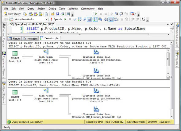
SELECT ProductID, Name, Color, SubcatName
FROM dbo.ProductsPlus2;
Again, a view doesn’t store any data unless it is indexed. In its non-indexed form, a view is just a stored subquery. You can compare the execution plans of these two queries, as shown in figure 1, to see that they are executed in exactly the same way.
Figure 1. Identical query plans demonstrating the breakdown of the view
The powerful aspect of this view occurs if we’re not interested in the SubcatName column:
SELECT ProductID, Name, Color
FROM dbo.ProductsPlus2;
Look at the execution plan for this query, as shown in figure 2, and you’ll see a vast difference from the previous one. Despite the fact that our view definition involves a second table, this table is not being accessed at all.
Figure 2. A much simpler execution plan involving only one table

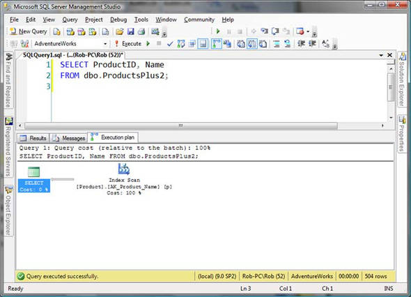
The reason for this is straightforward. The query optimizer examines the effects that the JOIN might have. When it sees that none apply (the only one that had applied was additional columns; ignoring the SubcatName column removes that one too), it realizes that the JOIN is not being used and treats the query as if the JOIN were not there at all. Furthermore, if we were not querying the Color column (as shown in figure 3), the query could take advantage of one of the nonclustered indexes on the Product table, as if we were querying the table directly.
Figure 3. A nonclustered index being used
As an academic exercise, I’m going to introduce a third view in listing 11—one that uses a FULL JOIN.
Listing 11. Using a FULL JOIN
CREATE VIEW dbo.ProductsPlus3 AS
SELECT p.*, s.Name as SubcatName
FROM
  Production.Product p
  FULL JOIN
  Production.ProductSubcategory s
  ON p.ProductSubcategoryID = s.ProductSubcategoryID;
This is far less useful, but I want to demonstrate the power of the query optimizer, so that you can better appreciate it and design your queries accordingly. In figure 4, notice the query plan that is being used when querying dbo.ProductsPlus3.
Figure 4. The ProductSubcategory table being used again
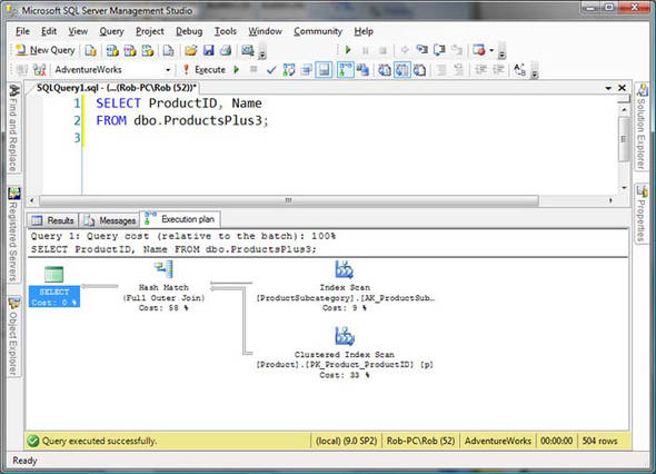
This time, when we query only the Name and ProductID fields, the query optimizer does not simplify out the Production.ProductSubcategory table. To find out why, let’s look at the four JOIN uses. No additional columns are being used from that table. The FULL JOIN prevents any elimination. No duplication is being created as the ProductSubcategoryID field is still unique in the second table. But the other use of a JOIN—the potential addition of NULL rows—could apply. In this particular case we have no empty subcategories and no rows are added, but the system must still perform the JOIN to satisfy this scenario.
Another way to ensure that NULL rows do not appear in the results of a query would be to use a WHERE clause:
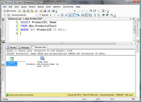
SELECT ProductID, Name
FROM dbo.ProductsPlus3
WHERE NOT ProductID IS NULL;
And now once more our execution plan has been simplified into a single-table query as shown in figure 5. The system detects that this particular use for a JOIN is made redundant regardless of whether it is being negated within the view or within the outer query. After all, we’ve already seen that the system treats a view as a subquery.
Figure 5. This execution plan is simpler because NULLs are not being introduced.
Regardless of what mechanism is stopping the JOIN from being used, the optimizer will be able to remove it from the execution plan if it is redundant.
How JOIN uses affect you
Although this may all seem like an academic exercise, there are important takeaways.
If the optimizer can eliminate tables from your queries, then you may see significant performance improvement. Recently I spent some time with a client who had a view that involved many tables, each with many columns. The view used OUTER JOINs, but investigation showed that the underlying tables did not have unique constraints on the columns involved in the JOINs. Changing this meant that the system could eliminate many more tables from the queries, and performance increased by orders of magnitude.
It is useful to be able to write queries that can be simplified by the optimizer, but if you can also make your queries simpler to understand, they’re probably quicker to write and easier to maintain. Why not consider using views that contain lookup information? Views that can be simplified can still wrap up useful functionality to make life easier for all the query writers, providing a much richer database to everyone.
Summary
We all need to be able to read and understand the FROM clause. In this chapter we’ve looked at the basics of JOINs, but also considered a methodology for reading more complex FROM clauses, and considered the ways that JOINs can be made redundant in queries.
I hope that after reading this chapter, you reexamine some of your FROM clauses, and have a new appreciation for the power of JOINs. In particular, I hope that part of your standard query writing process will include considering ways to allow JOINs to become redundant, using LEFT JOINs and uniqueness as demonstrated in the second half of this chapter.
About the author

Rob Farley is a Microsoft MVP (SQL) based in Adelaide, Australia, where he runs a SQL and BI consultancy called LobsterPot Solutions. He also runs the Adelaide SQL Server User Group, and regularly trains and presents at user groups around Australia. He holds many certifications and has made several trips to Microsoft in Redmond to help create exams for Microsoft Learning in SQL and .NET. His passions include Arsenal Football Club, his church, and his wife and three amazing children. The address of his blog is http://msmvps.com/blogs/robfarley, and his company website is at http://www.lobsterpot.com.au.