
Chapter 59. Incremental loads using T-SQL and SSIS
Back in the old days, when we used to walk to the card punch centers barefoot in the snow uphill both ways and carve our own computer chips out of wood, people performed incremental loads using the following steps:
1.
Open the source and destination files.
2.
Look at them.
3.
Where you see new rows in the source file, copy and paste them into the destination file.
4.
Where you see differences between rows that exist in both files, copy the source row and paste over the destination row.
Doubtless, some of you are thinking, “Andy, you nincompoop, no one cut and pasted production data—ever.” Oh really? I’d wager that in some department in every Global 1000 company, someone somewhere regularly cuts and pastes data into an Excel spreadsheet—even now. Read on to discover two ways to perform incremental loads in SQL Server the right way—using T-SQL and SQL Server Integration Services.
Some definitions
What, exactly, is an incremental load? An incremental load is a process where new and updated data from some source is loaded into a destination, whereas matching data is ignored. That last part about matching data is the key. If the data is identical in both source and destination, the best thing we can do is leave it be.
The chief advantage of an incremental load is time: generally speaking, it takes less time to perform an incremental load. The chief risk is misidentification. It’s possible to assign source rows to an incorrect status during the incremental load—the trickiest row status to identify is changed rows. Misidentified rows means a loss of data integrity. In the data warehouse field, less data integrity is often referred to as “bad.”
Incremental loads aren’t the only way to load data. Another popular method is called destructive loads. In a destructive load, the destination data is first removed—by deletion or, more often, truncation—before data is loaded from the source.
The chief advantage of a destructive load is data integrity. Think about it—if you’re simply copying the source into the destination, the opportunity to err drops dramatically. The chief disadvantage of a destructive load is the length of time it takes. Generally speaking, it takes longer to load all of the data when compared to loading a subset.
A T-SQL incremental load
Let’s look at a couple of ways to accomplish incremental loads. Our first example will be in Transact-SQL (T-SQL). Later, we’ll see an example using SQL Server 2005 Integration Services (SSIS 2005). To set up the T-SQL demo, use the following code to create two databases: a source database and a destination database (optional, but recommended):
CREATE DATABASE [SSISIncrementalLoad_Source]
CREATE DATABASE [SSISIncrementalLoad_Dest]
Now we need to create source and destination tables. We’ll start with creating the source table, as shown in listing 1.
Listing 1. Creating the tblSource source
USE SSISIncrementalLoad_Source
GO
CREATE TABLE dbo.tblSource
(ColID int NOT NULL
,ColA varchar(10) NULL
,ColB datetime NULL constraint df_ColB default (getDate())
,ColC int NULL
,constraint PK_tblSource primary key clustered (ColID))
The source table is named tblSource and contains the columns ColID, ColA, ColB, and ColC. For this example, make ColID the primary unique key. Next, we’ll create the destination table, as shown in listing 2.
Listing 2. Creating the tblDest destination
USE SSISIncrementalLoad_Dest
GO
CREATE TABLE dbo.tblDest
(ColID int NOT NULL
,ColA varchar(10) NULL
,ColB datetime NULL
,ColC int NULL)
This listing creates a destination table named tblDest with the columns ColID, ColA, ColB, and ColC. Next, we’ll load some test data into both tables for demonstration purposes, as shown in listing 3.
Listing 3. Loading data

As you can see, this listing populates the tables with some generic time and date information we’ll use in our query, shown in listing 4, to view the new rows.
Listing 4. Viewing new rows
SELECT s.ColID, s.ColA, s.ColB, s.ColC
FROM SSISIncrementalLoad_Source.dbo.tblSource s
LEFT JOIN SSISIncrementalLoad_Dest.dbo.tblDest d ON d.ColID = s.ColID
WHERE d.ColID IS NULL
This query should return the new row—the one loaded earlier with ColID = 2 and ColA = N. Why? The LEFT JOIN and WHERE clauses are the key. Left joins return all rows on the left side of the JOIN clause (SSISIncrementalLoad_Source.dbo. tblSource in this case) whether there’s a match on the right side of the JOIN clause (SSISIncrementalLoad_Dest.dbo.tblDest in this case) or not. If there’s no match on the right side, NULLs are returned. This is why the WHERE clause works: it goes after rows where the destination ColID is NULL. These rows have no match in the LEFT JOIN; therefore, they must be new.
Now we’ll use the T-SQL statement in listing 5 to incrementally load the row or rows.
Listing 5. Incrementally loading new rows
INSERT INTO SSISIncrementalLoad_Dest.dbo.tblDest
(ColID, ColA, ColB, ColC)
SELECT s.ColID, s.ColA, s.ColB, s.ColC
FROM SSISIncrementalLoad_Source.dbo.tblSource s
LEFT JOIN SSISIncrementalLoad_Dest.dbo.tblDest d ON d.ColID = s.ColID
WHERE d.ColID IS NULL
Although occasionally database schemas are this easy to load, most of the time you have to include several columns in the JOIN ON clause to isolate truly new rows. Sometimes you have to add conditions in the WHERE clause to refine the definition of truly new rows.
It’s equally crucial to identify changed rows. We’ll view the changed rows using the T-SQL statement in listing 6.
Listing 6. Isolating changed rows
SELECT d.ColID, d.ColA, d.ColB, d.ColC
FROM SSISIncrementalLoad_Dest.dbo.tblDest d
INNER JOIN SSISIncrementalLoad_Source.dbo.tblSource s ON s.ColID = d.ColID
WHERE (
(d.ColA != s.ColA)
OR (d.ColB != s.ColB)
OR (d.ColC != s.ColC)
)
Theoretically, you can try to isolate changed rows in many ways. But the only sure-fire way to accomplish this is to compare each field as we’ve done here. This should return the changed row we loaded earlier with ColID = 1 and ColA = C. Why? The INNER JOIN and WHERE clauses are to blame—again. The INNER JOIN goes after rows with matching ColIDs because of the JOIN ON clause. The WHERE clause refines the result set, returning only rows where ColA, ColB, or ColC don’t match and the ColIDs match.
This last bit is particularly important. If there’s a difference in any, some, or all of the rows (except ColID), we want to update it. To update the data in our destination, use the T-SQL shown in listing 7.
Listing 7. Updating the data
UPDATE d
SET
d.ColA = s.ColA
,d.ColB = s.ColB
,d.ColC = s.ColC
FROM SSISIncrementalLoad_Dest.dbo.tblDest d
INNER JOIN SSISIncrementalLoad_Source.dbo.tblSource s ON s.ColID = d.ColID
WHERE (
(d.ColA != s.ColA)
OR (d.ColB != s.ColB)
OR (d.ColC != s.ColC)
)
Extract, transform, and load (ETL) theory has a lot to say about when and how to update changed data. You’ll want to pick up a good book on the topic to learn more about the variations.
Note
Using SQL Server 2008, the new MERGE command can figure out which rows need to be inserted and which only need updating, and then perform the insert and update—all within a single command. Also new in SQL Server 2008 are the Change Tracking and Change Data Capture features which, as their names imply, automatically track which rows have been changed, making selecting from the source database much easier.
Now that we’ve looked at an incremental load using T-SQL, let’s consider how SQL Server Integration Services can accomplish the same task without all the hand-coding.
Incremental loads in SSIS
SQL Server Integration Services (SSIS) is Microsoft’s application bundled with SQL Server that simplifies data integration and transformations—and in this case, incremental loads. For this example, we’ll use SSIS to execute the lookup transformation (for the join functionality) combined with the conditional split (for the WHERE clause conditions) transformations.
Before we begin, let’s reset our database tables to their original state using the T-SQL code in listing 8.
Listing 8. Resetting the tables

With the tables back in their original state, we’ll create a new project using Business Intelligence Development Studio (BIDS).
Creating the new BIDS project
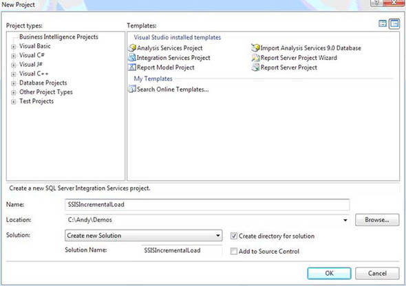
To follow along with this example, first open BIDS and create a new project. We’ll name the project SSISIncrementalLoad, as shown in figure 1. Once the project loads, open Solution Explorer, right-click the package, and rename Package1.dtsx to SSISIncrementalLoad.dtsx.
Figure 1. Creating a new BIDS project named SSISIncrementalLoad
When prompted to rename the package object, click the Yes button. From here, follow this straightforward series:
1.
From the toolbox, drag a data flow onto the Control Flow canvas. Double-click the data flow task to edit it.
2.
From the toolbox, drag and drop an OLE DB source onto the Data Flow canvas. Double-click the OLE DB Source connection adapter to edit it.
3.
Click the New button beside the OLE DB Connection Manager drop-down. Click the New button here to create a new data connection. Enter or select your server name. Connect to the SSISIncrementalLoad_Source database you created earlier. Click the OK button to return to the Connection Manager configuration dialog box.
4.
Click the OK button to accept your newly created data connection as the connection manager you want to define. Select dbo.tblSource from the Table drop-down.
5.
Click the OK button to complete defining the OLE DB source adapter.
Defining the lookup transformation
Now that the source adapter is defined, let’s move on to the lookup transformation that’ll join the data from our two tables. Again, there’s a standard series of steps in SSIS:
1.
Drag and drop a lookup transformation from the toolbox onto the Data Flow canvas.
2.
Connect the OLE DB connection adapter to the lookup transformation by clicking on the OLE DB Source, dragging the green arrow over the lookup, and dropping it.
3.
Right-click the lookup transformation and click Edit (or double-click the lookup transformation) to edit. You should now see something like the example shown in figure 2.
Figure 2. Using SSIS to edit the lookup transformation
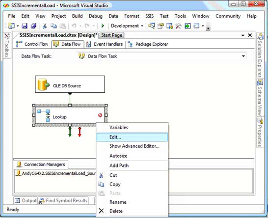
When the editor opens, click the New button beside the OLE DB Connection Manager drop-down (as you did earlier for the OLE DB source adapter). Define a new data connection—this time to the SSISIncrementalLoad_Dest database. After setting up the new data connection and connection manager, configure the lookup transformation to connect to dbo.tblDest. Click the Columns tab. On the left side are the columns currently in the SSIS data flow pipeline (from SSISIncrementalLoad_Source. dbo.tblSource). On the right side are columns available from the lookup destination you just configured (from SSISIncrementalLoad_Dest.dbo.tblDest).
We’ll need all the rows returned from the destination table, so check all the check boxes beside the rows in the destination. We need these rows for our WHERE clauses and our JOIN ON clauses.
We don’t want to map all the rows between the source and destination—only the columns named ColID between the database tables. The mappings drawn between the Available Input columns and Available Lookup columns define the JOIN ON clause. Multi-select the mappings between ColA, ColB, and ColC by clicking on them while holding the Ctrl key. Right-click any of them and click Delete Selected Mappings to delete these columns from our JOIN ON clause, as shown in figure 3.
Figure 3. Using the Lookup Transformation Editor to establish the correct mappings
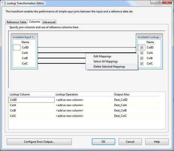
Add the text Dest_ to each column’s output alias. These rows are being appended to the data flow pipeline. This is so that we can distinguish between source and destination rows farther down the pipeline.
Setting the lookup transformation behavior
Next we need to modify our lookup transformation behavior. By default, the lookup operates similar to an INNER JOIN—but we need a LEFT (OUTER) JOIN. Click the Configure Error Output button to open the Configure Error Output screen. On the Lookup Output row, change the Error column from Fail Component to Ignore Failure. This tells the lookup transformation that if it doesn’t find an INNER JOIN match in the destination table for the source table’s ColID value, it shouldn’t fail. This also effectively tells the lookup to behave like a LEFT JOIN instead of an INNER JOIN. Click OK to complete the lookup transformation configuration.
From the toolbox, drag and drop a conditional split transformation onto the Data Flow canvas. Connect the lookup to the conditional split as shown in figure 4. Right-click the conditional split and click Edit to open the Conditional Split Transformation Editor. The Editor is divided into three sections. The upper-left section contains a list of available variables and columns. The upper-right section contains a list of available operations you may perform on values in the conditional expression. The lower section contains a list of the outputs you can define using SSIS Expression Language.
Figure 4. The Data Flow canvas shows a graphical view of the transformation.

Expand the NULL Functions folder in the upper-right section of the Conditional Split Transformation Editor, and expand the Columns folder in the upper-left section. Click in the Output Name column and enter New Rows as the name of the first output. From the NULL Functions folder, drag and drop the ISNULL( <<expression>> ) function to the Condition column of the New Rows condition. Next, drag Dest_ColID from the Columns folder and drop it onto the <<expression>> text in the Condition column. New rows should now be defined by the condition ISNULL( [Dest_ColID] ). This defines the WHERE clause for new rows—setting it to WHERE Dest_ColID Is NULL.
Type Changed Rows into a second output name column. Add the expression (ColA != Dest_ColA) || (ColB != Dest_ColB) || (ColC != Dest_ColC) to the Condition column for the Changed Rows output. This defines our WHERE clause for detecting changed rows—setting it to WHERE ((Dest_ColA != ColA) OR (Dest_ColB != ColB) OR (Dest_ColC != ColC)). Note that || is the expression for OR in SSIS expressions. Change the default output name from Conditional Split Default Output to Unchanged Rows.
It’s important to note here that the data flow task acts on rows. It can be used to manipulate (transform, create, or delete) data in columns in a row, but the sources, destinations, and transformations in the data flow task act on rows.
In a conditional split transformation, rows are sent to the output when the SSIS Expression Language condition for that output evaluates as true. A conditional split transformation behaves like a Switch statement in C# or Select Case in Visual Basic, in that the rows are sent to the first output for which the condition evaluates as true. This means that if two or more conditions are true for a given row, the row will be sent to the first output in the list for which the condition is true, and that the row will never be checked to see whether it meets the second condition. Click the OK button to complete configuration of the conditional split transformation.
Drag and drop an OLE DB destination connection adapter and an OLE DB command transformation onto the Data Flow canvas. Click on the conditional split and connect it to the OLE DB destination. A dialog box will display prompting you to select a conditional split output (those outputs you defined in the last step). Select the New Rows output. Next connect the OLE DB command transformation to the conditional split’s Changed Rows output. Your Data Flow canvas should appear similar to the example in figure 4.
Configure the OLE DB destination by aiming at the SSISIncrementalLoad_Dest.dbo.tblDest table. Click the Mappings item in the list to the left. Make sure the ColID, ColA, ColB, and ColC source columns are mapped to their matching destination columns (aren’t you glad we prepended Dest_ to the destination columns?). Click the OK button to complete configuring the OLE DB destination connection adapter. Double-click the OLE DB command to open the Advanced Editor for the OLE DB Command dialog box. Set the Connection Manager column to your SSISIncrementalLoad_Dest connection manager. Click on the Component Properties tab. Click the ellipsis (...) beside the SQLCommand property. The String Value Editor displays. Enter the following parameterized T-SQL statement into the String Value text box:
UPDATE dbo.tblDest
SET
ColA = ?
,ColB = ?
,ColC = ?
WHERE ColID = ?
The question marks in the previous parameterized T-SQL statement map by ordinal to columns named Param_0 through Param_3. Map them as shown here—effectively altering the UPDATE statement for each row:
UPDATE SSISIncrementalLoad_Dest.dbo.tblDest
SET
ColA = SSISIncrementalLoad_Source.dbo.ColA
,ColB = SSISIncrementalLoad_Source.dbo.ColB
,ColC = SSISIncrementalLoad_Source.dbo.ColC
WHERE ColID = SSISIncrementalLoad_Source.dbo.ColID
As you can see in figure 5, the query is executed on a row-by-row basis. For performance with large amounts of data, you’ll want to employ set-based updates instead. Click the OK button when mapping is completed. If you execute the package with debugging (press F5), the package should succeed.
Figure 5. The Advanced Editor shows a representation of the data flow prior to execution.

Note that one row takes the New Rows output from the conditional split, and one row takes the Changed Rows output from the conditional split transformation. Although not visible, our third source row doesn’t change, and would be sent to the Unchanged Rows output—which is the default Conditional Split output renamed. Any row that doesn’t meet any of the predefined conditions in the conditional split is sent to the default output.
Summary
The incremental load design pattern is a powerful way to leverage the strengths of the SSIS 2005 data flow task to transport data from a source to a destination. By using this method, you only insert or update rows that are new or have changed.
About the author

Andy Leonard is an architect with Unisys corporation, SQL Server database and integration services developer, SQL Server MVP, PASS regional mentor (Southeast US), and engineer. He’s a coauthor of several books on SQL Server topics. Andy founded and manages VSTeamSystemCentral.com and maintains several blogs there—Applied Team System, Applied Database Development, and Applied Business Intelligence—and also blogs for SQLBlog.com. Andy’s background includes web application architecture and development, VB, and ASP; SQL Server Integration Services (SSIS); data warehouse development using SQL Server 2000, 2005, and 2008; and test-driven database development.