
Chapter 56. Incorporating data profiling in the ETL process
When you work with data on a regular basis, it’s not uncommon to need to explore it. This is particularly true in the business intelligence and data warehousing field, because you may be dealing with new or changing data sources quite often. To work effectively with the data, you need to understand its profile—both what the data looks like at the detail level and from a higher aggregate level. In the case of small sets of data, you may be able to get a picture of the data profile by reviewing the detail rows. For larger sets of data, this isn’t practical, as there is too much information to easily hold in your head. Fortunately, SQL Server 2008 includes new functionality that makes this easier.
The data profiling tools in SQL Server Integration Services (SSIS) 2008 include a Data Profiling task and a Data Profile Viewer. The Data Profiling task is a new task for SSIS 2008. It can help you understand large sets of data by offering a set of commonly needed data profiling options. The Data Profile Viewer is an application that can be used to review the output of the Data Profiling task. Over the course of this chapter, I’ll introduce the Data Profiling task in the context of data warehousing and explain how it can be used to explore source data and how you can automate the use of the profile information in your extract, transform, and load (ETL) processes to make decisions about your data.
Why profile data?
Why should you be concerned with data profiling? In data warehousing, it is common to profile the data in advance to identify patterns in the data and determine if there are quality problems. Business intelligence applications often use data in new and interesting ways, which can highlight problems with the data simply because no one has looked at it in those ways before. The Data Profiling task helps identify these problems in advance by letting you determine what the data looks like statistically.
In many scenarios, the Data Profiling task will be used at the beginning of a data warehousing project to evaluate the source data prior to implementing ETL (or data integration) processes for it. When it is used this way, it can help identify problematic data in the sources. For example, perhaps the source database contains a Customer table with a State column, which should represent the U.S. state in which the customer resides. After profiling that table, you may discover that there are more than 50 distinct values in the column, indicating that you have either some incorrect states, some states have been entered in both their abbreviated form and spelled out, or possibly both. Once the problem data has been identified, you can design and incorporate the appropriate business rules in the ETL process to exclude or cleanse that data as it moves to the data warehouse, ensuring a higher quality of information in the warehouse. For the preceding example, this might be implemented by setting up a list of allowed values for the State column and matching incoming data against this list to validate it.
This upfront exploration of data and identification of problems is valuable, as it allows you to establish the rules that define what data can enter the data warehouse, and what data can be excluded, due to quality issues. Allowing bad data to enter the data warehouse can have a number of effects, all of them bad. For example, poor quality data in the warehouse will cause the users of the warehouse data to not trust it, or to potentially make bad decisions based on incorrect information. These rules are typically set up front, and may not be updated frequently (if at all) due to the complexities of changing production ETL processes. As data sources and business conditions change, these rules may become outdated. A better solution is to base some of the business rules on the current profile of the data, so that they remain dynamic and adjustable, even as the source data changes.
Changing production ETL processes
Why is modifying ETL processes so challenging? For one thing, any modifications usually require retesting the ETL. When you are dealing with hundreds of gigabytes—or terabytes—of data, that can be very time consuming. Also, any changes to the business rules in the ETL can impact historical data already in the warehouse. Determining whether to update historical information, or just change it moving forward, is a major decision in itself. If you do want to make changes to historical data, determining how to apply these updates can be complicated and typically involves multiple groups in the company (IT and any impacted business units) coming together to agree on an approach.
Now that we’ve discussed why data profiling is a good idea, let’s move on to the data profiling capabilities in SQL Server 2008.
Introduction to the Data Profiling task
The Data Profiling task is new for SSIS 2008. It has the capability to create multiple types of data profiles across any target tables you specify. Using it can be as simple as adding it to a package, selecting a SQL Server table, and picking one or more profiles to run against that table. Each profile returns a different set of information about the data in the target table.
First, we’ll cover the types of profiles that can be created, and then how you can work with them.
Types of profiles
The Data Profiling task supports eight different profiles. Five of these look at individual columns in a table, two of them look at multiple columns in the same table, and one looks at columns across two tables. A specific data profile works with specific data types (with some exceptions, which will be pointed out). In general, though, profiles work with some combination of string (char, nchar, varchar, nvarchar), integer (bit, tinyint, smallint, int, bigint), or date (datetime, smalldatetime, timestamp, date, time, datetime2, datetimeoffset) column data types. Most profiles do not work with binary types (such as text or image) or with non-integer numeric data.
The Column Length Distribution Profile
The Column Length Distribution profile provides the minimum and maximum lengths of values in a string column, along with a list of the distinct lengths of all values in the column and a count of rows that have that distinct length. For example, profiling a telephone number column (for U.S. domestic telephone numbers) where you expect numbers to be stored with no formatting should produce one value—a distinct length of 10. If any other values are reported, it indicates problems in the data.
The Column Null Ratio Profile
The Column Null Ratio profile is one of the exceptions in that it works with any type of data, including binary information. It reports the number of null values in a particular column. For example, profiling a column that is believed to always have a value because of rules enforced in the user interface may reveal that the rule isn’t always enforced.
The Column Pattern Profile
The Column Pattern profile only works on string columns and returns a list of regular expressions that match the values in the column. It may return multiple regular expressions, along with the frequency that the pattern applies to the data. For example, using this profile against a telephone number column might return the values d{10} (for numbers with no dashes—5555555555), d{3}-d{3}-d{4} (for numbers with dashes—555-555-5555), and d{3})d{3}-d{4} (for numbers with parentheses—(555)555-5555).
The Column Value Distribution Profile
The Column Value Distribution profile works on string, date, and numeric types (including money, decimal, float, real, and numeric). It returns the count of distinct values in a column, the list of the distinct values in a column, and the number of times each item is used. For example, this could be used to profile the distribution of product sales by product category by referencing a table of product sales that contains a column with product categories.
The Column Statistics Profile
The Column Statistics profile works on date and numeric types (including money, decimal, float, real, and numeric), but not on string data. It returns statistical information about the column: minimum and maximum values for date columns, and minimum, maximum, average, and standard deviation for numeric columns. A potential use for this is to profile the sale price of products to determine whether the data falls into acceptable ranges.
The Candidate Key Profile
The Candidate Key profile works with integer, string, and date data types. It evaluates a column or combination of columns to determine if they could be a key for the table. For example, this profile could be used against the combination of a name and telephone number column to determine if it could be used as key for the table. It is not uncommon to have primary keys that are generated values, using IDENTITY columns or the NEWSEQUENTIALID function, and you may need to determine whether there is a set of columns that represents the business or logical key for the data. You can use the Candidate Key profile to determine whether a proposed business key uniquely identifies each row in the table.
The Functional Dependency Profile
The Functional Dependency profile works with string, integer, and date data types. It evaluates how much the values in one column are determined by the values in another column or set of columns. It returns the determinant columns, the dependent column, and the strength of the dependency. This is useful for evaluating the data quality in one column based on another column. For example, a State column should have a strong functional dependency on a Zip Code column. If it doesn’t, it can indicate data-quality issues.
The Value Inclusion Profile
The Value Inclusion profile works with string, integer, and date data types. It determines whether a set of values in one table is present in another table. This can be used to determine whether a column is a good candidate to be a foreign key to another table, or to validate that all values present in one column exist in a reference table. For example, it can be used to validate that all state values in a table exist in a reference table of states.
Input to the task
Now that we’ve reviewed the available profiles, let’s take a look at how the task can be configured. You can configure a single Data Profiling task to generate multiple data profiles. Each profile can have its own reference to a connection manager and can target a single table (with the exception of the Value Inclusion profile, which targets two tables). For columns, you can use a wildcard so that it runs the same profile across all the columns in the table. Fortunately, the task is smart enough to only run profiles across columns with compatible data types. For example, using the Column Pattern profile with a wildcard for columns will only profile string columns.
As with most tasks in SSIS, there is an editor in the Business Intelligence Development Studio (BIDS) environment that allows you to set the properties for each profile. The Profile Requests page of the editor is pictured in figure 1. You can use the Quick Profile button located on the General page of the editor to easily define multiple profiles, for either a specific table or an entire database.
Figure 1. The Data Profiling Task Editor

The settings for the profiles are stored in the ProfileRequests property of the task, which is a collection of all the profile requests. Behind the scenes, the profile requests collection is converted to an XML document that conforms to the XML Schema located at http://schemas.microsoft.com/sqlserver/2008/DataDebugger/DataProfile.xsd. We’ll use this XML later in this chapter when we configure the task to be dynamic.
Output from the task
When the Data Profiling task is executed, it produces XML output that conforms to the DataProfile.xsd schema for the profile settings that are input. This XML can be directed to a file by using a file connection manager, or it can be stored in a variable inside the package. Typically, you will store the XML in a file if you are profiling data to be reviewed by a person at a later time, and plan on using the Data Profile Viewer application to review it. Storing the XML output in a variable is most often done when you want to use the profile information later in the same package, perhaps to make an automated decision about data quality.
The XML output includes both the profile requests (the input to the task) and the output from each profile requested. The format of the output varies depending on which profile generated it, so you will see different elements in the XML for a Column Null Ratio profile than you will for a Column Length Distribution profile. The XML contains a lot of information, and it can be difficult to sort through to find the information you are looking for. Fortunately, there is an easier user interface to use.
The Data Profile Viewer, shown in figure 2, provides a graphical interface to the data profile information. You can open XML files generated by the Data Profiling task in it and find specific information much more easily. In addition, the viewer represents some of the profile information graphically, which is useful when you are looking at large quantities of data. For example, the Column Length Distribution profile displays the count associated with specific lengths as a stacked bar chart, which means you can easily locate the most frequently used lengths.
Figure 2. Data Profile Viewer

The Data Profile Viewer lets you sort most columns in the tables that it displays, which can aid you in exploring the data. It also allows you to drill down into the detail data in the source system. This is particularly useful when you have located some bad data in the profile, because you can see the source rows that contain the data. This can be valuable if, for example, the profile shows that several customer names are unusually long. You can drill into the detail data to see all the data associated with these outlier rows. This feature does require a live connection to the source database, though, because the source data is not directly included in the data profile output.
One thing to be aware of with the Data Profile Viewer: not all values it shows are directly included in the XML. It does some additional work on the data profiles before presenting them to you. For example, in many cases it calculates the percentage of rows that a specific value in the profile applies to. The raw XML for the data profile only stores the row counts, not the percentages. This means that if you want to use the XML directly, perhaps to display the information on a web page, you may need to calculate some values manually. This is usually a straightforward task.
Constraints of the Data Profiling task
As useful as the Data Profiling task is, there are still some constraints that you need to keep in mind when using it. The first one most people encounter is in the types of data sources it will work with. The Data Profiling task requires that the data to be profiled be in SQL Server 2000 or later. This means you can’t use it to directly profile data in Oracle tables, Access databases, Excel spreadsheets, or flat files. You can work around this by importing the data you need into SQL Server prior to profiling it. In fact, there are other reasons why you may want the data in SQL Server in advance, which will be touched on in this section.
The Data Profiling task also requires that you use an ADO.NET connection manager. Typically, in SSIS, OLE DB connection managers are used, as they tend to perform better. This may mean creating two connection managers to the same database, if you need to both profile data and import it in the same package.
Using the Data Profile Viewer does require a SQL Server installation, because the viewer is not packaged or licensed as a redistributable component. It is possible to transform the XML output into a more user-friendly format by using XSL Transformations (XSLT) to translate it into HTML, or to write your own viewer for the information.
The task’s performance can vary greatly, depending both on the volume of data you are profiling and on the types of profiles you have requested. Some profiles, such as the Column Pattern profile, are resource intensive and can take quite a while on a large table. One way to address this is to work with a subset of the data, rather than the entire table. It’s important to get a representative sample of the data for these purposes, so that the data profile results aren’t skewed. This is another reason that having the data in SQL Server can be valuable. You can copy a subset of the data to another table for profiling, using a SELECT that returns a random sampling of rows (as discussed in “Selecting Rows Randomly from a Large Table” from MSDN: http://msdn.microsoft.com/en-us/library/cc441928.aspx). If the data is coming from an external source, such as a flat file, you can use the Row Sampling or Percentage Sampling components in an SSIS data flow to create a representative sample of the data to profile. Note that when sampling data, care must be taken to ensure the data is truly representative, or the results can be misleading. Generally it’s better to profile the entire data set.
Making the Data Profiling task dynamic
Why would you want to make the Data Profiling task dynamic? Well, as an example, think about profiling a new database. You could create a new SSIS package, add a Data Profiling task, and use the Quick Profile option to create profile requests for all the tables in the database. You’d then have to repeat these steps for the next new database that you want to profile. Or what if you don’t want to profile all the tables, but only a subset of them? To do this through the task’s editor, you would need to add each table individually. Wouldn’t it be easier to be able to dynamically update the task to profile different tables in your database?
Most tasks in SSIS can be made dynamic by using configurations and expressions. Configurations are used for settings that you wish to update each time a package is loaded, and expressions are used for settings that you want to update during the package execution. Both expressions and configurations operate on the properties of tasks in the package, but depending on what aspect of the Data Profiling task you want to change, it may require special handling to behave in a dynamic manner.
Changing the database
Because the Data Profiling task uses connection managers to control the connection to the database, it is relatively easy to change the database it points to. You update the connection manager, using one of the standard approaches in SSIS, such as an expression that sets the ConnectionString property, or a configuration that sets the same property. You can also accomplish this by overriding the connection manager’s setting at runtime using the /Connection switch of DTEXEC.
Bear in mind that although you can switch databases this way, the task will only work if it is pointing to a SQL Server database. Also, connection managers only control the database that you are connecting to, and not the specific tables. The profile requests in the task will still be referencing the original tables, so if the new database does not contain tables with the same names, the task will fail. What is needed is a way to change the profile requests to reference new tables.
Altering the profile requests
As noted earlier, you can configure the Data Profiling task through the Data Profiling Task Editor, which configures and stores the profile requests in the task’s ProfileRequests property. But this property is a collection object, and collection objects can’t be set through expressions or configurations, so, at first glance, it appears that you can’t update the profile requests.
Fortunately, there is an additional property that can be used for this on the Data Profiling task. This is the ProfileInputXml property, which stores the XML representation of the profile requests. The ProfileInputXml property is not visible in the Properties window in BIDS, but you can see it in the Property Expressions Editor dialog box, or in the Package Configuration Wizard’s property browser. You can set an XML string into this property using either an expression or a configuration. For it to work properly, the XML must conform to the DataProfile.xsd schema mentioned earlier.
Setting the ProfileInputXml property
So how can you go about altering the ProfileInputXml property to profile a different table? One way that works well is to create a string variable in the SSIS package to hold the table name (named TableName) and a second variable to hold the schema name (named SchemaName). Create a third variable that will hold the XML for the profile requests (named ProfileXML), and set the EvaluateAsVariable property of the Profile-XML variable to True. In the Expression property, you’ll need to enter the XML string for the profile, and concatenate in the table and schema variables.
To get the XML to use as a starting point, you can configure and run the Data Profile task with its output directed to a file. You’ll then need to remove the output information from the file, which can be done by removing all of the elements between the <DataProfileOutput> and <Profiles> tags, so that the XML looks similar to listing 1. You may have more or less XML, depending on how many profiles you configured the task for initially.
Listing 1. Data profile XML prior to making it dynamic

Once you have the XML, you need to change a few things to use it in an expression. First, the entire string needs to be put inside double quotes ("). Second, any existing double quotes need to be escaped, using a backslash (). For example, the ID attribute ID="StatisticsReq" needs to be formatted as ID="StatisticsReq". Finally, the profile requests need to be altered to include the table name variable created previously. These modifications are shown in listing 2.
Listing 2. Data profiling XML after converting to an expression

To apply this XML to the Data Profiling task, open the Property Expressions Editor by opening the Data Profiling Task Editor and going to the Expressions page. Select the ProfileInputXml property, and set the expression to be the ProfileXML variable. Now the task is set up so that you can change the target table by updating the SchemaName and TableName variables, with no modification to the task necessary.
Now that we’ve made the task dynamic, let’s move on to making decisions based on the output of the task.
Expressions in SSIS
Expressions in SSIS are limited to producing output no longer than 4,000 characters. Although that is enough for the example in this chapter, you may need to take it into account when working with multiple profiles. You can work around the limitation by executing the Data Profiling task multiple times, with a subset of the profiles in each execution to keep the expression under the 4,000-character limit.
Making data-quality decisions in the ETL
The Data Profiling task output can be used to make decisions about the quality of your data, and by incorporating the task output into your ETL process, you can automate these decisions. By taking things a little further, you can make these decisions self-adjusting as your data changes over time. We’ll take a look at both scenarios in the following sections.
Excluding data based on quality
Most commonly, the output of the Data Profiling task will change the flow of your ETL depending on the quality of the data being processed in your ETL. A simple example of this might be using the Column Null Ratio profile to evaluate a Customer table prior to extracting it from the source system. If the null ratio is greater than 30 percent for the Customer Name column, you might have your SSIS package set up to abort the processing and log an error message. This is an example of using data profiling information to prevent bad data from entering your data warehouse.
In situations like the preceding, though, a large percentage of rows that may have had acceptable data quality would also be excluded. For many data warehouses, that’s not acceptable. It’s more likely that these “hard” rules, such as not allowing null values in certain columns, will be implemented on a row-by-row basis, so that all acceptable data will be loaded into the warehouse, and only bad data will be excluded. In SSIS, this is often accomplished in the data flow by using Conditional Split transformations to send invalid data to error tables.
Adjusting rules dynamically
A more complex example involves using data profiling to establish what good data looks like, and then using this information to identify data of questionable quality. For example, if you are a retailer of products from multiple manufactures, your Product table will likely have the manufacturer’s original part number, and each manufacturer may have its own format for part numbers. In this scenario, you might use the Column Pattern profile against a known good source of part numbers, such as your Product table or your Product master, to identify the regular expressions that match the part numbers. During the execution of your ETL process, you could compare new incoming part numbers with these regular expressions to determine if they match the known formats for part numbers. As new products are added to the known good source of part numbers, new patterns will be included in the profile, and the rule will be adjusted dynamically.
It’s worth noting that this type of data-quality check is often implemented as a “soft” rule, so the row is not prohibited from entering the data warehouse. After all, the manufacturer may have implemented a new part-numbering scheme, or the part number could have come from a new manufacturer that is not in the Product dimension yet. Instead of redirecting the row to an error table, you might set a flag on the row indicating that there is a question as to the quality of the information, but allow it to enter the data warehouse anyway. This would allow the part number to be used for recording sales of that product, while still identifying a need for someone to follow up and verify that the part number is correct. Once they have validated the part number, and corrected it if necessary, the questionable data flag would be removed, and that product could become part of the known good set of products. The next time that you generate a Column Pattern profile against the part numbers, the new pattern will be included, and new rows that conform to it will no longer be flagged as questionable.
As mentioned earlier, implementing this type of logic in your ETL process can allow it to dynamically adjust data-quality rules over time, and as your data quality gets better, the ETL process will get better at flagging questionable data.
Now let’s take a look at how to use the task output in the package.
Consuming the task output
As mentioned earlier, the Data Profiling task produces its output as XML, which can be stored in a variable or a file. This XML output will include both the profile requests and the output profiles for each request.
Capturing the output
If you are planning to use the output in the same package that the profiling task is in, you will usually want to store the output XML in a package variable. If the output will be used in another package, how you store it will depend on how the other package will be executed. If the second package will be executed directly from the package performing the profiling through an Execute Package task, you can store the output in a variable and use a Parent Package Variable configuration to pass it between the packages. On the other hand, if the second package will be executed in a separate process or at a different time, storing the output in a file is the best option.
Regardless of whether the output is stored in a variable or a file, it can be accessed in a few different ways. Because the output is stored as XML, you can make use of the XML task to use it in the control flow, or the XML source to use it in the data flow. You can also use the Script task or the Script component to manipulate the XML output directly using .NET code.
Using SSIS XML functionality
The XML task is provided in SSIS so that you can work with XML in the control flow. Because the Data Profiling task produces XML, it is a natural fit to use the XML task to process the data profile output. Primarily, the XSLT or XPATH operations can be used with the profile XML.
The XSLT operation can be used to transform the output into a format that’s easier to use, such as filtering the profile output down to specific profiles that you are interested in, which is useful if you want to use the XML source to process it. The XSLT operation can also be used to remove the default namespace from the XML document, which makes using XPATH against it much easier.
XPATH operations can be used to retrieve a specific value or set of nodes from the profile. This option is illustrated by the Trim Namespaces XML task in the sample package that accompanies this chapter, showing how to retrieve the null count for a particular column using XPATH.
Note
The sample package for this chapter can be found on the book’s website at http://www.manning.com/SQLServerMVPDeepDives.
New to XML?
If you are new to XML, the preceding discussion may be a bit confusing, and the reasons for taking these steps may not be obvious. If you’d like to learn more about working with XML in SSIS, please review these online resources:
- General XML information: http://msdn.microsoft.com/en-us/xml/default.aspx
- Working with XML in SSIS: http://blogs.msdn.com/mattm/archive/tags/XML/default.aspx
In the data flow, the XML source component can be used to get information from the Data Profiling task output. You can do this in two ways, one of which is relatively straightforward if you are familiar with XSLT. The other is more complex to implement but has the benefit of not requiring in-depth XSLT knowledge.
If you know XSLT, you can use an XML task to transform and simplify the Data Profiling task output prior to using it in the XML source, as mentioned previously. This can help avoid having to join multiple outputs from the XML source, which is discussed shortly.
If you don’t know XSLT, you can take a few additional steps and use the XML source directly against the Data Profiling task output. First, you must provide an .XSD file for the XML source, but the .XSD published by Microsoft at http://schemas.microsoft.com/sqlserver/2008/DataDebugger/DataProfile.xsd is too complex for the XML source. Instead, you will need to generate a schema using an existing data profile that you have saved to a file. Second, you have to identify the correct outputs from the XML source. The XML source creates a separate output for each distinct element type in the XML: the output from the Data Profiling task includes at least three distinct elements for each profile you include, and for most profiles it will have four or more. This can lead to some challenges in finding the appropriate output information from the XML source. Third, because the XML source does not flatten the XML output, you have to join the multiple outputs together to assemble meaningful information. The sample package on the book’s website (http://www.manning.com/SQLServerMVPDeepDives) has an example of doing this for the Column Pattern profile. The data flow is shown in figure 3.
Figure 3. Data flow to reassemble a Column Pattern profile
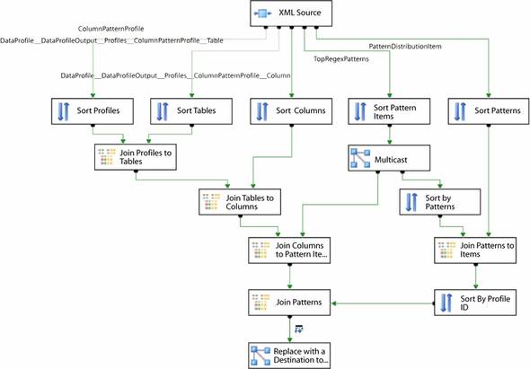
In the data flow shown in figure 3, the results of the Column Pattern profile are being transformed from a hierarchical structure (typical for XML) to a flattened structure suitable for saving into a database table. The hierarchy for a Column Pattern profile has five levels that need to be used for the information we are interested in, and each output from the XML source includes one of these levels. Each level contains a column that ties it to the levels used below it. In the data flow, each output from the XML source is sorted, so that consistent ordering is ensured. Then, each output, which represents one level in the hierarchical structure, is joined to the output representing the next level down in the hierarchy. Most of the levels have a ColumnPattern-Profile_ID, which can be used in the Merge Join transformation to join the levels, but there is some special handling required for the level representing the patterns, as they need to be joined on the TopRegexPatterns_ID instead of the ColumnPattern-Profile_ID. This data flow is included in the sample package for this chapter, so you can review the logic if you wish.
Using scripts
Script tasks and components provide another means of accessing the information in the Data Profiling task output. By saving the output to a package variable, you make it accessible within a Script task. Once in the Script task, you have the choice of performing direct string manipulation to get the information you want, or you can use the XmlDocument class from the System.Xml namespace to load and process the output XML. Both of these approaches offer a tremendous amount of flexibility in working with the XML. As working with XML documents using .NET is well documented, we won’t cover it in depth here.
Another approach that requires scripting is the use of the classes in the DataProfiler.dll assembly. These classes facilitate loading and interacting with the data profile through a custom API, and the approach works well, but this is an undocumented and unsupported API, so there are no guarantees when using it. If this doesn’t scare you off, and you are comfortable working with unsupported features (that have a good chance of changing in new releases), take a look at “Accessing a data profile programmatically” on the SSIS Team Blog (http://blogs.msdn.com/mattm/archive/2008/03/12/accessing-a-data-profile-programmatically.aspx) for an example of using the API to load and retrieve information from a data profile.
Incorporating the values in the package
Once you have retrieved values from the data profile output, using one of the methods discussed in the previous sections, you need to incorporate it into the package logic. This is fairly standard SSIS work.
Most often, you will want to store specific values retrieved from the profile in a package variable, and use those variables to make dynamic decisions. For example, consider the Column Null Ratio profiling we discussed earlier. After retrieving the null count from the profile output, you could use an expression on a precedence constraint to have the package stop processing if the null count is too high.
In the data flow, you will often use Conditional Split or Derived Column transformations to implement the decision-making logic. For example, you might use the Data Profiling task to run a Column Length Distribution profile against the product description column in your Product table. You could use a Script task to process the profile output and determine that 95 percent of your product descriptions fall between 50 and 200 characters. By storing those boundary values in variables, you could check for new product descriptions that fall outside of this range in your ETL. You could use the Conditional Split transformation to redirect these rows to an error table, or the Derived Column transformation to set a flag on the row indicating that there might be a data-quality issue.
Some data-quality checking is going to require more sophisticated processing. For the Column Pattern checking scenario discussed earlier, you would need to implement a Script component in the data flow that can take a list of regular expressions and apply them against the column that you wanted to check. If the column value matched one or more of the regular expressions, it would be flagged as OK. If the column value didn’t match any of the regular expressions, it would be flagged as questionable, or redirected to an error table. Listing 3 shows an example of the code that can perform this check. It takes in a delimited list of regular expression patterns, and then compares each of them to a specified column.
Listing 3. Script component to check column values against a list of patterns
public class ScriptMain : UserComponent
{
    List<Regex> regex = new List<Regex>();

    public override void PreExecute()
    {
        base.PreExecute();

        string[] regExPatterns;
        IDTSVariables100 vars = null;
        this.VariableDispenser.LockOneForRead("RegExPatterns", ref vars);
        regExPatterns =
        vars["RegExPatterns"].Value.ToString().Split("~".ToCharArray());
        vars.Unlock();

        foreach (string pattern in regExPatterns)
        {
            regex.Add(new Regex(pattern, RegexOptions.Compiled));
        }
    }

    public override void Input0_ProcessInputRow(Input0Buffer Row)
    {
        if (Row.Size_IsNull) return;

        foreach (Regex r in regex)
        {
            Match m = r.Match(Row.Size);
            if (m.Success)
            {
                Row.GoodRow = true;
            }
            else
            {
                Row.GoodRow = false;
            }
        }
    }
}
Summary
Over the course of this chapter, we’ve looked at a number of ways that the Data Profiling task can be used in SSIS, from using it to get a better initial understanding of your data to incorporating it into your ongoing ETL processes. Being able to make your ETL process dynamic and more resilient to change is important for ongoing maintenance and usability of the ETL system. As data volumes continue to grow, and more data is integrated into data warehouses, the importance of data quality increases as well. Establishing ETL processes that can adjust to new data and still provide valid feedback about the quality of that data is vital to keeping up with the volume of information we deal with today.
About the author

John Welch is Chief Architect with Mariner, a consulting firm specializing in enterprise reporting and analytics, data warehousing, and performance management solutions. John has been working with business intelligence and data warehousing technologies for seven years, with a focus on Microsoft products in heterogeneous environments. He is an MVP and has presented at Professional Association for SQL Server (PASS) conferences, the Microsoft Business Intelligence conference, Software Development West (SD West), Software Management Conference (ASM/SM), and others. He has also contributed to two recent books on SQL Server 2008: Microsoft SQL Server 2008 Management and Administration (Sams, 2009) and Smart Business Intelligence Solutions with Microsoft SQL Server 2008 (Microsoft Press, 2009).