
Precision preamplifier ’96, Part I
Sometimes you just feel that the world needs another preamplifier. Having put a lot of effort into power amplifiers and their problems in the meantime, I thought it would be interesting to see if the original Precision Preamplifier (Chapter 3) could be significantly improved.
The 5532-based moving-magnet disc stage was retained with a few changes (most importantly a cost-effective way to tighten up the RIAA accuracy) as attempts to make a hybrid stage that was quieter were not encouraging; a matter I still feel I have not got quite to the bottom of. The latter stages were radically altered to improve input selection crosstalk and upgrade the tone-control section by giving it variable turnover frequencies. A lot of work went into using linear pots everywhere, with suitable control-laws obtained by various devious means; the reasoning behind this was not so much to make ordering the parts easier (though that was an incidental benefit), but to avoid the channel imbalances inherent in log and anti-log pots. The variable-frequency tone-controls worked very well indeed, although this approach went dead against the prevailing fashion for omitting tone-controls altogether; this did not bother me greatly.
A new preamp design is timely. There is more variation in audio equipment than ever before, so to a greater extent preamps are required to be all things to all persons. High source resistance outputs and low-impedance inputs must be catered for, as well as ill-considered and exotic cabling with excessive shunt capacitance. The last preamp design I placed before the public was in 1983,1 extended in facilities by the moving-coil head amp stage published in 1987.2
In the last ten years, small-signal analogue electronics has undergone few changes. Most circuitry is still made from TL072s, with resort to 5532 s when noise and drive capability are important. In this period many new op-amps have appeared, but few have had any impact on audio design; this is largely a chicken/egg problem, for until they are used in large numbers the price will not come down low enough for them to be used in large numbers. Significant advantage over the old faithfuls is required.
This new design uses the architecture established in Ref. 1, which has not been improved upon so far. The already low noise levels have been further reduced. The tone controls were fixed-frequency, and proved inflexible compared with the switched-turnover versions in my previous designs,3,4 so these frequencies are now fully variable, and a non-interrupting tone-cancel facility provided.
This preamplifier is designed to my usual philosophy of making it work as well as possible, by the considered choice of circuit configurations etc., rather than the alternative approach of specifying exotic components and hoping for the best.
The evolution of preamplifiers
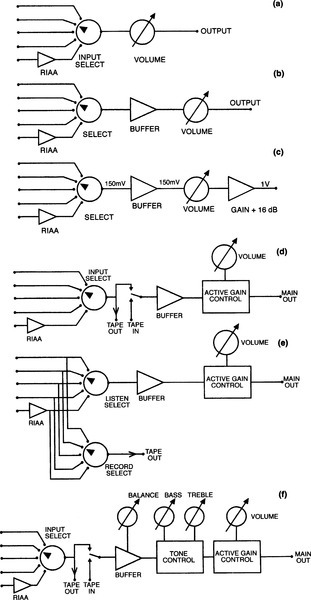
Minimal requirements are source selection and level control, as in Figure 1(a); an RIAA disc preamp stage is one input option. This sort of ‘passive preamplifier’ (a nice oxymoron) is only practical if the main music source is a low-impedance high-level output like CD.
The only parameter to decide is the resistance of the volume pot; it cannot be too high because the output impedance, which reaches a maximum of one quarter the track resistance at − 6 dB, will cause high-frequency roll-off with the cable capacitance. On the other hand, if the pot resistance is too low, the source equipment will be unduly loaded. If the source is valve equipment, which does not respond well to even moderate loading, the problem starts to look insoluble.
Adding a unity-gain buffer stage after the selector switch, Figure 1(b), means the volume control can be reduced to 10 kΩ, without loading the sources. This still gives a maximal output impedance of 2.5 kΩ, which allows you only 5.4 m of 300 pF/m cable before the response is 1.0 dB down at 20 kHz. For 0.1 dB down at 20 kHz, only 1.6 m is permissible.
The input RC filters found on so many power-amps as a gesture against transient intermodulation distortion add extra shunt capacitance ranging from 100 pF to 1000 pF, and can cause additional unwanted h.f. roll off.
Unfortunately only a CD source can fully drive a power amplifier. Output levels for tuners, phono amps and domestic tape machines are of the order of 150 mV rms, while power amplifiers rarely have sensitivities lower than 500 mV. Both output impedance and level problems are solved by adding a second amplifier stage as Figure 1(c), this time with gain. The output level can be increased and the output impedance kept down to 100 Ω or lower.
This amplifier stage introduces its own difficulties. Nominal output level must be at least 1 V r.m.s. (for 150 mV in) to drive most power amps, so a gain of 16.5 dB is needed. If you increase the full-gain output level to 2 V r.m.s., to be sure of driving exotica to its limits, this becomes 22.5 dB, amplifying the input noise of the gain stage at all volume settings. Noise performance thus deteriorates markedly at low volume levels – the ones most of us use most of the time.
One answer is to split the gain before and after the volume control, so that there is less gain amplifying the internal noise. This inevitably reduces headroom before the volume control. Another solution is double gain controls – an input-gain control to set the internal level appropriately, then an output volume control that requires no gain after it.
Input gain controls can be separate for each channel, doubling as a balance facility.3 However this makes operation rather awkward. No matter how attenuation and fixed amplification are arranged, there are going to be trade-offs on noise and headroom.
All compromise is avoided by an active gain stage, i.e. an amplifier stage whose gain is variable from near-zero to the required maximum. You get lower noise at gain settings below maximum, and the ability to generate a quasilogarithmic law from a linear pot. This gives excellent channel balance as it depends only on mechanical alignment.
Design philosophy
There is great freedom of design in small-signal circuitry, compared with the intractable problems of power amplification. Hence there is little excuse for a preamp that is not virtually transparent, with very low noise, crosstalk and THD.

Once all the performance imperatives are addressed, the extra degrees of freedom can be used to, say, make components the same value for ease of procurement. Opamp circuitry is used here, apart from the hybrid moving-coil stage. The great advantage is that all the tricky details of distortion-free amplification are confined within the small black carapace of a 5532.
One route to low noise is low-impedance design. By minimising circuit resistances the contribution of Johnson noise is reduced, and hopefully conditions set for best semiconductor noise performance. This notion is not exactly new – as some manufacturers would have you believe – but has been used explicitly in audio circuitry for at least 15 years.
In the equalisation and AGS stages, gains of much less than one are sometimes required. In these cases, avoiding the evils of attenuation-then-amplification (increased noise) and amplification-then-attenuation (reduced headroom) requires the use of a shunt feedback configuration. In the classic unity-gain stage, the shunt amplifier works at a noise gain of × 2, as opposed to unity, so using shunt feed-back introduces a noise compromise at a very fundamental level.
Absolute phase is preserved for all input and outputs.
The preamp gain structure
Compared with Ref. 1, the moving-magnet disc amplifier gain has been increased from + 26 to + 29 dB (all levels are at 1 kHz) to bring the line-out level up to 150 mV nominal. This is done to match equipment levels that appear to have reached some sort of consensus on this value. The input buffer has a gain of + 1.0 dB with balance central.
The maximum gain of the AGS is therefore reduced from + 26 to + 22 dB, to retain the same maximum output of 2 V. This affects only the upper part of the gain characteristic.
Disc input
While vinyl as a music-delivery medium is almost as obsolete as wax cylinders, there remain many sizable album collections that it is impractical to either replace with CDs or transfer to digital tape. Disc inputs must therefore remain part of the designer’s repertoire for the foreseeable future.
The disc stage here accepts a moving-coil cartridge input of 0.1 or 0.5 mV, or a moving-magnet input of 5 mV. It also includes a third-order subsonic filter and the capability to drive low impedances. The moving-coil stage simply provides flat gain, of either 10 or 50 times, while the moving-magnet stage performs the full RIAA equalisation for both modes.
Moving-coil input criteria
This stage was described in detail in Ref. 2. The prime requirement is a good noise figure from a very low source impedance – here 3.3 Ω to comply with, for example, the Ortofon MC10 cartridge. The circuit features
• triple low-rb input transistors
• two separate d.c. feedback loops
• combined feedback-network and output-attenuator.
The very low value of R6 means that a series capacitor to reduce the gain to unity at d.c. is impracticable; there is no d.c. feedback through R7, R10 around the global loop. Local d.c. negative feedback via R2, R3 sets input transistor conditions, and dc servo IC2 applies whatever is needed to IC1 non-inverting input to bring IC1 output to 0 V.
The two gains provided are 10 × and 50 ×, so inputs of 0.5 mV and 0.1 mV will give 5 m V r.m.s. out. The equivalent input noise of the moving-coil stage alone is − 141 dBu, with no RIAA. Johnson noise from a 3.3 Ω resistor is − 147 dBu, so the noise figure is a rather good 6 dB. Resistor R6 is also 3.3Ω. This component generates the same amount of noise as the source impedance, which only degrades the noise figure by 1.4 dB, rather than 3 dB, as transistor noise is significant.
If discrete transistors seem like too much trouble, remember a 5532 stage here would be at least 15 dB noisier.
The moving-magnet input stage
The first half of Morgan Jones’s excellent preamp article 5 appeared just after this preamp design was finalised. While I thoroughly endorse most of his conclusions on RIAA equalisation, we part company on two points. Firstly, I am sure that ‘all-in-one-go’ RIAA equalisation as in Figure 2(a) is definitely the best method, for IC op-amp designs at least. In my design the resultant loss of high-frequency headroom is only 0.5 dB at 20 kHz, which I think I can live with.
Secondly, I do not accept that the difficulties of driving feedback networks with low-impedance at h.f. are insoluble. I quite agree that ‘very few preamps of any age’ meet a + 28 dB ref 5 mV overload margin, but some exceptions are Ref. 1 with + 36 dB, Ref. 3 with + 39 dB, and Ref. 4 with a tour-de-force + 47 dB. My design here gives + 36 dB across most of the audio band, falling to + 33 dB at 20 kHz (due to h.f. pole-correction) and + 31 dB at 10 Hz (due to the IEC rolloff being done in the second stage).
Many contemporary disc inputs use an architecture that separates the high and low RIAA sections. Typically there is a low-frequency RIAA stage followed by a passive h.f. cut beginning at 2 kHz, Figure 2(b). The values shown give a correct RIAA curve.
Amplification followed by attenuation always implies a headroom bottleneck, and passive h.f. cut is no exception. Signals direct from disc have their highest amplitudes at high frequencies so this passive configuration gives poor h.f. headroom. Overload occurs at A1 output before passive h.f. cut can reduce the level.
Figure 3 shows how the level at A1 output (Trace B) is higher at h.f. than the output signal (Trace A). Trace C shows the difference, i.e. the head-room loss; from 1 dB at 1 kHz this rises to 14 dB at 10 kHz and continues to increase in the ultrasonic region. The passive circuit was driven from an inverse RIAA network. Using this, a totally accurate disc stage would give a straight line just below the + 30 dB mark.
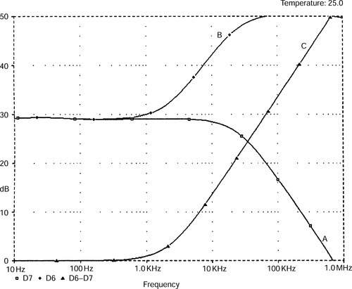
A related problem is that A1 in the passive version must handle a signal with much more h.f. content than A1 in Figure 2(a). This worsens any difficulties with slew-limiting and h.f. distortion. The passive version uses two amplifier stages rather than one, and more precision components.
Another difficulty is that A1 is more likely to run out of open-loop gain at h.f. This is because the response plateaus above 1 kHz, rather than being steadily reduced by increasing negative feedback. Passive RIAA is not an attractive option.
Alternatively there may be a flat input stage followed by a passive h.f. cut and then another stage to give the I.f. boost, which has even more head-room problems and uses yet more bits. The ‘all-in-one-go’ series feedback configuration in Figure 2(a) avoids unnecessary headroom restrictions and has the minimum number of stages.
In search of accurate RIAA
I have a deep suspicion that such popularity as passive RIAA has is due to the design being much easier. The time-constants are separate and non-interactive; only the simplest of calculations are required.
In contrast the series-feedback system in Figure 2(a) has serious interactions between its time-constants and design by calculation is complex. The values shown in Figure 2(a) are what you get if you ignore the interactions and simply implement the time-constants as Ra × Ca equals 3180 μs, Rb × Ca equals 318 μs, and Rb × Cb equals 75 μs. The resulting errors are ± 0.5 dB ref 1 kHz.
Empirical approaches (cut-and-try) are effective if great accuracy is not required, but attempting to reach even ± 0.2 dB by this route becomes very tedious and frustrating. Hence the Lipshitz equations6 have been converted to a spreadsheet, and used to synthesise the design in Figure 8.
A great deal of rubbish has been talked about RIAA equalisation and transient response, in perverse attempts to render the shunt RIAA configuration acceptable despite its crippling 14 dB noise disadvantage. The heart of the matter is that the RIAA replay characteristic apparently requires the h.f. gain to fall at a steady 6 dB/octave forever.
A series-feedback disc stage-with relatively low gain cannot make its gain fall below one, and so the 6 dB/octave fall tends to level out at unity early enough to cause errors in the audio band. Adding a high-frequency correction pole – i.e. low-pass time constant – just after the input stage makes the simulated and measured frequency response identical to a shunt-feedback version, and retains the noise advantage.
At this level of accuracy, the finite gain open-loop gain of even a 5534 at h.f. begins to be important, and the frequency of the h.f. pole is trimmed to allow for this.
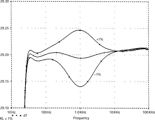
What RIAA accuracy is possible without spending a fortune on precision parts? The best tolerance readily available for resistors and capacitors is ± 1%, so at first it appears that anything better than ± 0.1 dB accuracy is impossible. Not so. The component-sensitivity plots in Figures 4, 5 show the effect of 1% deviations in the value of Ra, Rb; the response errors never exceed 0.05 dB, as there are always at least two components contributing to the RIAA response.

Sensitivity of the RIAA capacitors is shown in Figures 6, 7 and you can see that tighter tolerances are needed for Ca and Cb, than for Ra and Rb to produce the same 0.05 dB accuracy. The capacitors have more effect on the response than the resistors.
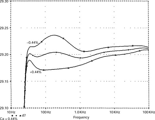

Finding affordable close-tolerance capacitors is not easy; the best solution seems to be, as in 1983, axial polystyrene, available at 1% tolerance. These only go up to 10 nF, so some parallelling is required, and indeed turns out to be highly desirable. The resistors are all 1%, which is no longer expensive or exotic, though anything more accurate certainly would be.
For Ca, the five 10 nF capacitors in parallel reduce the tolerance of the combination to 0.44%. This statistical trick works because the variance of equal summed components is the sum of the individual variances. Thus for five 10 nF capacitors, the standard deviation (square root of variance) increases only by the square root of five, while total capacitance has increased five times. This produces an otherwise unobtainable 0.44% close-tolerance 50 nF capacitor.
Similarly, Cb is mainly composed of three 4n7 components and its tolerance is improved by root-three, to 0.58%.
Noise considerations
The noise performance of any input stage is ultimately limited by Johnson noise from the input source resistance. The best possible equivalent input noise data for resistive sources, for example microphones with a 200 Ω source resistance, i.e. − 129.6 dBu, is well-known, but the same figures for moving-magnet inputs are not.
It is particularly difficult to calculate equivalent input noise for moving magnet stages as a highly inductive source is combined with the complications of RIAA equalisation.7 The amount by which a real amplifier falls short of the theoretical minimum equivalent input noise is the noise figure, NF. 1 often wonder why noise figures are used so little in audio; perhaps they are a bit too revealing.
The noise performance of disc input stages depends on the input source impedance, the cartridge inductance having the greatest influence. It is vital to realise that no value of resistive input loading will give realistic noise measurements.
A 1kΩ load models the resistive part of the cartridge impedance. But it ignores the fact that the ‘noiseless’ inductive reactance makes the impedance seen at the preamp input rise very strongly with frequency, so that at higher frequencies most of the input noise actually comes from the 47 kΩ loading resistance. I am grateful to Marcel van de Gevel8 for drawing my attention to this point.
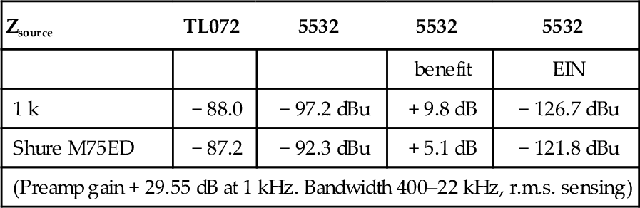
Hence, for the lowest noise you must design for a higher impedance than you might think, and it is fortunate that the RIAA provides a treble roll-off, or the noise problem would be even worse than it is. This is not why it was introduced. The real reason for pre-emphasis/de-emphasis was to discriminate against record surface noise. Table 1 shows the two most common audio op-amps, the 5532 being definitely the best and quieter by 5 dB.
Table 1
Measured noise results, showing the 5532’s superiority
| Zsource | TL072 | 5532 | 5532 | 5532 |
| benefit | EIN | |||
| 1 k | − 88.0 | − 97.2 dBu | + 9.8 dB | − 126.7 dBu |
| Shure M75ED | − 87.2 | − 92.3 dBu | + 5.1 dB | − 121.8 dBu |
| (Preamp gain + 29.55 dB at 1 kHz. Bandwidth 400–22 kHz, r.m.s. sensing) | ||||
To calculate appropriate EINs, I built a spreadsheet mathematical model of the cartridge input, called MAGNOISE. The basic method is as in Ref. 9. The audio band 50–22 kHz is divided into nine octaves, allowing RIAA equalisation to be applied, and the equivalent generators of voltage noise (en) and current noise (in) to be varied with frequency.
Noise generated by the 47 kΩ resistor Rin is modelled separately from its loading effects so its effect can be clearly seen. I switched off the bottom three octaves to make the results comparable with real cartridge measurements that require a 400 Hz high-pass filter to eliminate hum, and 1/f effects are therefore neglected. No psychoacoustic weighting was used, and cartridge parameters were set to 610 Ω+470 mH, the measured values for the Shure M75ED.
The results match well with my 5532 and TL072 measurements, and I think the model is a usable tool. Table 2 shows some interesting cases; output noise is calculated for gain of + 29.55 dB at 1 kHz, and signal-to-noise ratio for a 5 mV r.m.s. input at 1 kHz.
Table 2
Calculated minimum noise results
| Case | en | in | Rin | Ro(R) | Output | S/N ref (dB) | EIN |
| nV/√Hz | pA/√Hz | dBu | 5 mV | dBu | |||
| 1 Noiseless amp | 0 | 0 | 1000 M | 0 | − 104.0 | − 89.7 | − 133.5A |
| 5 Noiseless amp | 0 | 0 | 47 k | 0 | − 97.1 | − 82.8 | − 126.5C |
| 7 Noiseless amp | 0 | 0 | 47 k | 220 | − 96.7 | − 82.4 | − 126.2 |
| 11 2SB737, lc = 70 μA | 1.7 | 0.4 | 47 k | 220 | − 95.3 | − 81.0 | − 124.8 |
| 16 5532 | 5 | 0.7 | 47 k | 220 | − 92.5 | − 78.2 | − 122.0 |
| 18 TL072 | 18 | 0.01 | 47 k | 220 | − 86.9 | − 72.6 | − 116.5 |

I draw the following conclusions. The minimum equivalent input noise from this particular cartridge, without the extra thermal noise from the 47 kΩ input loading, is − 133.5 dBu, no less than 7 dB quieter than the loaded cartridge. (Case 1) It is the quietest possible condition. The noise difference between 10 MΩ and 1 MΩ loading is still 0.2 dB, but as loading resistance is increased further to 1000 MΩ the EIN asymptotes to − 133.5 dBu. A 47 kΩ loading is essential for correct cartridge response.
With 47 kΩ load, the minimum EIN from this cartridge is − 126.5 dBu. (Case 5) All other noise sources, including R0, are ignored. This is the appropriate noise reference for this preamp design.
Resistor R0, the 220 Ω resistor in the bottom arm of negative feedback network, adds little noise. The difference between Case 5 and Case 7 is only 0.3 dB.
A disc preamp stage using a good discrete bipolar device such as the remarkable 2SB737 transistor (rb only 2 Ω typ) is potentially 2.8 dB quieter than a 5532, when the noise from R0 and the input load are included. Compare Cases 11 and 16.
The calculated noise figure for a 5532 is 4.5 dB. Measured noise output of the moving magnet stage is − 92.3 dBu (1 kHz gain + 29.5 dB) and so the equivalent input noise is − 121.8 dBu, and the real noise figure is 4.7 dB, which is not too bad. Noise from the subsonic filter is negligible.
Taking en and in from data books, it looks as though the 5534/5532 is the best op-amp possible for this job. Other types – such as OP-27 – give slightly lower calculated noise, but measure slightly higher. This is probably due to extra noise generated by bias current-cancellation circuitry.8
There is an odd number of half-5532 s, so the single 5534 is placed in the moving-magnet stage, where its slightly lower noise is best used. The RIAA-equalised noise output from the disc stage in moving-coil mode is − 93.9 dBu for 10 × times gain, and − 85.8 dBu for 50 × times. In the 10 × case the moving-coil noise is actually 1.7 dB lower than movingmagnet mode.
Circuit details
The complete circuit of the disc amplifier and subsonic filter is Figure 8. Circuit operation is largely described above, but a few practical details are added here. Resistors R9 and R12 ensure stability of the moving-coil stage when faced with moving-magnet input capacitance C8, while R8 and R11 are dc drains.

The 5534 moving-magnet stage has a minimum gain of about 3 ×, so compensation should not be required; if it is, a position is provided (C26) for external capacitance to be added; 4.7 pF should be ample. The moving magnet stage feedback arm R20 −23 has almost exactly the same d.c. resistance as the input bias resistor R18, minimising the offset at the output of IC3. The h.f. correction pole is R24 + R25 and C20.
Capacitor C24 is deliberately oversized so low loads can be driven. Resistor R31 ensures stability into high-capacitance cables.