
Diagnosing distortions
This chapter focuses on the visual appearance of the distortion residuals produced by THD analysis. The distortion products may be low-order, in which case they appear simply as second or third harmonic, looking basically sinusoidal.
Crossover distortion, the greatest disturbance in the amplifier designer’s peace of mind, is instantly recognizable not only by its shape but by its timing, coinciding as it does with the zero-crossings of the output waveform. The other distortions are slightly harder to distinguish, as they all have their origin in contamination of the signal with half-wave rectified sinewaves, and so the different residuals look similar. Fortunately it usually takes only one or two simple experiments to determine the root cause of the trouble. On several occasions I have watched people trying to impose their will on a recalcitrant design without looking at the distortion residual, an approach which leaves me shaking my head in bafflement. To me the THD analyser is as much a part of the amplifier designer’s armoury as the doctor’s stethoscope, the pathologist’s microscope or even the geologist’s hammer.
In recent years, some audio commentators have been rudely dismissive of the simplest and most basic kind of distortion measurement – the total-harmonic distortion, or THD, test.
Because THD measurement has a long history, it is easy to imply that it is outdated and used only by the clueless. This is not so. Many other distortion tests exist, but none of them allows instant diagnosis of audio problems with one glance at an oscilloscope.
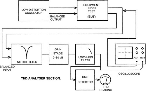
The test requires an oscillator with negligible distortion, feeding the unit under test. A notch-filter then completely suppresses the fundamental, to reveal the distortion products that have been generated. What remains after the fundamental is removed is not unnaturally called the THD residual.
In several previous articles I have described the various distortions that afflict audio power amplifiers. In the generic circuit, these are relatively few in number as is evident from the panel entitled ‘Distortion mechanisms’. Here I will show what some of these distortion residuals actually look like. Distortions 1, 2, 4 and 8 are not very informative visually, being essentially second or third harmonic, so I have omitted them to make room for the more complex waveforms specific to Class B.
Making distortion measurements
Total harmonic distortion is the r.m.s. sum of all the distortion components generated by the path under test. It is usually quoted as a percentage of the total signal level.
The r.m.s. calculation – taking the square-root of the sum of the squares of the harmonics – emphasises spiky distortions, but whether this helps to mimic human perception of distortion is unclear. The peak capability of true-r.m.s. circuitry is limited, and this may well lead to under-reading of crossover spikes and such.
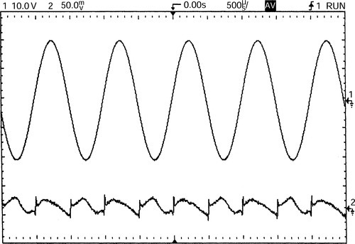
I hold that the best method is to observe the residual simultaneously, and time-aligned, with the output sinewave as in Figure 1. If you are testing similar pieces of equipment, then the gain of the oscilloscope’s second channel for the residual can be kept at the same setting. This allows linearity to be assessed at a glance.
In contrast, it is wiser to connect the actual output to channel 1, rather than an auto-scaled version from the analyser, as this prevents parasitics, etc., from being filtered out by the analyser input circuitry.
The beauty of THD testing is that the error is isolated; in essence, the residual is the difference between perfection and reality. When viewed time-aligned with the output sinewave, crossover distortion can be diagnosed immediately as it occurs at the zero-crossings. On the other hand, non-linearity confined to one peak is probably due to something running out of voltage swing or current capability.
Two technical challenges
Figure 1 shows the basic THD measuring system. There are two major technical challenges to be overcome. The signal source must be extremely pure, as any oscillator distortion puts an immediate limit on the measurement floor; it must maintain superb performance at least over the range 10 Hz to 20 kHz. A balanced output is highly desirable.
In the analyser section a balanced input is essential. Very great attenuation of the fundamental is required – about 120 dB if you are going to measure down to 0.0005%, making notch tuning is extremely critical. This cannot be attained by fixed-tuned filters, and manual tuning, requiring at least six controls, is about as much fun as picking oakum. In modern THD equipment both frequency and phase are continuously adjusted by a twin servo-loop that optimises the cancellation.
An additional low-pass filter defines the measurement bandwidth. Usually, 80 kHz is a good compromise, retaining most of the important harmonics while reducing noise. A switchable 400 Hz high-pass filter is often fitted, allowing measurements at 1 kHz and up, in the presence of hum. Such a filter should be used only in exceptional cases, for THD often rises sharply at low frequencies, and this would be missed.
While frequently advocated as a more searching examination of an audio path, twin-tone intermodulation tests are almost useless for circuit investigation. They give very little information about the source of the non-linearity as the phase relationship between the test signal and the result is lost. It is often claimed they give a better measure of audible degradation in real use, but a test using two or three tones is still a long way away from music that has tens or hundreds of simultaneous frequencies. Intermodulation tests can often dispense with very-low-THD oscillators, but this in itself is not much of a recommendation.
If real subjective degradation is the issue, a test signal much closer to reality is required. This can be either pseudorandom noise as in the Belcher test,1 or real music, as in the Baxandall2 and Hafler 3 cancellation tests.
Returning to harmonic distortion, much better correlation between THD measurements and subjective impairment is possible if the harmonics are weighted so that the higher order components are emphasised.
Weighting by n2/4, so that the second harmonic is unchanged, the third increased by 9/4, and so on, is generally accepted to be roughly correct.4,5 I was surprised to find that this approach goes back to 1937 and before.6 I doubt however whether this can be applied to crossover distortion.
When the THD residual is displayed on an analogue oscilloscope, artifacts in the noise are easily detectable by the averaging processes of our vision, but they remain unavailable to conventional measurement. A digital scope can perform even more effective averaging by computation, making submerged distortion artifacts both visually clearer and readily measurable, though an r.m.s. mode may not be available.
If a noisy signal is averaged two times, by combining two sweeps, the coherent signal stays at the same level, while the uncorrelated noise decreases by 3 dB. Averaging 64 times performs this process six-fold, so noise is then reduced by 18 dB. The oscilloscope used here was a digital HP54600B 100 MHz digital storage; an excellent instrument. This choice will not come as a surprise to alert readers.
Although sometimes invaluable, digital oscilloscopes are often not the best choice for audio THD testing and general amplifier work; in particular the problems of aliasing make the detection and cure of h.f. oscillations very difficult.
To create the residuals shown here, a Blameless amplifier was used essentially identical to that published in Ref. 7. Output was 25 W into 8 Ω, or 50 W into 4 Ω. The Blameless amplifier concept is outlined in a separate panel.
Crossover distortion
Crossover distortion is only one of the three components that make up Distortion 3 but is often the dominant one. Blameless amplifiers show only crossover distortion when driving 8 Ω or more, and at low and medium frequencies it should be below the noise. This remains true even if the amplifier noise is within a few decibels of the theoretical minimum from a 50 Ω source resistance.
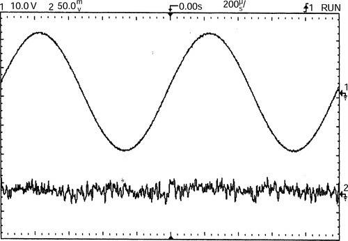
Figure 2 shows the THD residual from such a Blameless power amplifier, with optimally biased in Class-B. Since this is a record of a single sweep, the residual appears to be almost wholly noise. The visual averaging process is absent and so the crossover artifacts are actually less visible than on an analogue scope in real time.
In Figure 3, 64 times digital averaging is applied, which makes the disturbances around crossover very clear. A low-order component at roughly 0.0003% is also revealed, which is probably due to very small amounts of Distortion 6 that were not visible when the amplifier layout was optimised.
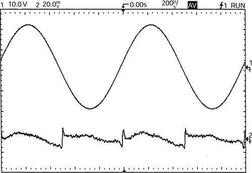
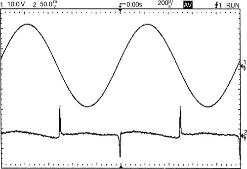
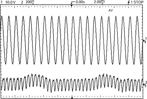
Figure 4 shows Class B mildly underbiased to generate crossover distortion. The crossover spikes are very sharp, and their height in the residual depends critically on measurement bandwidth. Their presence warns immediately of underbiasing and avoidable crossover distortion.
In Figure 5 an optimally-biased amplifier is tested at 10 kHz. The THD has increased to approx 0.004%, as the amount of global negative-feedback is 20 dB less than at 1 kHz. The crossover events appear wider than in Figure 3. The higher THD level is above the noise so the residual is averaged eight times only.

The measurement bandwidth is still 80 kHz, so harmonics above the eighth are lost. This is illustrated in Figure 6, which is Figure 5 rerun with a 500 kHz bandwidth. The distortion products look very different.

The 80 kHz cutoff point is something of de facto standard, which is reasonable as it seems highly unlikely that ultrasonic harmonics can detract from one’s listening pleasure. This does not mean THD testing can stop at 10 kHz, as there might be an area of bad intermodulation in the top octave.
My practice is to test up to 50 kHz, to check that nothing awful is lurking just outside the audio band; this is safe for moderate powers, and short durations.
Classes B and AB
I showed in my series on power amplifier distortion7 that Class AB is not a true compromise between Class A and Class B operation. If AB is used to trade off efficiency and linearity, its linearity is superior to B since below the AB transition level, it is pure Class A.
The Class-A region can – and should – have very low THD indeed, below 0.0006% up to 10 kHz, as demonstrated in Ref. 8. However, above the AB transition level THD abruptly worsens. This is due to what has been called ‘gm -doubling’, but is better regarded as a step in the gain/output-voltage relationship. Linearity is then inferior not only to Class-A but also to optimal-bias Class-B.
It is possible to make Class AB distortion very low by proper design. Basically, this means using the lowest possible emitter resistors to reduce the size of the gain step.9 Even so, THD remains at least twice as high as Class-B.
Tweaking up the bias of a Class-B amplifier most certainly does not offer a simple trade-off between power dissipation and overall linearity, despite the constant repetition this notion receives in some parts of the audio press. The real choice is: very low THD at low power and high THD at high power, or medium THD at all powers. The electricity bill is another issue.
Figure 7 shows the gain-step distortion introduced by Class AB. The undesirable edges are caused by gain changes that are no longer partially cancelled at the crossover; they are now displaced to either side of the zero-crossing. No averaging is used here as the THD is higher and well above the noise.

Large-signal non-linearity
When the load resistance falls below 8 Ω, extra low-order distortion components appear. This is true for most or all modern power bipolar junction transistors, but with old devices like 2 N3055, some large-signal nonlinearity may appear at 8 Ω. This is a compressive non-linearity, i.e. gain falls as level increases, ‘squashing’ the signal, and is due to fall-off of transistor beta at high collector currents.
Figure 8 shows the typical appearance of large-signal non-linearity, driving 50 W into 4 Ω, and averaged 64 times. The extra distortion appears to be a mixture of third harmonic, due to the basic symmetry of the output stage, with some second harmonic, because the beta-loss is component-dependant and not perfectly symmetrical in the two halves of the output.
Other distortions
Of the distortions that afflict generic Class-B power amplifiers, 5, 6 and 7 all look rather similar in the THD residual. This is perhaps not surprising since all result from adding half-wave disturbances to the signal.
Distortion 5 is usually easy to identify as it is accompanied by 100 Hz power-supply ripple; 6 and 7 introduce no ripple. Distortion 6 is easily identified if the d.c. power cables are movable, for altering their run will strongly affect the quantity generated.
Figure 9 shows Distortion 5, provoked by connecting the negative supply rail decoupling capacitor to the input ground instead of giving it its own return to the far side of the star point. Doing this increases THD from 0.00097% to 0.008%, mostly as second harmonic. Ripple contamination is significant and contributes to the THD figure. It could be easily filtered out to make the measurement, but this is just brushing the problem under the carpet.
Distortion 6 is displayed in Figure 10. The negative supply rail was run parallel to the negative-feedback line to produce this diagram. Although more than doubled, THD is still relatively low at 0.0021%, so 64-times averaging is used.

Figure 11 shows a case of Distortion 7, introduced by deliberately making a minor error in the negative feedback take-off point.

If it is attached to a part of the Class-B output stage so that half-wave currents flow through it, rather than being on the output line itself, THD is increased. Here it rose from 0.00097% to 0.0027%, caused by taking the negative feedback from the wrong end of the leg of one of the output emitter resistors, Re.
Note this was at the right end of the resistor, otherwise THD would have been gross, but 10 mm along a very thick resistor leg from the output line junction. Truly, God is in the details.
Diagnosis
The rogue’s gallery of real-life THD residuals portrayed here will hopefully help with the problem of identifying the distortion mechanism in a misbehaving amplifier. There is no reason why the generic/Lin configuration should give measurable THD at 1 kHz, or more than say, 0.004% at 10 kHz when driving 8 Ω.
It is important to be sure that you are measuring a real distortion mechanism, and not the results of parasitic oscillation upsetting circuit conditions; the oscillation itself may be outside the scope bandwidth. Parasitics usually vary greatly when a cautious finger is applied to the relevant section of the circuitry. Real distortion changes little, though the THD reading will probably be increased by the introduction of hum.
I hope I have shown that THD testing gives an immediate view into circuit operation that other methods do not, however useful they may be in other applications.
It cannot be stated too strongly that to attempt amplifier design and diagnosis without continuous visual observation of the THD residual is to work blind. You will proverbially fall into the ditch.