3

Slicing Things Like Pizzas and Watermelons

We Start with Pizza

Our problem begins with the supposition that you have a large pizza in front of you and you want to obtain the maximum number of pieces with a certain number of straight line slices. With one slice you get two pieces of pizza, two slices give you four pieces, and three slices get you six, right?

Not necessarily. If your third slice avoids the intersection of the first two slices, you will have a total of seven pieces.

A short pause while you get a pad of paper, a pencil, and a ruler. All set? Draw a straight line and then another that intersects the first. These are slices one and two and you have four pieces. Another line—slice three—gives seven pieces and slice four yields eleven. Slices five and six give sixteen and twenty-two, respectively.

By now it is getting to be a bit difficult to count the pieces. Never mind. We shall use what we now know. Let C be the number of slices or cuts and let P be the total number of pieces. Also let ΔP be the difference between successive values of P and let Δ²P be the difference of the difference. We compute these quantities, ΔP and Δ²P, to determine whether a clear mathematical pattern develops as the P sequence increases. Thus, we have the numbers shown in table 3.1.

TABLE 3.1

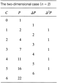
This is very interesting, especially the ΔP and the Δ²P columns. At this point, you probably discover what seems to be the rule to determine values of P for whatever value of C. The sequence of Δ²P is just a string of ones and the sequence of ΔP is simply ordinary counting. So, for C = 7 you predict P = 29 and for C = 8 you anticipate P = 37. You have indeed determined the sequence of P (viz., 1, 2, 4, 7, 11,…).

All right. A logical next question to ask is, how many pieces of pizza do you get when C = 100? My heavens! There must be a better way to spend your time than to run through the entire 100-step sequence. We need to be very clever.

Let us try the following. You will observe in the table that P increases faster than C but not as fast as C². Well, let's assume that a simple polynomial equation in C will help us determine the pattern of the P sequence. So we write

with the idea that we can determine the values of a₁, a₂, and a₃ with what is already known. So we “point match” at (C = 0, P = 1), (C = 1, P = 2), and (C = 2, P = 4). Substitution of these pairs of (C, P) values in equation (3.1) provides three equations containing the three unknowns a₁, a₂, and a₃. Some easy algebra gives a₁ = 1/2, a₂ = 1/2, and a₃ = 1. Accordingly, equation (3.1) becomes

The subscript 2 connotes the n = 2 case. If C = 10 then P = 56 and, in response to the question, if C = 100 then P = 5,051.

This problem is a portion of one of the 100 Great Problems of Elementary Mathematics presented in the delightful book by Dörrie (1965). It and its somewhat more complicated extension—which we shall examine in a moment—were posed and solved by Jakob Steiner (1796-1863), a German mathematician who is considered to be one of the greatest of the modern geometers.

The problem, as stated by Steiner, is What is the maximum number of parts into which a plane can be divided by C straight lines? The answer given by Steiner is equation (3.2). For reasons that become clear shortly, it is written in the form

The subscript 2 is attached to emphasize that our pizza is a plane and so we are dealing with n = 2 dimensions.

An additional point needs to be mentioned. Frequently, we can describe a particular sequence in terms of a recurrence relationship. For example, in a later chapter we shall see that the sequence of the famous Fibonacci numbers can be specified by such a recurrence equation.

It turns out that we can also express our slicing number sequence by a recurrence relationship. A simple geometrical model yields the expression

where P_c and P_c+1 are, respectively, the number of pieces after C and C + 1 slices. This result is easy to verify. Clearly, equation(3.3) gives the number of pieces after C slices; call this P_c. Next, we replace C in equation (3.3) with the quantity C + 1. This gives the number after C + 1 slices; that is, P_c+1. Subtracting P_c from P_c+1 gives the result of equation (3.4).

Backing Up to a Dot and a Licorice String

Two not very fierce problems are now quickly settled. The first is the n = 0 dimension case: a point or dot on a piece of paper. There is not much to do here since we do not slice dots. Accordingly, P₀ = 1.

The second is the n = 1 dimension case: a licorice string. If C = 0 then P = 1; if C = 1 then P = 2; if C = 2 then P = 3, and so on. So now we have the two equations

These expressions handle the n = 0 and n = 1 cases.

Now We Slice a Watermelon

With a close look at equations (3.3) and (3.5), perhaps we can see how a general solution is developing. But we need not be hasty. For the three-dimensional case (n = 3), we slice our watermelon once and so now we have two pieces, that is, C = 1, P = 2. Brilliant. Slice it again and we have C = 2, P = 4, and if C = 3 then P = 8. From here on, only those with unusually good spatial perception can deduce that if C = 4 then P = 15 and if C = 5 then P = 26.

Who needs spatial perception? Let mathematics do the work! We proceed with our analysis along two routes to obtain the solution we are after. We shall examine both of them.

Route 1

We construct a table similar to table 3.1 but extended to include the third differences, Δ³P. We start the construction of table 3.2 with the Δ³P column and, working from right to left, obtain the indicated P column sequence. This procedure is based simply on the conjecture that mathematics is logical and orderly. If that is the case, we now know that the n = 3 sequence follows the pattern 1, 2, 4, 8, 15, 26, 42, 64,…

TABLE 3.2

The three-dimensional case (n = 3)

Route 2

As we did in the n = 2 case with equation (3.1), we write

in which our polynomial in C commences with C³ instead of C². This time we point match with the first four (C, P) values shown in table 3.2. Substituting these into equation (3.6), we determine that a₁ = 1/6, a₂ = 0, a₃ = 5/6, and a₄ = 1. So the solution is

This is the answer provided by Dörrie (1965) to the problem presented by Steiner: What is the maximum number of parts into which a space can be divided by C planes?

Sure enough, the P values listed in table 3.2 agree with those computed from equation (3.7). Furthermore, for this n = 3 case, if C = 10 then P = 176 and if C = 100 then P = 166,751.

As before, we rewrite equation (3.7) in the form

Again, we can construct the recurrence relationship for this three-dimensional case (n = 3) in the same way we did for the two-dimensional case (n = 2) that led to equation (3.4). The answer is

Slicing Stuff in the Fourth and Higher Dimensions

Good gracious! It looks as if the general case solution is staring right at us. In equation (3.8), P₀ is the first term, P₁ is the first two terms, P₂ is the first three terms, and P₃ is all four terms. Logically, we next seek the answer for P₄, that is, n = 4. To exactly paraphrase and extend Steiner's question: What is the maximum number of parts into which a gizmo can be divided by C spaces?

A gizmo is a piece of something in four-dimensional space; better terminology is suggested, perhaps the word hypercube. However, this does not help much when we get to n = 5 and beyond. Some thoughts about “four-dimensional intuition” are presented by Davis and Hersh (1981). In any event, we should not let our inability to visualize further than n = 3 prevent us from proceeding with analysis. Going on to higher dimensions is certainly no problem as far as mathematics is concerned.

As before, there are the two routes to the solution. In the first route we construct a table similar to tables 3.1 and 3.2 but, this time, we include a Δ⁴P column; once again, this consists of the sequence of ones. Working from right to left we obtain the n = 4 sequence: 1, 2, 4, 8, 16, 31, 57, 99,…

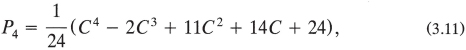
In the second route to the solution, we write down an equation, similar to equations (3.1) and (3.6). For this case, however, we surmise that we need to start with a C⁴ term. That is,

So now it is necessary to point match at five (C, P) values— (0, 1), (1, 2), (2, 4), (3, 8), (4, 16)—to determine the five coefficients; clearly, this will involve five simultaneous equations. The interesting book The Lore of Large Numbers, by Davis (1961), describes a procedure called the method of successive elimination to handle this kind of problem. An alternative approach is the method of determinants. Either methodology, with some algebra and arithmetic, provides the answer:

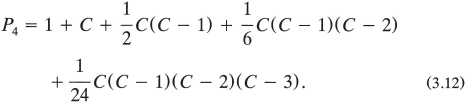
or, in the alternative form,

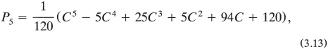
Similar methodology for the n = 5 case provides

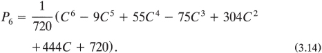
and for the n = 6 case,

From here on, it is not worthwhile to obtain solutions in this “power series” form, since now we believe we know how to express the answer for any value of n. That is, looking at equation (3.8) (for n = 3) and equation (3.12) (for n = 4), we write, for n = 5,

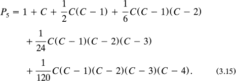
This seems to be the logical pattern for the P sequence. We surmise that the numbers appearing in the denominators of equation (3.15), that is, 1, 2, 6, 24, 120, are in fact the factorial numbers. That is, for example, 4!=4 × 3 × 2 × l = 24 and 5! = 5 × 4 × 3 × 2 × 1 = 120.

Now on to another matter. If you would like some good exercise in algebra, you can show that equation (3.15) reduces to equation (3.13) for the n = 5 case. Further, you can easily write down the equation for the n = 6 case in a form similar to equation (3.15). Then show that this expression reduces to equation (3.14).

Finally, it is reasonable to infer that the general solution to our problem is

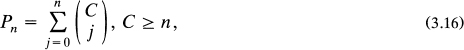
where is a symbol which indicates the summation of a series and

In addition, we have the special cases

For the limiting case in which C = n, Jolley (1961) gives

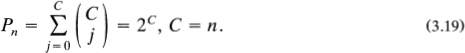
Expressions similar in form to equation (3.19) arise frequently in fields of mathematics called probability theory and combinatorics. In the vernacular of these fields, we would say that equation (3.17) gives the number of combinations of C things taken j at a time.

Some Examples of Slicing

So much for our analysis of the problem. Now for a few examples of applications.

EXAMPLE 1. A greedy land developer wants to know the maximum number of house lots he can obtain if he puts in 25 straight sidewalks across his large property. In this two-dimensional case (n = 2) we have from equation (3.16)

which becomes, using equation (3.17),

So, with C = 25, we determine that P = 326 lots. The same answer is provided, of course, by equation (3.2).

EXAMPLE 2. A weird architect wants to acquire the maximum number of rooms in a very large tall building he is designing. How many rooms can he get if 10 planes — defining rather strange walls, ceilings, and floors — are passed through the building? In this case, C = 10 and n = 3. Using equations (3.16) and (3.17), we obtain

Consequently, the architect can have 176 rooms of various shapes and sizes.

EXAMPLE 3. How many super-gizmos can we obtain from ten-dimensional space with 10 slices? Here, C = 10 and n = 10. Since C = n, we can use equation (3.19) to determine that P = 2¹⁰ = 1,024.

Linear Pattern Analysis in Geography

An important problem in geography and regional science has to do with the quantitative description of linear patterns in geographical settings. These patterns may represent roads and railroads, boundaries of cities and towns, river and stream networks, political districts, school zones, and other features of physical geography. Various techniques have been developed by researchers in these disciplines to analyze and classify these geographical patterns.

As described by Coffey (1981), one of the techniques to examine linear patterns was developed by Dacey, who utilized two-dimensional spacing as the basis of discrimination among patterns. He studied the three linear spacing patterns shown in figure 3.1.

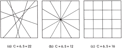
FIG. 3.1

Linear spacing patterns used in geographical analysis, (a) random, (b) radial, and (c) rectangular spacing.

Pattern 3.1(a) is essentially the n = 2 case we have been studying. This configuration is a random pattern of straight lines generated by connecting random points in a horizontal (x, y) plane. The equations of the array of lines are

where a_i and b_i are random values of slope and intercept.

If these quantities, a_i and b_i, are assigned designated values, then the random array of figure 3.1(a) reduces to the radial pattern of figure 3.1(b), at one extreme, and to the rectangular grid of figure 3.1(c), at the other. Detailed examinations of these geometries were carried out by Dacey; this enabled him to conduct so-called nearest-neighbor analyses. Such information is useful to geographers in studying things like marketing patterns, product distribution, traffic flow, settlement configuration, land utilization, and innovation diffusion.

We conclude with the observation that if figure 3.1 represents birthday cakes and if—for certain unspecified reasons—we are allowed exactly six slices, then obviously we get the most pieces of cake from figure 3.1(a). A bit messy and troublesome to serve perhaps, but still the most pieces.