
15
How Many People Have Ever Lived?
In 1990 the population of the world was approximately 5.32 billion people. This is an increase of 844 million over the 1980 population, which was an increase of 755 million over the 1970 population, which was an increase of 671 million over the 1960 population,…, and so on.
Interesting, but perhaps we are going the wrong way in time. Who cares about the population of the past—the demography of yesterday? We want to know about the population of the future—the shape of things to come. Two comments: First, the best way to make forecasts, at least for the near future, is to base projections on past and present information. Second, in the next chapter we shall indeed examine the topic of the world's population in the years to come.
So let us start by taking a look at the past. We begin with the following simple relationship:
![]()
in which N is the magnitude of a particular growing quantity at time t and a is a growth coefficient or an interest rate. This equation indicates that the rate at which a quantity is growing in magnitude is assumed to be directly proportional to the magnitude at that instant.
The solution to equation (15.1) is
![]()
where e, of course, is the base of natural logarithms and N0 is the magnitude of N at time t = 0. This is the equation for so-called exponential growth.
Without getting too complicated with our mathematics, (15.1) can be written in a more generalized form:
![]()
which is the same as (15.1) except that we have replaced a with the quantity a(N). This symbol says simply that the growth coefficient a is no longer constant but instead depends on the value of N. Let us be more specific about the form of a(N). We shall say that the growth coefficient or interest rate is directly proportional to N; that is, a(N) = aN/N0. This gives
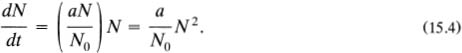
The quantity N0 is brought into the analysis at this point in order to keep the dimensions of the equation as simple as possible.
We note in (15.4) that the rate at which the particular quantity (e.g., population) is growing, dN/dt, is proportional not to the first power of N as in exponential growth, but to the second power, that is, the growth is like N squared. This kind of growth has been termed coalition growth by von Foerster et al. (1960).
As we shall see, coalition growth is truly “explosive” growth. It involves an increase to an infinite value of N in a finite time and it features a continuously shrinking “doubling time.” It incorporates, for example, the unbelievably good deal you got at your local financial house: your probably insane banker agrees to make your savings interest rate directly proportional to the amount you have on deposit (e.g., if you have $1000 in your account you get 4% interest; if you have $2000 you get 8%; $3000 gives 12%).
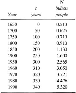
TABLE 15.1
Population of the world, 1650 to 1990
The solution to equation (15.4) is the amazingly simple expression
![]()
where N0 is the value of N when t = 0. This is the equation for coalition growth. Because of its mathematical form it is also called hyperbolic growth.
We go back to the population of the world. Information concerning the population is given in table 15.1 for the period from 1650 to 1990. We select 1650 as the year for which t = 0. The data shown in the table are plotted in figure 15.1. For the moment, disregard the solid curve shown in the figure.
It is observed that for a long time the world's population increased very slowly. Indeed, not until the beginning of the twentieth century did the population begin to rise sharply, and only after about 1950 did the population show really alarming increase.

FIG. 15.1
Population of the world, 1650 to 1990.
We suspect that this growth of population may have been more rapid than exponential growth. Hence, for starters, we assume it may be hyperbolic (or coalition) growth. To confirm this we need to see how the data “fit” the mathematical model. It is easy to rewrite equation (15.5) in the form
![]()
In the language of analytic geometry, this equation has the linear form ![]() where k0 and k1 are constants. Accordingly, if 1/N is plotted against t we should get a straight line if our assumption of hyperbolic growth is correct. The constants k0 and k1 provide the values of
where k0 and k1 are constants. Accordingly, if 1/N is plotted against t we should get a straight line if our assumption of hyperbolic growth is correct. The constants k0 and k1 provide the values of ![]() and a.
and a.
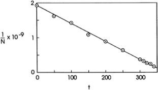
FIG. 15.2
Population of the world. Plot to determine numerical values of a and N0.
Such a plot is shown in figure 15.2. The fit of the data is remarkably good; the correlation coefficient is 0.9990. From a least squares analysis we obtain a = 0.002675 per year and ![]() Substitution of these numbers into equations (15.5) and (15.6) produces the solid lines shown in figures 15.1 and 15.2.
Substitution of these numbers into equations (15.5) and (15.6) produces the solid lines shown in figures 15.1 and 15.2.
Some questions: How many people were there in the world when Columbus discovered America? Taking t = 1492 – 1650 = –158 and substituting into (15.5) (with a = 0.002675 and N0 = 0.525 × 10⁹) gives N = 0.369 × 10⁹ or 369 million. How about that very eventful year 1066? Answer: 205 million. What was the world's population in the year 4000 B.C.? From equation (15.5) we get 33 million.
It is risky business to make population projections very far into the future based on some kind of formula or equation. It is equally risky to estimate or try to calculate past populations. Even so, our almost pitifully simple equation (15.5) gives answers about previous populations that agree amazingly well with values obtained by anthropologists and demographers using entirely different methodologies.
For example, Deevey (1960) estimates that the world's population was 125,000 a million years ago; equation (15.5) gives 196,000. Westing (1981) cites a population of 3,000,000 in the year 40,000 B.C.; we get 4,670,000. Austin and Brewer (1971) indicate a population of 100 million for the year 0 A.D.; we compute 97 million; and so on.
Our main question is: how many people have ever lived on earth? In 1990 the world's population was 5.32 billion. Is this a large or small percentage of the total number who have ever lived?
This question is answered by returning to equation (15.5). We integrate this equation to determine the total number of person-years, M, of all who have ever lived. That is,
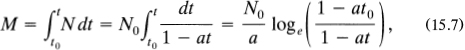
where we take t0 = –1,000,000 as the date from which we start counting the number of people who ever lived.
For example, how many people lived during the period t0 = –1,000,000 and t = –500,000? Substituting numbers into (15.7) gives M = 135.6 × 10⁹ person-years. Assuming a life span of duration ![]() yr gives
yr gives ![]() persons. In other words, about 5.4 billion people lived and died during the 500,000 years between 1,000,000 B.C. and 500,000 B.C.
persons. In other words, about 5.4 billion people lived and died during the 500,000 years between 1,000,000 B.C. and 500,000 B.C.
Some anthropologists and historians indicate that the year 4000 B.C. marks the “dawn of civilization.” If so, how many people lived in the predawn period, 1,000,000 B.C. to 4000 B.C.? From (15.7) we determine M = 1,003 × 109 person-years for that period and, with ![]() yr as the average life span, obtain P = 40.1 billion people.
yr as the average life span, obtain P = 40.1 billion people.
A listing of the cumulative number of people who have ever lived, commencing with the year 1,000,000 B.C., is shown in table 15.2. To follow the scheme of other studies of the subject, the average life span is taken as ![]() yr.
yr.
As they say, the bottom line is the answer. The last entry of table 15.2 indicates that through the year 1990, about 80 billion people have lived on earth. Some observations:
The world's population in 1990 was 5.32 billion. This is about 6.5% of the number of people who have ever lived. Said another way, about one person of fifteen who have ever lived is currently living.
TABLE 15.2
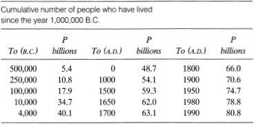
About half of the 80 billion people lived between 1,000,000 B.C. and 4000 B.C.; the other half since then.
During the nearly 2,000-year period from the year 0 A.D. to 1990, about 32 billion people have lived. This is 40% of the total who have ever lived.
Our final answer, P = 80 billion, agrees fairly well with results obtained by others; they range from 50 billion to 110 billion. Suggested references are Deevey (1960), Goldberg (1983), Keyfitz (1966), and Westing (1981).
We conclude our chapter with a word about the doubling time. By definition, this is simply the time required for a growing quantity to double in magnitude. For example, a quantity may be following an exponential growth relationship. If so, from equation (15.2) it is easy to establish that the doubling time, t2 is
![]()
For example, if the population growth rate of a certain country is a = 3.5% per year, then the doubling time is 20 years. This type of exponential population growth is sometimes called Malthusian growth. We note that one of the features of such growth is a constant doubling time.
In contrast, suppose that a quantity is growing according to a hyperbolic growth relationship. From equation (15.5) we obtain the following expression for the doubling time:
![]()
In this case, the doubling time, t2, is not constant, as in exponential growth, but instead changes with time. In the year 1000 A.D., for example, t = 1000 – 1650 = –650, and so, from equation (15.9), the doubling time t2 = 512 yr. In 1650, t2 = 187 yr; in 1950, t2 = 37 yr; in 1990, t2 = 17 yr.
This is getting to be rather scary. Does this mean that in the year 1990 + 17 = 2007, there will be 2 × 5.52 = 10.64 billion people in the world? And then it doubles again nine years after that? We shall examine these alarming questions in our next chapter, “The Great Explosion of 2023.”