22

Cartography: How to Flatten Spheres

It is said that Columbus must surely have been an economist, a stockbroker, or something like that to have successfully raised the funds for the journey of his three small ships across the Atlantic back in 1492. But even though Columbus did receive fairly strong financial support from the Spanish crown, he definitely was not an economist. In fact, he was a very competent seaman and, more importantly, he possessed considerable knowledge of and experience in the principles of navigation and geography.

The fact that Columbus mistook the vast land mass we now call the Americas for south or east Asia was not entirely his fault. By the late fifteenth century, when he made his journeys, there were quite accurate maps of most of Europe and the Middle East and fairly good maps of much of Africa and Asia. However, the New World simply did not exist!

Indeed, much of the geography of the Old World had been known since the time of the great astronomer Claudius Ptolemy of Alexandria (87–150). Even before that, the Babylonians, Persians, and Egyptians had produced maps of the then-known world and maps of the skies. By the fifth century, the Greeks had laid the foundations of what we now call cartography: the science and art of maps.

Over the centuries, a great many people made contributions to the development of maps and globes of the world and the heavens. Two names especially stand out in the long history of cartography. One is Ptolemy and the other is Gerhard Kremer (1512–1594); we know him better by his latinized name, Gerardus Mercator. Though born in Holland, he spent nearly all of his long life in Germany. In 1569 his famous Great World Map was published. Mercator's map, or more precisely, the Mercator projection of the world, is familiar to all of us; we shall return to it shortly.

There are numerous books devoted to the history of maps and cartography; those of Bagrow (1985) and Brown (1949) are recommended. Maps of the Heavens is the title of a beautiful book by Snyder (1984) dealing with cartography of the skies.

How Map Projections Are Classified

Suppose we have a globe or some other spherical object on which we have a map of the world, or indeed any kind of configuration or pattern of lines. Suppose also that we want to transform this three-dimensional sphere to a two-dimensional plane in order to produce a map of the world or pattern of lines on a nice sheet of flat paper.

Basically there are two methods to accomplish this. The first method is to place the sphere—the globe—under a powerful hydraulic press, like those used in steel mills, and flatten the heck out of it. We discard this procedure because it is not scientific. The second method is to utilize various techniques to transform the sphere mathematically onto a plane.

It turns out that it is impossible to transform a sphere to a plane without some kind of distortion in the map you are making. If you want to retain some features of the map in the transformation from sphere to plane (e.g., angles or distances), then you must sacrifice other features (e.g., areas or directions).

There are three types of surfaces we can use to transform or project a three-dimensional sphere onto a two-dimensional plane. These are illustrated in figure 22.1. The first is a plane surface itself; this is called the azimuthal projection. The second is the conical projection. In this case, after the sphere's pattern is projected onto the cone, a cut is made along the side of the cone and the surface is spread out to provide a flat map. The third is the cylindrical projection. Again, after the globe's pattern is projected, the cylinder is cut and laid flat.

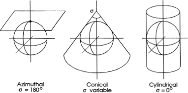
FIG. 22.1

Basic types of map projections.

As shown in the figure, these three basic geometries, the plane, cone, and cylinder, are tangent to the sphere at a certain point or along a certain curve. However, each of the three surfaces could actually intersect the sphere at a specified place; these are called secant projections. Although there are many applications for secant maps, we shall not consider them here.

From the preceding, we note that the first way to classify map projections is according to the type of plane surface onto which the sphere is projected: azimuthal, conical, or cylindrical.

A second way to classify projections is according to the projection source. For example, suppose we want to construct an azimuthal projection. That is, as shown in figure 22.2, we want to project point P of the sphere onto the plane. We could select the center of the sphere, point A, as the projection source and obtain point P₁ on the plane. This is called a gnomonic projection. Alternatively, the projection source could be at point B, located directly opposite the point of tangency T. This is called the stereographic projection; it produces point P₂ on the plane. Finally, we could move the projection source all the way to infinity at point C to generate point P₃ on the map. This is the orthographic projection.

FIG. 22.2

Types of projection sources, (a) APP₁. gnomonic. (b) BPP₂: stereographic. (c) CPP₃: orthographic.

There is a third way by which map projections can be classified. This classification specifies which properties we want to preserve as we transform from a sphere to a plane. There are four such properties:

Equal angles. This property, usually called the conformality property, assures that any angle on the sphere is transformed without change onto the plane. For example, the meridians (lines of constant longitude) and the parallels (lines of constant latitude), which are perpendicular on the sphere, are also perpendicular on the plane.

Equal areas. This property stipulates that every small region on the sphere has the same area after it is transformed onto the plane.

Equal distances. This property requires that distances from the center of a map projection be the same on the sphere and the plane.

True directions. This property means that directions from the center of a map projection must be identical on the surface and the plane.

As indicated above, it is not possible to preserve all these properties in a particular transformation. There must be tradeoffs. For example, the flag of the United Nations displays an azimuthal stereographic conformal (equal-angle) projection of the world with the point of tangency at the North Pole. The other properties are not preserved on this projection. Table 22.1 gives a summary of the various ways by which map projections are classified.

 

TABLE 22.1

Over the past two thousand years or so, many hundreds of different kinds of map projections have been devised. Of this very large number, perhaps fifty kinds find some type of present-day application and maybe a dozen or so can be described as extremely useful. Not surprisingly, mankind's relatively recent ventures into space exploration have produced renewed interest and great progress in mapping not only the earth but also the moon and nearby planets.

We are going to take a close look at only two of the many different kinds of projections. If you want to study cartography and map projection in detail, numerous books are available; some of the best are those of Raisz (1962), Snyder (1987), Snyder and Voxland (1989), and Snyder (1993).

In your studies, it will be very helpful if you know something about spherical trigonometry and solid analytic geometry. If you would like to become knowledgeable in cartography, you should study calculus and differential equations and also an interesting branch of mathematics called differential geometry.

The two projections we are going to examine in some detail are the Mercator projection and the Lambert azimuthal equal-area projection. We start with the first of these.

The Mercator Projection and Loxodromes

This projection was devised by the great Flemish cartographer Gerardus Mercator (1512–1594) and first appeared in 1569. It is developed onto a cylinder in such a way that angles are preserved (i.e., it is conformal). Without doubt, this is the most famous of all map projections. It has the great advantage that paths on a sphere that hold constant angle to the meridians (lines of constant longitude) transform onto a plane as straight lines. This feature is extremely useful in navigation. However, the Mercator projection has the great disadvantage that regions at high latitudes (at, say, 50° or more) are considerably enlarged and distorted. Indeed, the poles are infinitely large in area.

We begin our studies involving the Mercator projection with a geometrical analysis of a small area on the surface of a sphere. The following mathematical relationships are obtained:

where λ is the longitude, ø is the latitude, and θ is the angle that a certain path makes with a meridian. An incremental distance along the path is ds and R is the radius of the earth.

We rewrite the first of equations (22.1) in the form

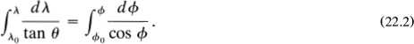
The lower limits on the integrals indicate that when λ = λ₀, ø = ø₀. If we assume that θ is constant, that is, the path is always at the same angle with the meridians, then (22.2) can be integrated to give

where the angles are expressed in radians. This equation is called the rhumb line or loxodrome. It transforms a straight line on the plane of a Mercator projection to a curved path on a sphere.

The second of equations (22.1) provides the expression

This simple equation gives the length S of the loxodrome between the point located at (λ₀, ø₀) and any other point (λ, ø).

In a moment, we return to our analysis of the Mercator projection and the Lambert azimuthal equal-area projection. But first, we need to take a close look at the following very remarkable phenomenon.

The Strange Behavior of the Mysterious Honking Bird

This is an appropriate place to describe and analyze the unbelievably strange behavior of the fascinating (and mythical) “honking bird.” This extremely interesting winged creature is hatched on or very near the earth's equator. Then, when it reaches a certain age, it mysteriously begins an east-northeastward migration, which ultimately terminates at the North Pole, although a small fraction of these birds prefer to fly to the South Pole. Whether heading toward the north or the south, the honking bird nevertheless flies on a path that always holds a constant bearing with the meridians. Typically, the bearing angle θ is around 80°.

At this point we pause to let our mathematics catch up with us. To simplify our equation, we let ø₀ = 0 in (22.3). Then we solve for ø to obtain

This expression provides the value of ø (latitude) for any value of λ (longitude).

In addition, from (22.4), we have, with ø₀ = 0,

This expression gives the total length of the loxodrome, S, between the equator and any latitude ø.

Back to our honking bird: We select the value θ = 80° as the bird's “true heading” from north. The source of its flight is on the equator (ø₀ = 0) near its well-known (but mythical) breeding ground along the northeastern shore of Lake Victoria in Africa (λ₀ = 35°E).

Remembering that ø and λ must be expressed in radians, we use equation (22.5) to compute the bird's position, ø = ƒ(λ).

At this point it is suggested that you get your globe and world atlas. It will be helpful if you have them for the following analysis. With θ = 80°, our honking bird is flying in an east-northeast direction. Hence, from (22.5), with λ₀ = 35°E, you easily calculate that when the bird is at longitude λ = 125°E (i.e., one-quarter of the way around the world), it is at latitude ø = 16°N. Your globe indicates that this location is east of the island of Luzon in the Philippines. Likewise, when the bird is at λ = 215°E (i.e., 145°W; halfway around the earth), then ø = 30°N; this is northeast of Hawaii.

After one complete trip around the world, our honking bird is at latitude ø = 53°N (near Moscow) and after two complete revolutions, it is at latitude ø = 78°N (west of Franz Joseph Land in the Arctic Ocean).

A sketch of the bird's loxodromic path is shown in figure 22.3. We note that the radius of its path, measured from the earth's axis, continuously decreases as it moves northward. Indeed, when the bird gets extremely close to the North Pole, the radius of its path begins to approach zero. At this point, this otherwise entirely silent bird emits a very loud honking noise, which is a signal to himself to get out of the way. Because of this strange behavior—the bird's once-in-a-lifetime brief but extremely loud traffic blast—ornithologists have logically dubbed it the honking bird.

How far did our feathered friend go on his journey from Lake Victoria to the North Pole? With ø = π/2 (i.e., 90°) in equation (22.6), we obtain

With θ = 80° and R = 6,370 km, we compute that S = 57,620 km or about 35,810 miles.

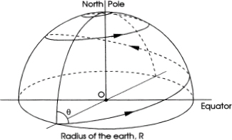
FIG. 22.3

The flight of the amazing honking bird.

The Mercator Projection Revisited

As shown in figure 22.1, the Mercator projection is constructed by wrapping a circular cylinder around the earth and tangent at the equator. If a tiny light source were at the center of a transparent globe, it would cast an image of the earth's land masses onto the cylinder. True enough, but this does not yield the Mercator projection; it might be called a gnomonic projection onto a cylinder. This projection is useless because there is extremely great distortion at high latitudes.

The Mercator projection is a conformal (i.e., angle-preserving) projection. From equation (22.1), the angle of an arbitrary path on a spherical surface is tan . It is not hard to show that on a cylindrical surface, the angle of the path is tan , where y is the distance measured in the direction of the cylinder axis. Requiring that θ = θ_* (i.e., equal-angle transformation), we obtain . In addition, we take where x is the distance measured along the equator. Integrating these expressions for dx and dy gives

These equations describe the positions of the meridians (lines of constant λ) and the parallels (lines of constant ø) on the projection. Clearly, on a Mercator map, the x-coordinate (east-west) is directly proportional to the longitude λ. However, the y-coordinate (north-south) is stretched increasingly as the latitude ø increases. When ø = π/2, y = ∞.

Here are some examples involving the Mercator projection.

Part I

A jet aircraft flies from New York to Tokyo along the great circle route. How far is its journey? Show its path on a Mercator map.

From our atlas we obtain the following information: New York, longitude λ₁ = 74°W, latitude ø₁ = 41°N; Tokyo, longitude λ₂ = 140°E, latitude ø₂ = 36°N. The law of cosines for a spherical triangle gives the equation

The values of λ and ø indicated above are substituted into this expression to calculate cos a. From this we obtain a = 97°, which is the angle of the great circle, measured at the earth's center, between New York and Tokyo. The distance S between the two cities is S = (a/360)2πR and, with R = 6,370 km, we obtain S = 10,785 km or about 6,700 miles.

The path of the jetliner's flight is shown as curve A on the Mercator map of figure 22.4. After leaving New York, the airliner proceeds along the western shore of Hudson Bay and then across northern Canada. It reaches a maximum latitude of 70°N at a longitude of 146°W. This is close to Prudhoe Bay on the Arctic shore of Alaska—the hub of the North Slope's vast petroleum fields. The flight then passes well north of the Bering Strait, flies through northeastern Siberia, along the Kamchatka Peninsula, and on to Tokyo.

FIG. 22.4

Mercator map with (curve A) the great circle and (curve B) the loxodrome between New York and Tokyo.

Part II

On its return journey, our jet airplane flies from Tokyo to New York along the loxodrome route. Again, how far is its flight? Show its path on a Mercator map.

The values of λ and ø for New York and Tokyo are substituted into equation (22.3) to determine that the constant true heading of the jet's loxodrome path is θ = 87.5°. Substituting back into (22.3) then provides the value of the longitude λ for any value of the latitude ø. This path is shown on curve B on the Mercator map of figure 22.4. This time our journey takes us across the wide expanse of the Pacific Ocean and over northern California, Denver, and Indianapolis, and then we land in New York.

From equation (22.4) we compute that the total length of our loxodromic flight is S = 12,745 km; this is about 18% longer than the great-circle flight.

The Lambert Azimuthal Equal-Area Projection

Another famous person involved in the development of cartography was the Swiss-German mathematician Johann Heinrich Lambert (1728–1777). Although he made contributions in many areas of mathematics, he will probably be best remembered for his work in cartography.

Perhaps his most noteworthy effort was what we now call the Lambert azimuthal equal-area projection, which he presented in 1772. This projection is employed extensively for maps of the polar regions.

We utilize this projection in figure 22.5 to display the northern hemisphere. The figure also shows the computed path of our jetliner flying from New York to Tokyo along the great circle (curve A) and also its route from Tokyo to New York along the loxodrome (curve B). Although this projection does not show true distances, it does indicate that the great circle is shorter than the loxodrome.

As the name implies, the Lambert azimuthal equal-area projection preserves areas. For example, the area of the island of Cuba (can you find it in figure 22.5? λ = 80°W, ø = 22°N) is the same on the plane map as it is on a spherical globe. The undesirable but necessary distortion requires that Cuba be stretched in the east-west direction and shrunk in the north-south.

The Berghaus Star Projection

As mentioned, over the years a great many kinds of map projections have been developed. We conclude our introduction to cartography with an example involving a rather artistic map projection: the Berghaus star projection.

FIG. 22.5

Lambert azimuthal equal-area map with (curve A) the great circle and (curve B) the loxodrome between New York and Tokyo.

This projection was devised in 1879 by the German cartographer Heinrich Berghaus (1798–1884). It is shown in figure 22.6. In this map, the northern hemisphere is an azimuthal equidistant projection. The southern hemisphere consists of five triangular lobes. As Snyder and Voxland (1989) indicate, this projection is used mainly for artistic forms.

In chapter 2, we carry out an extensive analysis of the dimensions and geometrical features of five-pointed stars. Included in that analysis is the special case that appears in the Berghaus star projection.

One of the features of the Berghaus star is that its radius is twice the radius of the circle containing the northern hemisphere. This is the region defined by the equator passing through the five longitude locations shown in figure 22.6. From our earlier analysis, the internal angle at the points is α = 52.53°.

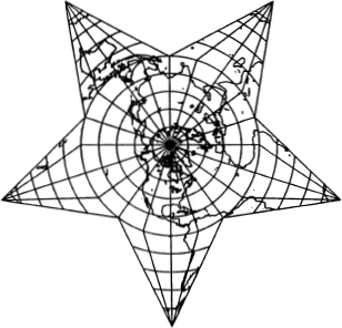
FIG. 22.6

The Berghaus star projection. (From Snyder and Voxland 1989.)

This is the shape of star that appears, or has appeared in the past, on the flags of various nations, including the flag of Vietnam during the period following World War II. It is interesting to note this rare linkage between vexillology (the science of flags) and cartography (the science of maps).

Looking Ahead in Cartography

Cartography is one of mankind's oldest sciences. It has been around as long as humans have navigated from here to there and as long as people have studied the skies. The science of cartography has evolved, slowly but steadily, over twenty-five to thirty centuries. During that very long period, many of the greatest mathematicians, astronomers, geographers, and navigators have contributed to the development of cartography and the making of maps.

In recent times—starting around 1950 or so—there have been many spectacular advances that have stimulated our interest in cartography and provided new methodologies to accelerate its further development. Incredible advances in space technology have given us extremely useful techniques for mapping not only the earth but also our celestial neighbors. Similar fantastic advances in computer technology have provided extremely rapid ways to analyze data, solve difficult mathematical problems, and graphically display all kinds of information.