9
Great Number Sequences: Prime, Fibonacci, and Hailstone
What Are Number Sequences?
The answer to this question is that number sequences are simply lists of numbers appearing in a particular order. For example, the sequence 0, 1, 2, 3, 4, 5, 6, 7, 8, 9 is the list of the natural numbers or integers. The sequence 1, 3, 5, 7, 9, 11 is the list of the odd integers and the sequence 1, 4, 9, 16, 25, 36 is the list of the squares of the integers.
Another example: The sequence 1, 2, 4, 8, 16, 32, 64 is the list of numbers generated by doubling successive numbers. Sometimes, as in this case, a mathematical formula can produce the sequence of numbers. In this example, the formula is N = 2n, where N is the magnitude of the nth number of the sequence. This particular sequence is the one that describes geometric growth; it is closely related to so-called exponential growth. This sequence is quite famous. In a quantitative way, it reflects the gloomy prediction of Thomas Malthus, the eighteenth-century English clergyman-economist, regarding the explosive growth of human population.
Here is an interesting sequence: 6, 28, 496, 8,128, and so on. This is the sequence of so-called perfect numbers. A perfect number is a number composed of the sum of all its divisors except the number itself. For example, it is clear that 6 and 28 are perfect numbers because 6 = 1 + 2 + 3 and 28 = 1 + 2 + 4 + 7 + 14.
These numbers were known and studied by the Greeks more than two thousand years ago. An interesting fact is that the next perfect number in the sequence, following the 8,128, is 33,550,336. After that come 8,589,869,056 and then 137,438,691,328. At present (1999), we know the values of thirty-six perfect numbers. In recent years, the rapid development of computers has accelerated our search for these numbers.
There are a great many sequences in mathematics; some are important or interesting, others are trivial or silly. Over the years, a very large number of sequences have been discovered or devised. A collection of over 2,300 from all branches of science and mathematics has been nicely assembled by Sloane (1973). On the following pages, we shall investigate a few.
Mostly about Prime Numbers
Suppose we have the following sequence of positive numbers: 1, 2, 3, 5, 7, 11, 13, 17, 19, 23, 29, 31, 37, and so on. Does this sequence represent anything in particular?
It certainly does. It is the sequence of so-called prime numbers. That is, it is a list of the numbers that are exactly divisible only by 1 and the number itself. For example, 13 is a prime number because it can be exactly divided only by 1 and 13. On the other hand, 12 is not a prime number; in addition to 1 and 12, it can also be divided by 2, 3, 4, and 6.
The natural numbers or integers are 1, 2, 3, 4, 5, 6, 7, 8, and so on. If a natural number is neither 1 nor a prime it is called a composite number. Following the 37, the above sequence of prime numbers continues: 41, 43, 47, 53, 59, 61, 67, and so on. Altogether, there are 168 prime numbers less than 1,000 and, with the exception of 2, they are all, of course, odd numbers. By the way, mathematicians usually do not consider 1 to be a prime number.
It turns out that the sequence of prime numbers goes on forever. The famous Greek geometer Euclid was the first to prove this; the year, around 300 B.C. Ever since then, mathematicians have been trying to discover or develop a method or an equation to determine whether or not a particular number is a prime number. So far, they have not been successful.
Long ago, numerous formulas were devised that generated prime numbers. A good example is the expression N = n2 – 79n + 1601. This formula produces prime numbers for all values of n up to and including n = 79. You might want to check a few. However, when n = 80, the formula fails because N = 1681 = 41 × 41. Thus, 1681 is a composite number. Other early expressions for generating prime numbers were N = n2 – n + 41 and N = n2 + n + 17. With the benefit of hindsight, it now seems obvious that these polynomial-type expressions are entirely inadequate in producing a lengthy list of only prime numbers.
The noted French mathematician Pierre de Fermat (1601-1665) also searched for a formula that would yield only prime numbers. He invented the following equation, which produces what we now call the Fermat numbers:
![]()
This expression generates the numbers F0 = 3, F1 = 5, F2 = 17, F3 = 257, and F4 = 65,537. All of these numbers are prime. However, F5—which is a ten-digit number—is not prime and neither are the Fermat numbers corresponding to n = 6, 7, 8, 9, 11, and many more numbers calculated with larger values of n. So Fermat was mistaken about equation (9.1) producing only prime numbers. Indeed, a present-day question in number theory is, are any Fermat numbers, larger than n = 4, prime numbers? So far, the question has not been answered.
Mathematicians have long since abandoned the search for formulas that generate prime numbers; there are a great many more interesting subjects in number theory for them to investigate. The following is an important example.
How Are the Prime Numbers Distributed?
It is well known that the sequence of prime numbers goes on forever. However, as the numbers become larger and larger, their frequency decreases, that is, the gaps between successive primes increase. This feature provided the historical basis for the statement of the fundamental theorem of prime numbers. This theorem, for which there are now numerous proofs, postulates that as n increases to very large values, the number of primes not exceeding n is given by the expression
![]()
The problem attracted the attention of many of the leading mathematicians of the past. The German mathematician Carl Friedrich Gauss (1777-1855), one of the greatest of all time, examined the problem of prime number distribution in 1792 when he was only fifteen years of age.
Table 9.1 may help illustrate our point concerning the distribution of primes. In the table, column 2 indicates that there are 168 prime numbers less than 1,000. Column 3 says that the number of primes, computed from equation (9.2), is 145, which is somewhat less than the actual number. As shown in column 4, the ratio of column 3 to column 2 is 0.863.
TABLE 9.1

Source: Lines (1986).
Now observe that as the number n increases, the ratio of the two quantities of prime numbers, shown in column 4 of the table, gradually increases and appears to approach the limiting value 1.0. Indeed, if n = 1 billion the ratio is 0.949 and if n = 10 billion the ratio is 0.954. This is precisely the result postulated by the prime number theorem.
The entire matter can be carried a significant step further. Studies have shown that an even more accurate answer to the prime number theorem is given by the expression
![]()
where Li(n) is the so-called logarithmic integral. The indicated integral is tabulated in numerous mathematical handbooks.
For the sake of completeness, the number of primes determined by equation (9.3) is listed in column 5 of table 9.1. If these numbers are compared with those shown in column 2 of the table, we note very close agreement. Thus, the accuracy of equation (9.3) in predicting the distribution of prime numbers is quite remarkable.
What Is the Largest Prime Number?
Of course, one of the greatest challenges to mathematicians is to discover ever-larger prime numbers. Over the years, the magnitude of the largest known prime number has steadily increased; clearly, the very rapid advances in computer technology have greatly assisted these efforts. Currently (1999), the largest known prime number is 23,021,377 – 1. This number is so enormous that it requires 909,526 digits to express it.
Not surprisingly, some of the greatest mathematicians of all time have worked on the theory of prime numbers. If you are interested in the historical aspects of the subject, Bell (1956) and Boyer (1991) are good places to start. Elementary presentations of topics on prime numbers are given by Beiler (1964), Lines (1986), and Ogilvy and Anderson (1988). A more advanced coverage is presented in the very readable book by Ribenboim (1995), which includes a lengthy list of references.
Concerning Fibonacci Numbers
One of the most remarkable sequences of numbers in mathematics is the Fibonacci sequence or simply the Fibonacci numbers.
The story all began about eight hundred years ago when an Italian mathematician named Leonardo of Pisa (1170–1250)—better known as Fibonacci—wrote a book entitled Liber Abaci (first published in 1202; revised in 1228). He was born in Pisa, Italy, at about the time construction was begun on what is now called the Leaning Tower of Pisa (which was completed around 1300). Incidentally, he lived long before Galileo Galilei (1564–1642) carried out his famous weight-dropping experiments from the top of the tower.
During much of his early life, Fibonacci lived in North Africa and studied algebra and geometry under Arabic mathematics teachers. As a result, he learned a great deal about the Arabic number system and decimal notation concepts; he included these topics in his Liber Abaci. Thank goodness! Without question, he has our eternal gratitude for hastening the demise of the ghastly Roman numeral system. (Try dividing CCCXXI by XLIX.)
In any event, Fibonacci was undoubtedly the greatest European mathematician of the Middle Ages. Among a great many other things, he presented a mathematical problem in his Liber Abaci which is still used as a popular way to introduce the subject of Fibonacci numbers. This is his famous rabbit problem, as presented by Vajda (1989):
A pair of newly born rabbits is placed in a confined enclosure. This pair, and every later pair, produces one new pair every month, starting in their second month of age. How many pairs will there be after one, two, three,…, months?
TABLE 9.2
Fibonacci's rabbits
| End of month number | Number of pairs of rabbits | |
| 1 | 1 | |
| 2 | 2 | |
| 3 | 3 | |
| 4 | 5 | |
| 5 | 8 | |
| 6 | 13 | |
| 7 | 21 | |
| 8 | 34 | |
| 9 | 55 | |
| 10 | 89 |
Source: Vajda (1989).
The answer to the problem is displayed in table 9.2. From the table, we note that the sequence representing the number of pairs of rabbits is 1, 2, 3, 5, 8, 13, 21, 34, and so on. These are the famous Fibonacci numbers. Without doubt, you have already discovered how the sequence increases: each number is the sum of the two previous numbers. So the recurrence relationship is
![]()
The next few numbers are 144, 233, 377, 610, and so on. Now here is an important point. If you divide each number in the sequence by the preceding number, you get closer and closer to the quantity 1.618034. This is a very interesting result; we shall come back to it shortly.
The diversity of places where the Fibonacci numbers make appearances is absolutely incredible. In one form or another they show up not only in numerous topics of mathematics but also in biology, botany, music, art, and architecture. At the elementary level, suggested references are Huntley (1970), Lines (1990), and Dunlap (1997); more advanced coverage is given by Vajda (1989). It is noteworthy that in 1963, a Fibonacci Association was created, which began publication of the Fibonacci Quarterly. Over the years, hundreds of articles have been published in the Quarterly dealing with a great many subjects involving Fibonacci numbers.
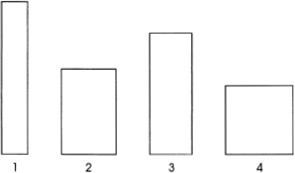
FIG. 9.1
Rectangles of various ratios of height to width.
Closely related to the Fibonacci sequence is one called the Lucas sequence. As before, each term of this sequence is the sum of the previous two terms. However, instead of starting with the numbers (1, 2) as in the Fibonacci sequence, the Lucas sequence begins with (1, 3). This yields 1, 3, 4, 7, 11, and so on.
Fibonacci Numbers and the Golden Section
In figure 9.1, four rectangles are shown with height-to-width ratios ranging from the tall slender rectangle on the left (1) to the square on the right (4). Which one of the four shapes do you like the best? That is, which, if any, do you think is the most esthetically appealing?
Well, different people like different things, but psychologists have found that most people “like” rectangle 2 best, because it is neither too slender nor too square; it “seems about right.” In any event, rectangle 2 of figure 9.1 is rotated 90° and dimension symbols added in figure 9.2.
The ancient Greeks, especially their architects, were probably the first to believe that there was a ratio between the length and the height of a rectangle that gave the most pleasing artistic proportion. Historians suspect that the famous Parthenon in Athens was designed and built with this ratio in mind.
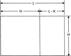
FIG. 9.2
Definition sketch for the golden rectangle or golden section.
With reference to figure 9.2, our problem commences by simply constructing the pleasing ratio
![]()
From here on, the problem is one of algebra. The above equation yields the expression L2 – HL – H2 = 0. If you remember how to solve quadratic equations like this one, you will easily obtain the answer,
![]()
So we have determined the length-height ratio of a rectangle that gives the most pleasing appearance, at least in the opinion of the early architects and artists. This ratio, L/H, has been given a special name: the golden ratio or golden section. Furthermore, since mathematicians consider it to be a very important constant, it has also been given a special symbol, ø. That is,
![]()
Now, are you ready for an interesting surprise? The numerical value of the golden section is ø = 1.618034.…Does this quantity look familiar? It is the ratio of successive Fibonacci numbers we looked at a few moments ago. Fantastic, right? Why should the breeding habits of a bunch of prolific rabbits have anything in common with ancient Greek architecture? Mathematics is not only beautiful, it can also be very intriguing!
A few more items about ø. The early Egyptians may also have been aware of the golden section. In chapter 20, “How to Make Mountains Out of Molehills,” we discuss the fact that the main dimensions of the Great Pyramids of Egypt (built during the period 2650 to 2500 B.C.) seem to conform to the geometrical proportions directly related to ø.
On quite another topic and as we established in chapter 1 the perimeter p of a regular five-pointed star of radius R is ![]() . The dimensions of playing cards are not greatly different from the ratio ø. Most books seem to have this proportion, and virtually all the flags of the world have length:height ratios close to ø:1.
. The dimensions of playing cards are not greatly different from the ratio ø. Most books seem to have this proportion, and virtually all the flags of the world have length:height ratios close to ø:1.
The golden ratio or golden number, ø, appears frequently in other quite unexpected places. Quite a few of these are discussed by Huntley (1970); here is one more. Consider a square of unit side length as shown in figure 9.3. Another square of side length x is removed from the first square. The center of gravity of the L-shaped area is at 0. What is the value of x?
This problem, proposed by Lord (1995), is solved as follows. We compute the torques (or moments) about axis 00' (or axis 00"). Equating the clockwise torques to the counterclockwise gives
![]()

FIG. 9.3
Definition sketch for a balanced area.
which yields
x2 + x – 1 = 0.
The solution to this quadratic equation is ![]() . This is the length of the rectangular leg; its width, of course, is (1 – x). A bit of algebra shows that the length-width ratio x/
. This is the length of the rectangular leg; its width, of course, is (1 – x). A bit of algebra shows that the length-width ratio x/ ![]() . Thus, the two rectangular legs of the L-shaped area are golden rectangles: an interesting result. You might want to test this answer by very carefully cutting the L-shaped area from a piece of stiff cardboard and balancing it on a needle at point O.
. Thus, the two rectangular legs of the L-shaped area are golden rectangles: an interesting result. You might want to test this answer by very carefully cutting the L-shaped area from a piece of stiff cardboard and balancing it on a needle at point O.
Finally, as illustrated in figure 9.4, suppose we start with a relatively large golden rectangle of length L and width H. We mark off the corresponding square of side length L – H. This leaves another but smaller golden rectangle. We again mark off the corresponding square. This process is repeated until we begin to approach the pole, O. Then a smooth curve is drawn through the corners of each of the squares. It turns out that this curve is what is called an equiangular spiral or logarithmic spiral. It is surely one of the most beautiful curves in all of mathematics. Let us take a closer look at it.
The Golden Section and the Logarithmic Spiral
In the branch of mathematics called analytic geometry, two basic systems are utilized to display and mathematically describe plane curves. One is the rectangular coordinate system, in which any point p is specified by its rectangular (x, y) coordinates. The other is the polar coordinate system, in which a point is identified by its polar (r, θ) coordinates. We shall use polar coordinates in our present analysis.
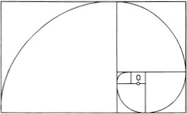
FIG. 9.4
The golden rectangle: a geometrical basis for the logarithmic spiral curve.
The pole O and a portion of the curve illustrated in figure 9.4 are shown in figure 9.5. The equation of the logarithmic spiral is
![]()
in which (r, θ) are the polar coordinates, ro is the value of r when θ = 0, and α is the angle between the radius vector r and the tangent to the curve at any point P; the symbol cot α is the cotangent a = 1/tangent α. The fact that this angle is constant all along the curve is the reason that it is sometimes called the equiangular spiral.
It is not difficult to show, using equation (9.8), that the length of the logarithmic spiral is
![]()
where sec α = secant α = 1/cosine α.
There are numerous interesting features of this beautiful curve. Perhaps the most noteworthy is that the shape of the curve does not change as it increases in size. In nature, this remarkable property is vividly displayed in the Nautilus sea shell. As seen in figure 9.6, this shell has the shape of a logarithmic spiral. Other kinds of sea shells, the horns of various types of animals, and growth patterns of sunflowers and other plants all have these spiral shapes. These and related topics are discussed by Huntley (1970) and by Thompson (1961).
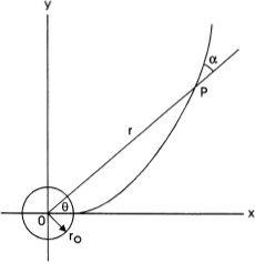
FIG. 9.5
Definition sketch for the logarithmic spiral.
We conclude our brief look at logarithmic spirals with a numerical example involving naval warfare tactics.
EXAMPLE: A DESTROYER INTERCEPTS A SUBMARINE. A destroyer sights an enemy submarine at a distance L = 4.0 nautical miles. Knowing that it has been sighted, the submarine quickly dives and heads off at maximum velocity Us = 10 knots, in a certain direction θ. The velocity of the destroyer is Ud = 30 knots. Assuming that the submarine's velocity and direction do not change, what should be the destroyer's tactics to assure an interception regardless of the direction the submarine takes?
Our example is illustrated in figure 9.7. The points D and S identify the locations of the destroyer and the submarine at the moment of initial visual contact. Now the submarine, initially at point S, immediately dives after visual contact and proceeds along some constant course, θ, at a velocity Us = 10 knots. The destroyer, initially at D, should head directly for point S at a velocity Ud = 30 knots and maintain that course for 3.0 miles, that is, 6 minutes. (Why? Hint: if the submarine were to select the course θ = 0, (that is, headed directly for the destroyer, interception would occur at point C.)
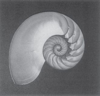
FIG. 9.6
A logarithmic spiral in nature: the Nautilus sea shell.
When the destroyer reaches point C, it should make a sudden radical course change and head initially in the direction θ = α = arccos(Us/ Ud) = 70.5°. Thereafter, the destroyer should follow the continuously changing course defined by the logarithmic spiral of equation (9.8) in which ro = 1.0 miles and cotα: = 0.3536. The spiral course of the destroyer is shown in figure 9.7.
It should be apparent that the destroyer will intercept the submarine regardless of the direction θ of the latter. You can check your calculations by using equation (9.9) to compute the distances covered by the destroyer. With this information, you can calculate interception times. A typical result: If the submarine were to select a course θ = 270°, interception would occur at a distance 5.3 miles from the original position of the submarine, 32 minutes after initial contact. The destroyer would have traveled a distance of 15.9 miles.
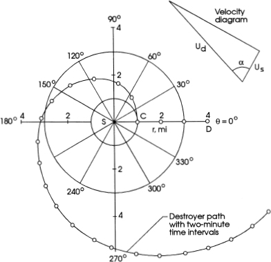
FIG. 9.7
The logarithmic spiral. Example: Naval warfare tactics.
A reminder: When computing, make certain you express θ in radians, not degrees. Recall that 1.0 radian = 360/2π= 57.3°.
Examining Hailstone Numbers
After investigating two quite ancient sequences of numbers—the prime numbers and the Fibonacci numbers—we now turn to a sequence that is relatively new: the so-called hailstone numbers.
These numbers are generated by an extremely simple mathematical process in what is called the 3N + 1 problem; it is also known as the Collatz problem and the Syracuse problem. By whatever name, it seems to have started in the 1930s, went away for a while, and then came back with renewed vigor in the early 1970s. For quite a few years it attracted the interest and efforts of many mathematicians in numerous American universities. Indeed, the joke went around in those days that the 3N + 1 problem was planted in mathematics departments by enemy agents in a diabolical attempt to divert mathematicians from serious important research. To date, the basic problem has not been solved, so people are still working on it though perhaps not as vigorously as they were before.
In any event, here is a description of the 3N + 1 problem and how it generates hailstone numbers. Select a positive integer, preferably small at the outset, for instance, less than 10 or 20. If it is an odd number, multiply it by three and add one (that's the 3N + 1 thing); if it is even, divide it by two. Keep repeating this process until you cannot go any further. Let's try a few numbers and see what happens.
a. Start with N = 3. Then, applying the rules (if odd 3N + 1; if even N/2) we generate the sequence 3, 10, 5, 16, 8, 4, 2, 1, 4, 2, 1, 4,
b. Start with N = 5. We obtain 5, 16, 8, 4, 2, 1, 4,
c. Start with N = 7. We obtain 7, 22, 11, 34, 17, 52, 26, 13, 40, 20, 10, 5, 16, 8, 4, 2, 1, 4, 2, 1,
So far, we have tried three starting numbers: 3, 5, and 7. In each case, our computations terminated when we entered a 4, 2, 1, 4, 2, 1 cycle. For the N = 7 case, we reached a maximum value of 52 and went through 16 computational steps (i.e., a path length of 16) before we reached the 421421 endless loop. Does this always happen regardless of the magnitude of the starting number? Perhaps we should begin with a larger number.
d. Start with N = 25. We obtain the sequence 25, 76, 38, 19, 58, 29, 88, 44, 22, 11, 34, 17, 52, 26, 13, 40, 20, 10, 5, 16, 8, 4, 2, 1. That's more like it! This time we reached a maximum value of 88 and a path length of 23: an improvement but not good enough.

FIG. 9.8
The hailstone numbers with starting number N = 27.
e. Start with N = 27. Well! What happened? As you will want to confirm, in this case the maximum value of the sequence was an amazing 9,232 and the path length was 111. A plot of this N = 27 sequence is shown in figure 9.8. We note that the plot displays several intermediate maximum values, notably 1,780 and 7,288, before it reaches the peak of 9.232 and then plunges to N = 1. Indeed, the entire plot of figure 9.8 looks like the great Wall Street crash of October 1929.
Incidentally, the reason these sequences are called “hailstone numbers” is because they behave something like the hail particles we associate with those enormous cumulonimbus clouds we call thunderheads. Small-diameter hail particles are caught in strong updrafts of air and are carried to great heights, growing in size as they do so. At high altitudes, these hail particles tumble out of the main current of the updraft and begin to fall, still growing in size. Near the base of the massive cloud they are again transported upward. This rising and falling pattern is repeated a few times. Finally, the hail particles become so large and heavy that they fall to the earth—something like our hailstone numbers going up and down several times before finally crashing to N = 1.
Up to here we have demonstrated that maximum values and path lengths of hailstone sequences depend somewhat on the magnitude of the starting number. More importantly, regardless of where the sequence starts, invariably it seems to get caught in the 421421 cycle and falls to N = 1.
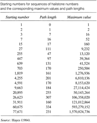
We wonder if this is always the behavior. Does the sequence always terminate with 4, 2, 1, or could it, for some starting numbers and possibly after many ups and downs, nevertheless go off to infinity? Mathematicians have not yet been able to answer this question; the general solution remains an unsolved problem. Researchers at the University of Tokyo have tested every starting number up to 1.2 trillion; the sequence produced by every one of them sooner or later enters the 421 loop and ends up at N = 1. However, the conjecture that this always happens, regardless of the magnitude of the starting number, has not yet been theoretically established. For our general information, the paths lengths and successively larger maximum values of sequences corresponding to values of starting numbers N up to 100,000 are listed in table 9.3.
The hailstone number sequence: what a pleasant and easy problem to define and to carry out mathematically! Yet, so far, the 3N + 1 conjecture has eluded rigorous proof by mathematicians. In the meantime, the problem nevertheless provides a very interesting exercise in arithmetic and point plotting for students at all levels.
Here are four references dealing with the 3N + 1 problem and hailstone numbers. The first reference is the easiest: the paper by Bruce (1978) entitled “Crazy Roller Coasters.” Then come Hayes (1984) and Lines (1990). The last reference, the most difficult, is by Lagarias (1985), with the title “The 3x + 1 Problem and Its Generalizations.” The author presents a short history of the problem and includes seventy references, most of which are not easy reading unless you're a real mathematician.
TABLE 9.3