6

Thermal Sensors

Sander (A.W.) van Herwaarden

6.1 The Functional Principle of Thermal Sensors

In this chapter we describe thermal sensors based on silicon and related technologies, having an electrical output signal. Their input signal can belong to any of the six signal domains defined by Middelhoek and Audet [1], i.e., the mechanical, magnetic, chemical, radiant, thermal and electrical signal domains. In thermal sensors, the input signal is transduced into the output signal in two steps: first, the input signal is transduced into a thermal signal, which is then transduced into the electrical output signal.

After reviewing the two types of thermal sensors in the sense of transduction types, we will describe the physics of heat transfer mechanisms, in many cases the first transduction step. Then we will discuss temperature-difference sensing elements, with the emphasis on thermopiles, since transistors are discussed in Chapter 7. Finally, the various thermal sensors are discussed with some examples and applications. A more extensive treatment of this subject can be found, for instance, in ref. [2].

6.1.1 Self-generating Thermal-power Sensors

An important distinction in thermal sensors is that between thermal-power sensors and thermal-conductance sensors. In thermal-power sensors, the input signal measured by the sensor generates thermal power in the sensor. The thermal power is also used to generate the electrical power for the sensor's output signal. Because of this, the sensor is called self-generating and cannot have an output signal if the input signal is zero. In other words, these sensors have no offset and need no biasing. Their operation takes place in three steps.

(1) The nonthermal signal C (any unit) is transduced into the thermal signal heat P (in watts), by means of a sensor-specific transduction action with transduction factor Q (in W/any-unit).

(2) The heat P is converted into the thermal signal temperature difference ΔT (in kelvins), by means of thermal resistance R (in K/W).

(3) The temperature difference ΔT is transduced into an electrical voltage U (in volts), by means of a temperature-difference sensor with a transfer factor S (in V/K).

In total, the transfer U/C (in V/any-unit) of a thermal-power sensor is described by

The psychrometer forms an exception to this three-step operation; in this sensor the nonthermal signal (relative humidity) is transduced directly into a temperature difference.

6.1.2 Modulating Thermal-conductance Sensors

In thermal-conductance sensors, the input signal C influences or modulates the thermal conductance G between the sensitive area of the sensor and the ambient. To measure the thermal conductance, the sensor is biased with a heating power P. The signal in these (so-called modulating) sensors is transferred as follows.

(1) The nonthermal signal C is transduced into the thermal signal conductance G (in W/K), by means of a sensor-specific transduction action Q (in W/K-any-unit), with G_o (in W/K) as the offset of the sensor.

(2) The conductance G is converted into a temperature difference ΔT, by means of the thermal heat P.

(3) The temperature difference ΔT is transduced into an electrical voltage U, by means of a temperature-difference sensor with a transfer factor S.

For thermal-conductance sensors, the total transfer can no longer be written in a multiplicative form; instead we find

This exposes the offset-containing character of modulating sensors. As for step (3), in some thermal-conductance sensors, the electrical signal has another form, for instance a current or resistance value, depending on the type of temperature-difference sensor used.

6.2 Heat Transfer Mechanisms

In most thermal-power sensors, the heat is generated in or on the sensor itself, and the nonthermal signal is transduced into the thermal signal in or on the sensor itself. In some sensors, the transport of the nonthermal power to the sensor involves heat transfer mechanisms. In thermal-conductance sensors, on the other hand, the conductance is influenced by the nonthermal signal in the ambient directly around the sensor, not in or on the sensor itself. Here, heat transfer mechanisms are always essential to the operation of the sensor. There are four heat transfer mechanisms [3]:

• Conduction;
• Convection;
• Radiation;
• Phase transition.

Conduction

Conduction is always present, but in thermal-conductance sensors, the first transduction step can be based on it, through the thermal conduction G_cond between the active area of the sensor and the ambient. The thermal conductance between two parallel surfaces of area A at distance D can be described by

where κ is the thermal conductivity of the medium present between the surfaces. The sensor action may be based on the effect of the physical signal on the thermal conductance via modulation of:

• The thermal conductivity κ, which depends on pressure and fluid type. Pressure dependence is used in vacuum sensors, such as the Pirani gauge. Fluid-type dependence is used in thermal conductivity and overflow sensors.
• The surface distance D. This property is used in thermal accelerometers,
• All three parameters κ, D and A, as applied in the thermal properties sensor.

Convection

Convection, the second mechanism for thermal-conductance sensors, is heat transfer to moving fluids, as in flow sensors. Usually in other sensors than these convection is not relevant. Although convection adds to the thermal conduction away from the active area, the physical principle is different from conduction, since the heat is not passed on by stationary molecules from neighbor-to-neighbor, but carried away by a continuously refreshed supply of molecules flowing past. In the simplest formula for laminar flow over a flat plate, the thermal conductance per square meter is described by

where L is a characteristic length, for instance the length of a sensor, Pr is the Prandtl number that is a temperature-dependent material constant, and Re is the Reynolds number, which depends upon the flow velocity V, the length L and the kinematic viscosity v (in m²/s), so that Re = VL/v. The sensor action can be based on the flow-velocity dependence of the Reynolds number, such as that in flow sensors. In rare cases, such as in some Pirani gauges for vacuum measurement near atmospheric pressure, the sensor action is based on the pressure dependence of the viscosity and the conductivity, which also affect the Reynolds number.

Radiation

Radiation is transfer of heat by means of electromagnetic waves, either through infrared radiation (thermal radiation), or in other forms, such as microwaves or magnetic fields which generate heat in a dissipative layer (hysteresis in a magnetic layer, for instance). It is a self-generating effect, and therefore the basis of a thermal-power sensor. Equations (6.11) and (6.12) represent two interesting formulae for infrared radiation. The first represents the heat transfer between two parallel plates, where it is around 300 K (room temperature) but with a small mutual temperature difference ΔT and assumed that one plate is a black body with emissivity ε = 1. For this case, the net heat transfer P′_ir follows from the equation:

where ε is the emissivity or absorptivity of the other plate and σ is the Stefan–Boltzmann constant (σ = 56.7 × 10⁻⁹ W/(K⁴ m²)).

The other formula describes the heat transfer between an infrared sensor with a black detecting area A_D (as viewed from the object) and an object with area A_obj (as seen from the sensor) and emissivity ε. When the detector temperature is T_D and the object temperature T_obj, the exchanged power P_ir amounts to:

Here, σ is the Stefan–Boltzmann constant and d is the distance between sensor and object. When a sensor with a sensitive area of 1 mm² at 300 K views an object at 301 K of 55 % emissivity and an object area A_obj = 0.1d², the exchanged power is 100 nW. It can be concluded that usually, at room temperature, radiation does not contribute significantly to the heat exchange of a thermal sensor with the ambient.

Phase transition

Phase transition is the last mechanism of heat transfer. An example is the heat generated by evaporation. Phase transitions are often encouraged by forced convection though, which influences the thermal conductance. Still, this is also a self-generating effect. Just like radiation, phase transitions generate their own thermal power (being negative or positive). A peculiarity of heat transfer by phase transition is that in some situations, heat can be transferred from a cold to a hot object; normally, heat flows from a hot to a cold object.

Table 6.1 gives a short overview of the heat transfer mechanisms described above, together with their typical magnitude for different mechanisms, and some remarks. It shows the large variations in magnitude among heat transfer mechanisms. In general, for room-temperature structures, much more heat is transferred by conduction and convection than by radiation. However, since the emitted infrared radiation power of objects is proportional to the fourth power of absolute temperature, at high temperatures, the situation is different.

Table 6.1 Overview of heat transfer mechanisms in microsensors and their magnitude for some typical dimensions and conditions of microsensors

In microstructures, free convection is seldom of importance, since it is a size-dependent phenomenon and insignificant in comparison with conduction in small structures. However, at very high temperatures (>300 °C), even in microstructures, free convection can lead to significant effects. Phase transitions such as evaporation should be avoided in self-generating sensors measuring other heat signals, since evaporation can give rise to significant parasitic heating or cooling even in thermal equilibrium. Readers interested in learning more about heat transfer are referred to handbooks such as ref. [3].

6.3 Thermal Structures

6.3.1 Modeling

Systematic design

In practical sensor structures, thermal effects are induced in the sensor by physical effects that interact with it. The sensitivity and accuracy of the sensors have to be as large as possible, while the influence of other physical effects, such as heat ‘leakage’ along connections and suspensions, and self-heating effects have to be minimized.

Usually it is possible to design structures in such a way that only a few well-known parameters dominate their behavior. When certain parameters are not well known, their influence ought to be negligible. Therefore, a good thermal structure design is simple and can be described by simple models. The validity of the approximations and assumptions in the model is checked by comparing the results of simulations with experimental results. When the approximations and assumptions are found to be incorrect, it does not automatically mean that a more complex model has to be used. Often it is better to change the thermal structure to avoid the undesirable influence of additional parameters!

In thermal sensors, the thermal signal is the temperature difference induced in the sensor by a physical effect. Optimizing the structure is aimed at optimizing the conversion of the power P to the temperature difference ΔT, the thermal resistance: R_th = ΔT/P. This has led to the widespread use of very thin membranes in which the thermal resistance between the physical interaction area and the ambient is maximized.

Choice and optimization of structure

When designing and optimizing a thermal structure, the choice of the thermal sensing element is an important factor, because its presence influences the thermal resistances and capacitances. For example, with transistors, diodes, or resistors in micromachined structures, connection leads can be made as thin and long as desired so that they have little influence on the thermal resistance between ambient and sensitive areas. On the other hand, a thermopile often forms both the sensing element and the thermal connection between the hot and cold areas of the sensor, and its design directly influences the thermal resistance between the ambient and the sensitive area.

An important design aspect of a sensor structure is the physical transduction process on which the sensor is based. Some sensors require large interaction areas, e.g., infrared sensors, while others hardly need any interaction area at all, e.g., true RMS converters. In thermal RMS converters, the root of the mean of the squared (RMS) value of an ac voltage or current is detected in a thermal way.

Also crucial for the structure is the packaging of the sensor chip, i.e., whether the sensor will be exposed to harsh conditions, which is often the case for flow sensors, or will be hermetically sealed, such as in case of infrared sensors and true RMS converters. Therefore, sensor vulnerability is critical during both use and production, which influences other important design criteria: the yield and the resulting cost.

Another choice involved in selecting a structure is that of technology – the choice between thin-film and silicon membranes. In general, thin-film structures are more sensitive, while silicon structures are more robust.

With respect to the interactive area, three basic structures can be distinguished:

• The closed membrane, including wafer-thick devices.
• The cantilever beam and the bridge. The latter can be considered as two cantilever beams with their ends connected.
• The floating membrane, which consists of a beam with an enlarged end.

The closed membrane has the drawback of a small effective sensitive area, but is robust. The cantilever beam and the bridge form the intermediate case, while the floating membrane has the opposite characteristics: a large effective sensitive area but a high vulnerability.

Table 6.2 Electrical equivalents of thermal parameters

Electrical-thermal analogies

The behavior of the heat flow and temperature in thermal systems is mathematically described by the same differential equations as electrical currents and voltages in electrical systems. This allows describing thermal systems by means of electrical equivalents, which is convenient because of the many excellent tools available for electrical circuit analysis and the familiarity of solving electrical-network problems.

The electrical equivalents of the thermal parameters are listed in Table 6.2, together with the SI units in which they are expressed. Note that temperature and prescribed temperature differences are equivalent to a voltage and a voltage difference, respectively, and prescribed heat flows to a current source.

Some examples of thermal resistances for different geometries are given below. Note that the thermal capacitances are simply equal to the product of the mass of the body and the specific heat. When we multiply the thermal capacitance of an element and the thermal resistance between this element and a heat source, we obtain the thermal time constant, characteristic of the time needed to heat up the element, similar to the electrical situation of capacitances and resistances. Note that there are no thermal equivalents for electrical inductance and electrical power.

Some examples of thermal resistances

Axial heat flow in bodies having an arbitrary but uniform cross-section

Let us consider the stationary one-dimensional heat flow along the axis of a body of length L and uniform cross-sectional area A (see Figure 6.1), which is exposed to a temperature difference ΔT = T₁ − T₂ between its ends.

In the steady state, the temperature distribution is given by a constant temperature gradient equal to ΔT/L, and the total heat flow through the rod is κAΔT/L. Hence, for this configuration, we find a thermal resistance R_th:

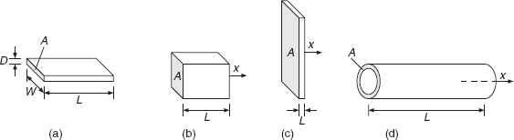
Figure 6.1 Structures with one-dimensional heat flow

This expression can be used for the one-dimensional heat flow in all kinds of structures with a uniform cross-section, such as the rods, plates or wires (Figure 6.1).

For a square plate, where the length L is equal to the width W, the thermal resistance is equal to (κD)⁻¹, which is called the thermal sheet resistance R_st of the plate.

Radial heat flow in circular bodies

Multiple thermal resistances can be combined in series or in parallel, and the resulting resistance is calculated just as in the electrical case. This method can be used to calculate complex geometries. If the geometry is such that the heat flow is one-dimensional or if a cylindrical or spherical symmetry makes it possible to assign surfaces of equal temperatures, the effective thermal resistance follows from the integration between the beginning and the end of the structure.

For instance, the thermal resistance for radial heat flow in circular bodies (see Figure 6.2) with height D can easily be found by calculating the thermal resistance of a tube-shaped cylindrical element with height D, thickness dr and radius r, which is dR = dr/(κ2πrD). The thermal resistance of a structure with inner radius r_inn and outer radius r_out can then be obtained by means of integration:

where d_out and d_inn are the corresponding diameters of the tube and 1/κD is the thermal sheet resistance of the body (tube or membrane).

Figure 6.2 Radial heat flow

Radial heat flow in spheres

The thermal resistance for a radial heat flow (see Figure 6.3) of a spherical shell element with thickness dr and radius r is dR = dr/(4πκr²). Integration between the limits r₁ and r₂ yields the thermal resistance between concentric spherical surfaces:

Figure 6.3 Spherical heat flow

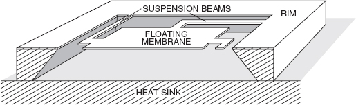
Figure 6.4 Floating-membrane structure

Numerical modeling

In many cases, a numerical solution of a model is required, since no (easy) analytical solutions are available. In these cases we model the physical situation numerically. Through electrical analogies, we can use electrical circuit analysis tools such as SPICE for time-dependent solutions. For more complex heat-flow problems, software packages such as ANSYS or other finite-element modeling packages are very useful. For relatively simple problems, one can even do numerical calculations on the PC in EXCEL, using simple software routines, based on elementary models.

6.3.2 Floating Membranes

The simplest membrane structure in terms of a thermal model is the floating membrane. In silicon, a floating membrane is made by etching a (closed) membrane in the silicon wafer. Next, a large piece of the membrane is etched free from the rim, leaving it suspended by only a few suspension beams, as shown in Figure 6.4.

The resulting large floating membrane forms the interaction area in which the nonthermal physical signal can influence the thermal signals (transduction step 1 of the sensor action, see Section 6.1.1). The suspension beams, together with any heat conduction from the interaction area to the ambient, define the thermal resistance with respect to the ambient (conversion step 2 of the sensor action). The leads of the temperature-difference transducer are incorporated in the suspension beams (transduction step 3 of the sensor action).

Thermopiles may be used in the suspension beams to measure the temperature difference between the ‘floating’ membrane and the rim at ambient temperature. The floating-membrane structure combines a very large hot area with a very high thermal resistance, because the suspension beams are usually quite long and narrow. This leads to a well-defined thermal structure having an interaction area (i.e., the floating membrane) which may be considered as an isothermal plane, connected to the ambient by some well-defined thermal resistances (i.e., the suspension beams). The large thickness of the rim to which the suspension beams are connected ensures that the beams have a perfect thermal grounding on the other side.

The thermal model

The floating membrane can be represented by a simple discrete-element model of the thermal structure (see Figure 6.5). The conductance G_beam represents the thermal conductance of the suspension beams, the capacitance C_flm represents the thermal capacitance of the floating membrane, and the parasitic conductance G_flm describes the undesired heat loss in the floating membrane caused by convection, radiation, and conduction through the gas. The variable conductance G_sen represents the desired conductance created by the physical signal.

Figure 6.5 Thermal model of the floating membrane

We can use this model to calculate the transfer function and the time constant of the floating-membrane structure. In the steady-state situation, the temperature rise in the sensor above the ambient, which results from the power dissipation P, is equal to ΔT_flm = T − T_amb = P/(G_beam + G_flm + G_sen). When the heating power is abruptly changed from zero to a constant value P₀ at time t = 0, the time response is given by:

A similar result is found for an abrupt change in (G_beam + G_flm + G_sen). The time constant τ_flm follows from the total thermal conduction and thermal capacitance:

For this simple RC time constant, the step response shows the time constant in several ways: the derivative of the curve at the step time crosses the final value after one time constant, and the curve reaches 63% of its final value after one time constant.

In general, the factor G_beam can be designed independently of the closely related parameters C_flm, G_flm and G_sen. For example, enlarging the interaction area will usually enlarge G_sen, G_flm and C_flm by approximately the same factor.

6.3.3 Cantilever Beams and Bridges

The integrated cantilever beam (Figure 6.6) is very similar in mathematical description to the uniform transmission line. Below, some simple results from this theory will be given; interested readers are referred to ref. [2].

The cantilever beam is a rectangular beam etched out of a thin membrane, attached on one side to the rim of a silicon chip and free on the other planes. This structure is characterized by a high thermal resistance between the tip of the beam and the base where it is attached to the rim. Heat dissipated at the tip of the beam will flow through the silicon to the rim, creating a temperature difference in the beam. In addition, heat may be lost to the ambient through emission of infrared radiation and conduction and convection if gases are present.

Figure 6.6 Cantilever beam structure

In vacuum, there is no heat loss from the cantilever beam through gas conduction. Supposing that also infrared radiation is negligible, then the thermal resistance R_th of the cantilever beam is given by the thermal sheet resistance R_st (= 1/(κD)) times the length-to-width ratio L/W of that part of the cantilever beam across which the temperature difference is being measured, for instance, for a thermopile of length L_tp:

Just as with the floating membrane, extending the beam beyond the thermopile can create a separate interaction region, which enhances the interaction with the physical signal to be measured. This region can be made rather large, so that the total length L of the cantilever beam can be much larger than the length of the thermopile L_tp (Figure 6.6).

Let us examine the thermal characteristics of the cantilever beam more closely. In the case of heat loss by gas conduction or infrared radiation, we obtain a thermal transmission line as mentioned above. Using transmission-line theory, we obtain the transfer function of the cantilever beam, where we define the thermal propagation constant γ as:

In this equation R_st = the thermal sheet resistance of the beam, G″_p = the shunt conductance from the beam to the ambient per unit of area, expressed in W/K m² and C″_th = the thermal capacitance of the beam per unit of area, expressed in J/K m². For low frequencies, Equation (6.20) can be approximated as:

The thermal transfer function R_th, which equals the quotient T_s/P_s of the temperature rise T_s at the tip of the cantilever and the power dissipation at the same location, is:

For small values of γL, Equation (6.22) can be approximated by the first term of a power series:

When we study the influence of parallel conduction on the thermal resistance of the beam, the term R_stG″_pL²/3 denotes the sensitivity of the transfer function of Equation (6.23) to parallel conductance. Hence, it is an important parameter for the sensitivity of the beam as applied to flow sensors and vacuum sensors. The thermal time constant τ_cant of the cantilever beam is found from Equation (6.23) by solving the corresponding homogeneous differential equation, which yields for small values of γL:

6.3.4 Closed Membranes

In closed membranes, we encounter radially directed heat transfer in a (very flat) cylindrical structure, where there is heat loss at the bottom and top of the cylinder. In the radial direction, the thermal series resistance and the thermal parallel conductance and capacitance depend on the distance from the center, where r is present in all quantities. This can be seen in Figure 6.7, where a circular membrane is assumed (practical micromachined structures are mostly rectangular). The dependence on the radius r means that there is a nonuniform transmission line for which the (relatively simple) equations of the previous section are not valid. Instead, more complicated differential equations have to be solved. We will refrain from giving the full derivation here, and refer the interested reader to standard mathematics textbooks [4]. We assume that heat is lost to the ambient by means of parallel conduction G″_p (in W/m² K) and that heat P (in W/m or in W/m²) is generated by means of dissipation in a resistor or by interaction with the ambient (infrared radiation, heat of a catalytically promoted chemical reaction). Then, if γ² = G″_P R_st, where R_st is the thermal sheet resistance of the cylindrical membrane, the general solution for the temperature is given by the sum of the modified Bessel functions:

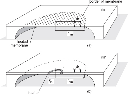
Figure 6.7 Closed-membrane structures with (a) homogeneous heating and (b) resistor heating

where A₁ and A₂ are constants dependent on the boundary conditions. K_o and I_o are modified Bessel functions of the zeroth order. There are two main cases to be discussed: homogeneous heating and resistor heating.

Homogeneous heating

Consider a closed circular membrane being homogeneously heated with a power density P″ (in W/m²), see Figure 6.7(a). As boundary conditions we use the temperature derivative in the center (which should be zero because of symmetry) and the temperature elevation T(r_rim) at the edge of the rim (by definition zero). If G″_p approaches zero, and the values of γr are small, the solution approaches:

The result is plausible since the total heat generation is proportional to P″r_rim², while the thermal resistance of the membrane is proportional to R_st.

Resistor heating

For a closed membrane in which heating with power P occurs by means of a concentric resistor (see Figure 6.7(b)) which is circular around the center and has a radius of r_in and where heat loss also occurs by parallel conduction, we obtain the following boundary conditions:

In this equation, we ignore any heat loss within the center inside the heating resistor. If necessary, a set of two equations can be defined, one of which represents the heat loss in the center inside the resistor. But even without this factor, the solution based on these boundary conditions is very complicated. We will, therefore, give the result for a design in which the heat loss due to parallel conduction (G″_p) is maximized. Extensive calculations show that this is achieved for (r_rim/r_in) = 5, which then yields:

If there is no significant heat transfer through ambient gas, Equation (6.28) simplifies to Equation (6.15) (where (ln 5)/2π = 1/4).

6.4 Temperature-Difference Sensing Elements

6.4.1 Introduction

Temperature sensing elements constitute an important part of thermal sensors. Here, we will discuss the main elements suitable for silicon and thin-film sensors that are of importance for sensor work.

For integrated sensors, mainly thermocouples and transistors are used, although diodes and integrated resistors are also sometimes used for convenience. Thermocouples and piles of them (thermopiles) have the advantage of measuring temperature differences without any offset (a self-generating measurement of the temperature difference), but they cannot measure the absolute temperature. For this, transistors are very suitable, within the operating range of −50 °C to +180 °C (see Chapter 7).

However, the fabrication of transistors requires a more complex technology than available for many microsensors and MEMS (Micro-Electro-Mechanical Structures). Therefore, also resistors made of polysilicon or thin-film metal are often used.

Integrated and thin-film resistors

As mentioned above, in most cases, thermopiles or transistors (or diodes) are the optimum choice for measuring temperature and temperature differences. Stress dependence, voltage dependence and wide tolerances make resistors less attractive. However, for reasons of temperature range or technology, resistors can sometimes be used to advantage. In silicon technology, the absolute resistance values of integrated resistors are usually not very accurate. Thin-film sensors have the advantage of a wider operating range over integrated silicon sensors, due to the absence of p–n junctions which give poor electrical isolation at high temperatures. Polysilicon and thin-film layers such as chrome-nickel or platinum are often used for the temperature-sensitive elements in thin-film sensors.

6.4.2 Thermocouples

Thermocouples are two-lead elements that measure the temperature difference between the ends of the wires. The operating principle is based on the thermoelectric Seebeck effect, which says that a temperature difference ΔT in a (semi)conductor also creates an electrical voltage ΔV:

where α_s is the Seebeck coefficient expressed in V/K. The Seebeck coefficient α_s is a material constant. By taking two wires of materials with different α_s, we get different electrical voltages across the wires, even when the wires experience the same temperature gradients. With a junction of the wires at the hot point, the voltages are subtracted, and an effective Seebeck coefficient will remain. Thermocouples or thermopiles (several thermocouples in series) in thermal sensors are made of thin-film metals or polysilicon, or monocrystalline silicon, see Figure 6.8.

Figure 6.8 Thermopile of several thermocouples of monocrystalline silicon versus aluminum

Seebeck coefficients

In practice, the Seebeck coefficient α_mono for monocrystalline silicon is related to the electrical resistivity ρ. At room temperature, this relation can be expressed as:

with ρ_o ≈ 5 × 10⁻⁶ Ω m and m ≈ 2½ as constants [5] and k the Boltzmann constant, k/q ≈ 86.3 μV/K. For practical doping concentrations, the Seebeck coefficients are of the order of 0.3 mV/K to 0.6 mV/K, where the sheet resistance depends on the layer depth.

For polycrystalline silicon, a similar expression is given by Von Arx [6] as a function of electrical resistivity:

with ρ_o ≈ 1.4 × 10⁻⁶ Ω m and m_poly ≈ 0.7 as constants, and k the Boltzmann constant. In practice, the Seebeck coefficients are of the order of 0.1 mV/K to 0.2 mV/K, for instance at sheet resistances of 50 Ω/ to 100 Ω/ and a poly thickness of 300 nm.

The absolute Seebeck coefficients of a few selected metals and some typical values of silicon are shown in Table 6.3 for two different temperatures [5, 7, 8] This table shows that the Seebeck coefficients for metals are much smaller than those for silicon and that the influence of aluminum interconnections on chips is negligible compared to the Seebeck coefficient for silicon. The electrical resistance and also the thermal conductivity play a part in determining how efficiently a thermopile functions in a thermal sensor. These parameters are much more favorable for bismuth telluride compounds or silicon–germanium compounds than for mono- or polysilicon [8]. However, the advantage of these compounds largely lies in their low thermal conductivity, compared with that of silicon, and in many microsensors the thermal resistance of the sensors is determined more by conduction through air or membranes than through the thermopile. In these, a silicon thermopile will lead to almost the same performance as thermopiles made of other compounds but has the big advantage that it can be produced in standard IC technology.

Table 6.3 Seebeck coefficients (μV/K) of some selected materials and standard thermocouples

Designing the thermopile

In a thermal sensor, the geometry of the thermopile is usually designed after the available area has been established with, for instance, length L_x and a width W. The only degree of freedom left for the thermopile design is the number of strips, or, in other words, the thermopile electrical resistance R_tp. If we neglect the area required for electrical isolation between individual strips, then for a rectangular thermopile having N thermostrips we find

Figure 6.9 Designing the thermopile

where R_se is the (technology-dependent) electrical sheet resistance. The thermopile sensitivity is Nα_s, which is the product of the number N of strips and the Seebeck coefficient α_s. Note that the sensitivity of a thermopile increases in proportion to the square root of the resistance. In other words, the resistance will increase in proportion to the square of the number of thermostrips. This is because doubling the number of thermostrips will also double their resistance, since they are halved in width, see Figure 6.9. Since the noise also increases in proportion to the square root of the resistance, the number of strips will not greatly influence the signal-to-noise ratio, and the resistance, sensitivity and number of strips can be optimized with respect to other systems parameters.

There is an optimum value for the thermostrip width, with the rule of the thumb that for efficiency's sake, the thermopile strips should certainly not be narrower than the required separation between them, and preferably much larger. In practice, thermopile resistances are chosen in the (5 to 200) kΩ range: not too high to minimize interference and the influence of the input bias currents of the electronics, and not too low to minimize the influence of the offset voltages of the electronics.

6.4.3 Other Elements

Apart from resistors and thermopiles, other elements can be used to measure temperature differences. Since there are many temperature-dependent parameters and effects, almost anything can be used. Very well-known in integrated devices are of course sensors based on transistors. With transistors it is possible to perform absolute temperature measurements (see Chapter 7). Optical effects, utilizing fiber optics or integrated optics, can be utilized, if desired in combination with a mechanical effect, such as bimetal effects or expansion, measured in an optical way. Pyroelectric materials are used in infrared sensors for burglar alarms (these sensors will only see sudden changes in the infrared irradiation). But also SAW (surface acoustic wave) resonators, and other elements are used. Generally, a direct transduction from thermal into the electrical domain is the easiest, but the technology or measurement circumstances can favor a different solution.

6.5 Sensors Based on Thermal Measurements

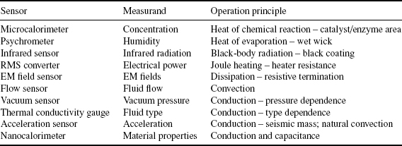
Below we will discuss the physical transduction principles of the various thermal sensors in more detail. Table 6.4 gives an overview of the different types of thermal sensors discussed below. In Table 6.4, the first five sensors are self-generating thermal-power sensors and the last five, modulating thermal-conductance sensors, which use an electrical resistance to generate heat. Except for the EM field sensor and the psychrometer, all these sensors can be realized in both silicon and thin-film technology.

Table 6.4 Overview of thermal sensors, their measurands and operation principles

6.5.1 Microcalorimeter

The microcalorimeter measures the heat that is developed during chemical reactions. Bataillard [9] describes various applications. It is possible to create a chemical reaction between two solutions in the reaction volume of the sensor (near the active area of the thermal sensor) by supplying them to this volume via two tubes. Alternatively, a catalyst or enzyme can be immobilized on the active area of the microcalorimeter, which will initiate the chemical reaction once the (single) solution comes into contact with it, see Figure 6.10. This setup ensures optimization of the transfer of reaction heat to the sensor. Even the heat produced by microorganisms, such as bacteria, immobilized near the active area of the microcalorimeter can be measured, which (of the order of 1 pW per bacterium) can be a measure of the concentration of nutrients in the solution, such as glucose, or when sufficient glucose is present, of the growth rate of bacteria.

Figure 6.10 Microcalorimeter in flow injection analysis set up (Xensor Integration)

In practice, for the glucose microcalorimeter, a transduction to the thermal domain takes place in the following two steps [10, 11]

Firstly, the concentration C (in mol/m³) of glucose in the water is converted into a reaction rate M (in mol/s) by bringing the mixture into contact with the enzyme:

where the chemical conversion efficiency dK/dt (in m³/s) depends upon the chemically active layer (catalyst or enzyme) and the particular experimental set-up. For instance, one molecule of glucose oxidase enzyme can convert at most 1000 glucose molecules per second, but it will convert fewer if the solution is not properly refreshed. When the solution is properly refreshed, the chemical conversion efficiency will depend solely on the chemically active layer (a material property) and not on the particular experimental set-up.

Secondly, the reaction rate M of the concentrate is transduced into heat of reaction P (in W) by the change in enthalpy.

The enthalpy change −ΔH is the energy freed by the chemical reaction (in J/mol) and is physically determined. For enzymatic oxidation of glucose, a value of 80 kJ/mol is found. Substitution of this value in Equation (6.34) shows that a monolayer of glucose oxidase can produce a maximum power of approximately 3 (W/m²)/(mol/m³).

6.5.2 Psychrometer

In this sensor, the relative humidity of air is detected by measuring the psychrometric temperature depression ΔT_psych of a wetted thermometer as a result of evaporation. This sensor is therefore based on a physical phase transition. The first transduction step can be described by:

Here p_dry and p_wet are the partial vapor pressures of water at the air temperature and at the wet-thermometer temperature, and P_atm is the atmospheric pressure. The size of the sensor-specific transduction factor Q is of the order of 1700 K [2, p. 184]. Equation (6.35) cannot simply be converted into the relative humidity, because ΔT_psych depends on temperature and humidity, and is much smaller than the depression of the dew point temperature. An estimate is obtained by multiplying Q by 30% × p_dry/P_atm. At room temperature with P_atm = 100 kPa and p_dry ≈ 2 kPa, the sensitivity is typically in the order of 0.1 K/%RH. To know the relative humidity precisely, a psychrometric chart is required. This can be found on the web in many forms, electronically, corrected for height above sea level.

Note that this sensor has the extraordinary feature that it transduces the nonthermal signal directly into a temperature difference. There is no conversion in the thermal domain as in all the other thermal sensors. Of course, an accurate transfer will only occur if good thermal isolation is maintained; therefore design of a proper thermal resistance is necessary anyway. Some other measures, such as forced convection across the wetted thermometer of the proper magnitude are also essential for accurate transduction. No silicon version of this sensor is known to the author.

6.5.3 Infrared Sensor

From the transduction point of view, the infrared sensor is fairly simple. The transduction from radiation to heat is carried out by a black absorber, which can have an efficiency up to 99 %. The first transduction step from incident radiation density P″_inc (in W/m²) to thermal power P is

where A_D is the sensitive area of the sensor (usually the area that is coated black), α is the absorptivity of the black coating of the sensitive area, and τ_filter is the transmittance of an infrared filter, which can be applied to select specific radiation wavelengths or simply for mechanical protection. The absorptivity α is between 0 and 1 and denotes the fraction of infrared radiation power which is absorbed by the black coating. Various types of black coatings are used for silicon infrared sensors. A simple and efficient method is to use the silicon oxide and silicon nitride layers present in all semiconductor production processes [12, 13]. Lenggenhager [12] found an absorption in the order of 50 % for radiation wavelengths of (7 to 14) μm. The use of the absorption of PVDF and its metal electrodes enables another way to implement this method [14]. Porous metal coatings are used to fabricate very black layers [15]. Gold black will absorb more than 99 % of radiation over the entire infrared spectrum. A different method is used at Xensor Integration [16]. The sensor is spin coated with a black polymer. Using techniques very similar to normal lithographic and RIE etching processes, a pattern of a 5 μm thick coating is obtained on the wafer, which absorbs about 90 % of the infrared radiation. This layer is patterned just like any other thin film on silicon and will withstand further processing of the wafer. This is in contrast to coatings such as gold black, which are very vulnerable and cannot be handled once they have been applied.

The filter with transmittance factor τ_filter is usually incorporated in the encapsulation of the sensitive element of the sensor. This filter can be broadband, transmitting infrared radiation with wavelengths between 2 and 14 μm. It can be high-pass (7 to 14) μm, for detection of objects at room temperature, which emit radiation at wavelengths of typically 10 μm (intrusion alarm). In other applications, a filter with a band-pass character is desired, transmitting, for instance, radiation at a wavelength that is in the absorption band of a gas. In this way, a gas sensor can be constructed in which the radiation intensity is measured in a reference path and in a path where the gas mixture under investigation is present. The difference in intensity is due to the presence of radiation-absorbing gas. This method is used especially for CO₂ and CO.

Infrared sensors have many applications. Burglary alarms use infrared sensors of the pyroelectric type, which respond to changes in the infrared image. This is particularly useful in security applications, where an image without any movements is the proper one and a sudden movement indicates an intruder. For gas analysis, such as CO and CO₂, infrared sensors based on thermopiles and thin membranes are used. Other applications include temperature measurement, where, for instance, the toasting of bread can be monitored using an infrared sensor. For space applications, EADS Sodern developed a focal plane array (FPA) of infrared detectors for a so-called Earth sensor, where the image of the Earth is projected onto the FPA chip using a germanium lens. The Earth sensor uses the image in the (14 to 16) μm band, emitted by the CO₂ of the atmosphere. This image of Earth is nicely round and is dependent neither on day or night nor on the seasons. In this way, the attitude of the satellite with respect to the Earth can be measured, and if necessary, corrected; as a result, for instance, a weather satellite will monitor the weather in the required region, instead of that of the North Pole or space. The FPA chip contains 132 infrared pixels (each with its own thermopile and black area) and measures 20.5 mm × 20.5 mm (Figure 6.11) [17].

Figure 6.11 Focal plane array of 4 × 32 infrared detectors for satellite attitude control instrument, chip size 20.5mm × 20.5mm (Xensor Integration)

6.5.4 RMS Converter

Thermal RMS converters are used in digital multimeters and by metrological institutes to measure the power in alternating current (ac) signals. The first transduction step, that from electrical to thermal, is simply performed by dissipation in an electrical resistor. Complications arise from the parasitic thermoelectric Thomson and Peltier effects at dc signals, and from skin effects and parasitic capacitances and inductances at high frequencies, which cause differences in the heat actually generated in the heater. By comparing ac signals with dc signals and reversing the current direction, the ac signal levels can be determined very accurately. Up to a very high grade of precision, the details of these devices have been studied by calibration engineers [18]. These authors fabricated closed-membrane structures with thin-film thermopiles and heaters for application in high-accuracy RMS converters, see Figure 6.12.

Figure 6.12 Thin-film RMS converter, w = width and t = thickness of films (courtesy of Klonz and Weimann)

6.5.5 EM Field Sensor

The EM field sensor is also a subject of study of calibration engineers. Actually, the frequency range of these sensors is in between that of an infrared sensor and an RMS converter. The infrared sensor detects (optical) EM waves at very high frequencies of around 10¹⁵ Hz; the RMS converter works for electrical signals with frequencies up to 10⁹ Hz. The EM field sensors are especially designed for the intermediate frequencies. To the best of the author's knowledge, at present no semiconductor EM field sensor is available. However, some research activities have been reported on termination of waveguides. In this research work, properly designed metal patterns on glass plates are used, which are able to convert EM field energy into heat, to be subsequently detected by a bolometer. Here, the first transduction step, that from radiant to thermal, is carried out by a specifically designed metal pattern, yielding a lossless and reflectionless termination of the wave-guide with the actual design depending upon the frequency and the wave-guide geometry [19].

6.5.6 Flow Sensor

Flow sensors are based on the transfer of heat to moving fluids. This effectively increases the overall thermal conductance between sensor and ambient. For flow sensors, the physics of the second and third step in the transduction process are just as simple as for all thermal sensors, but the similarity ends there. Both the physics of the first transduction step, from flow to thermal, and the encapsulation of the sensor are much more complicated than for most other sensors. What is more, the encapsulation greatly influences the first transduction step, because it influences the type of flow. There is laminar flow when the fluid flows along straight flow lines, and turbulent flow when it flows in irregular patterns, and the local flow direction has no direct link with the average flow direction. In microstructures, laminar flow is often encountered, although for thermal wind meters, microturbulent flow is also encountered [2; Section 6.4]. The dependence of heat transfer on flow velocity is different for laminar and turbulent flow. For laminar flow, the first transduction step can be approximated by

where G is the total thermal conductance from the sensor to the ambient, G_o is the offset (the conduction part), and H is the heat transfer normalized to the flow velocity V. As can be seen, the convective part of the thermal conductance is proportional to the square root of the flow velocity. The variable H includes parameters such as the sensor size, flow history, and fluid characteristics (viscosity, thermal conductivity, temperature).

The history of the fluid flow upstream of the sensor can greatly influence the exact flow pattern over the sensor and the sensor's heat transfer characteristics. That is why the encapsulation of these sensors has such a large influence. Even the temperature profile of the flow sensor itself will influence the heat transfer to the flow. Those interested in further details should consult ref. [2] on thermal sensors, ref. [3] on heat transfer theory and convective heat transfer in particular, and ref. [20] for an extensive overview paper on flow sensors.

An interesting application of flow sensors is the wind meter of Mierij Meteo, which is a thermal wind meter without any moving parts that measures flow velocity with an inaccuracy of a few percent and flow direction with an inaccuracy of a few degrees. Figure 6.13 shows a photograph of the meter with a typical diameter of 10 cm.

6.5.7 Vacuum Sensor

This sensor measures gas pressures below atmospheric pressure by measuring their pressure-dependent thermal conductivity. At very low pressures, when the mean distance between collisions of molecules is much larger than the distance between two surfaces, heat is transferred between the surfaces by individual molecules; and the rate of heat transfer is therefore proportional to the rate with which molecules hit the surface, which is the absolute pressure. At higher pressures (atmospheric for surfaces 500 μm apart), molecules transfer their heat not from surface to surface, but by collisions among themselves. Doubling the pressure will double the number of molecules transferring heat, but the distance over which they transport the heat (the mean free path between collisions) is halved, and the thermal conductivity of the gas is now independent of pressure. For low pressures P (in Pa), the sensor-specific transduction action can be characterized by the thermal conductance per unit of area G″.

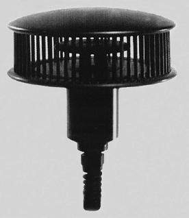
Figure 6.13 Thermal wind meter without any moving parts (www.mierijmeteo.demon.nl) (courtesy of Mierij Meteo)

Here, G″₀ is the thermal conductance per unit of area, for the reference pressure P₀ = 1 Pa, which value is typically in the order of 1 W/m²K for gasses such as nitrogen, helium, etc. For the entire pressure range, the relation between thermal conductance and pressure is:

where κ/D is the thermal conductance between two plates at distance D for a gas with thermal conductivity κ [21].

Figure 6.14 shows the thermal conductance in a floating membrane vacuum sensor as a function of pressure for three different gases. Note that the difference in thermal conductivity of the gases at atmospheric pressure is much greater than at reduced pressures, where so-called molecular thermal conductance occurs.

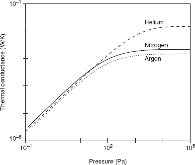
Figure 6.14 Thermal conductance of the ambient gas as a function of pressure for different gases

6.5.8 Thermal Conductivity Gauge

The thermal conductivity gauge sensor is similar to the vacuum sensor, since it measures the thermal conductance of the gas enveloping the sensor. However, in this case, the conductance does not depend upon the pressure, but at atmospheric pressure, upon the gas type (or liquid type), since all gases have different thermal conductivities. For instance, for air, the thermal conductivity is κ = 26 mW/K m at room temperature; hydrogen has the highest conductivity at more than 180 mW/K m; for helium, it is about 150 mW/K m; while gases such as argon (18 mW/K m) and xenon (6 mW/K m) are even less conductive than air. The conductivity sensor can be used in various ways. By measuring the thermal conductance it can detect the type of gas, see Figure 6.14, or it can measure the composition of a binary gas mixture. For the latter case, there is a complex formula describing the thermal conductivity of a gas mixture with volume fraction a of the first component and (1 − a) of the second [22]:

In this formula, the auxiliary variable φ₁₂ depends upon the viscosity and molecular weight of the gas molecules,

where M₁ is the molecular weight of the first gas component, and μ₁ is the dynamic viscosity of the first gas component. For φ₂₁, the indices are of course reversed.

Finally, the conductivity sensor can be utilized as a level sensor, since the thermal conductivity of a liquid is much higher than that of a gas. So the sensor can detect overflow, and might even be used to measure level in a continuous manner, although the sensor dimensions will limit the range.

6.5.9 Acceleration Sensors

Currently, there are two types of thermomechanical accelerometers to the author's knowledge. The first is very similar to capacitive accelerometers. In this mechanical thermal accelerometer, the mechanical signal (acceleration) is converted into a force F by means of a seismic mass m and a closed membrane. Subsequently the force is converted into a gap size (change) D by means of mechanical springs with spring constant K (using damping characteristics of the enveloping gas to obtain the proper frequency behavior). Finally, the gap size is transduced into a temperature difference by the thermal conductance of the gas in the gap. So, to summarize, for the accelerometer, the transfer (in steady state) will be

where A is the area of the gas conducting heat away from the sensor to the seismic mass, and G_o is the thermal conductance (offset) from the sensor to the ambient via other paths, parallel to the conductance in the gas gap. The physical principle of this thermal accelerometer does not differ much from that of the capacitive accelerometer (see Chapter 8). The gap distance is now measured thermally, instead of capacitively. This means that the first two conversion steps shown above are very similar for these two devices. The reader interested in further details on the mechanical design considerations of this sensor is referred to literature on capacitive accelerometers. Some information can also be found in [23, 24].

The second type of accelerometer concerns a design of Leung et al. [25], who have described another, very elegant, thermal accelerometer in which the seismic mass of silicon has been replaced by a seismic mass of gas, thus relying on natural convection. Usually, this is a negligible effect in MEMS devices, but this sensor is based on this physical effect. Two temperature-sensing wires are suspended in mid-air on both sides of a heater wire (all made in a MEMS process, where the wires are very narrow bridges in an etched cavity, see Figure 6.15). When there is no acceleration in the horizontal plane, the heated wire creates a hot spot of gas, which is symmetrically around the wire. When the device is not horizontal but tilted (or when the device is exposed to a horizontal acceleration), the hot gas is displaced towards one of the temperature-sensing wires, creating a thermal imbalance. This imbalance is a measure of the acceleration.

6.5.10 Nanocalorimeter

Thermal sensor structures can also be used to measure the thermal properties of thin films and of the sensor materials themselves. In general, an absolute measurement is made of the thermal resistance and the thermal time constants of a certain structure. With the modern micromachined structures, measurements have become relatively simple. These are performed in vacuum; so that only conduction in the solid material adds to the measured conductances (radiation effects are usually negligible). In this way, the thermal conductance κ and capacitance c_p of various materials has been determined, such as for silicon (150 W/K m and 700 J/kg K), silicon-dioxide (1 W/K m to 1.5 W/K m and 730 J/kg K), low-stress silicon-nitride SiN_1.1 (3 W/K m to 3.5 W/K m and 700 J/kg K), polysilicon (18 W/K m to 30 W/K m and 770 J/kg K) and aluminum (with 1 % silicon) (180 W/K m to 220 W/K m) [26–28].

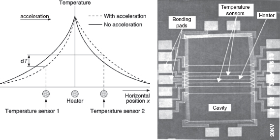
Figure 6.15 Thermal accelerometer using the ambient gas as seismic mass: (a) cross-section of the temperature distribution at the horizontal plane; (b) top view of the chip (courtesy of Leung et al. [25])

Comparable with traditional calorimeters (large laboratory bench instruments), micromachined chips such as that shown in Figure 6.16 (Xensor Integration 2005) are now used to characterize the melting and solidifying characteristics of polymers at ultra-high speeds, with heating and cooling rates up to 10 000 K/s and more [29], where the traditional calorimeters use heating and cooling rates of typically of 0.1 K/s.

Figure 6.16 Nanocalorimetric chips used for fast scanning calorimetry (Xensor Integration)

6.6 Summary and Future Trends

6.6.1 Summary

Many thermal sensors have been devised so far. Based on the heat transfer mechanisms of conduction, convection (free and forced flow) and radiation, micromachined structures have been devised using MEMS technology, often optimized with FEM modeling or modeling based on electrical analogues. By adding heaters and thermopiles, resistors or transistors as temperature-sensing elements, the thermal sensors are created. We distinguish between two types of thermal sensors: thermal-power sensors in which the physical signal to be measured brings along its own power, and thermal-conductance sensors in which the signal influences the thermal resistance between sensor and ambient. Ten different types of thermal sensors have been described.

Some of them are already much commercialized (such as infrared sensors for intrusion alarms), others are still very novel (accelerometer), or not even fabricated in silicon technology (psychrometer). Interesting also is the great difference that exists in the applicability of various thermal sensors. Infrared sensors are very simple devices because they can be hermetically sealed during encapsulation. The same applies to RMS converters, which semiconductor versions are becoming more and more popular.

6.6.2 Future Trends

For the future, breakthroughs are expected for several thermal sensors. Research on semiconductor flow sensors has by now become very impressive, but up to now the difficulties encountered by encapsulation and its influence on the sensor have obstructed a commercial breakthrough of a semiconductor version of this sensor, but make this research a scientific challenge for the future. MEMS flow sensors have already been used as detectors for gas chromatographs for many years, where the environment and flow conditions are well controlled. Application of MEMS flow sensors for the smallest flow ranges seems the most promising application of these sensors at this moment. Because of the very small chip size, these sensors are best suited for small flows. Here, a breakthrough is expected.

A revolution is taking place in the calorimeter world, where small and ultra-fast calorimeter chips can give an important additive value to widely used calorimeter instruments based on fine mechanics. The next five years will show a breakthrough for calorimeter chips in this world.

The same applies to gas measurements based on thermal conductivity measurement. Applications such as helium measurement for diving applications, helium measurement for lung function tests, and CO₂ detection are now spreading, while many other applications are expected in the near future.

Concluding, it can be said that in the field of thermal sensors, commercially, several very interesting developments are taking place, while scientifically, for sensors already developed, further refinement takes place in both performance and technology, where robustness is a main design issue.

Problems

6.1 Square thermopile design

A thermopile area measures 1.5 mm × 1.5 mm. It is made of n-type versus p-type polysilicon thermocouples, both materials having a sheet resistance of 75 Ω/. The p-type silicon has a Seebeck coefficient of +0.15 mV/K, and the n-type of −0.15 mV/K. For certain reasons it is requested that the thermopile should have an overall resistance of 7.5 kΩ. Neglect the required separation between the silicon strips.
What is the sensitivity of the thermopile?

6.2 Forced convection

Consider a flow sensor with a surface A = 1.5 mm × 1.5 mm, which at one side is exposed to laminar flow of 1 m/s. The sensor is uniformly heated, at a constant 5 K temperature increase with respect to the flow (see Figure 6.17).
Find the answer to the following question:
What is the heat transfer to the flow in this case, assuming laminar flow?
Note, that the viscosity of air v = 15 × 10⁻⁶ m²/s and that the Prandtl number of air is Pr = 0.7.

6.3 Measurement of flow direction

Consider again the flow sensor of Problem 6.2, and assume that the heat transferred to the flow upstream is 71 % and to the flow downstream is 29 %, and assume that the difference flows through the sensor chip, from halfway the downstream end to halfway the upstream end (i.e., over a distance of 0.75 mm in total). The chip is 100 μm thick silicon, and the thermal conductivity of silicon is 150 W/K m. A thermopile with sensitivity Nα_s (with N the number of strips and α_s the Seebeck coefficient), e.g., that of Problem 6.1, is used to measure the temperature difference that this heat flow causes across the chip.

(1) Calculate the output voltage of the thermopile.

(2) How is the sign of the output voltage related to the flow?

6.4 The influence of micromachining

Consider again a flow sensor chip as in Problem 6.2, but now treated with micromachining such that a floating membrane with a size of 1.5 mm × 1.5 mm and 4 μm thick silicon is inside a rim of 0.5 mm width on all sides (which may be ignored for the calculations). Again, the thermopile of Problem 6.1 is present in the floating membrane to measure the temperature difference between upstream and downstream, caused by the difference in the heat transfer coefficient. What is the first estimate for the output voltage of the thermopile now, if the differential heat flow is the same as in Problem 6.3?

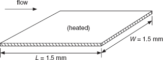
Figure 6.17 Convective heat transfer from a heated surface

6.5 Infrared radiation

Consider an infrared radiation sensor with a floating membrane sensitive area with 100 % absorptivity and an area of 1 mm × 2 mm. It views an object at 56 cm distance, with an area of 1 cm × 1 cm, also perfectly black. The sensor is at 300 K and the object is 10 K hotter. Answer the following questions:

(1) What is the net power exchange between sensor and object?

(2) What is the temperature increase of the floating membrane of the sensor, if its thermal conductance to the ambient is 330 μW/K?

(3) Make an estimate of the three major components making up the thermal conductance from the floating membrane to the ambient if the sensor is encapsulated in nitrogen, κ_N = 26 mW/K m.

(4) Estimate the improvement if the sensor were encapsulated in xenon (κ_Xe = 6 mW/K m) instead of in nitrogen?

6.6 Thermal modeling

A floating-membrane sensor has a suspension beam of 2 mm length, 200 μm in width and 5 μm in thickness (κ_Si = 150 W/K m). At its end a floating membrane is suspended with an area of 2 mm², between heat sinks at 0.5 mm distance under and above the membrane. The sensor is encapsulated in argon (κ_He = 18 mW/K m).

(1) What is the beam's thermal resistance compared with that of the floating membrane?

(2) How do the thermal time constants of the beam and the overall system (using a simple model) compare? Note that the specific heat of silicon is c_p = 1.6 MJ/m³ K.

6.7 Circular thermopiles

A thermopile is integrated in a closed silicon membrane. The membrane is monocrystalline silicon with a diameter of 3.6 mm and a thickness of 5 μm (κ_Si = 150 W/K m). The integrated silicon–aluminum thermopile has the hot junctions at a diameter of 1.8 mm, the cold junctions are at the edge of the rim at 3.6 mm diameter. The Seebeck coefficient of the silicon is 0.6 mV/K (that of the aluminum is negligible at approximately −1.7 μV/K). The sheet resistance of the silicon is 50Ω/ (again the aluminum can be ignored). What is the sensitivity of the thermopile, if its electrical resistance is 80 kΩ (if no separation between the silicon strips is required, and the aluminum does not require extra space).

6.8 Chemical microcalorimeter

A silicon closed-membrane microcalorimeter is used to measure glucose concentrations in water. For this an enzymatic layer (glucose oxidase) is deposited on the all-silicon membrane, which has a diameter of 3.6 mm and a thickness of 5 μm (κ_Si = 150 W/K m). The sensor measures the heat generated by the enzymatically promoted conversion of glucose with an integrated silicon–aluminum thermopile, for instance that of Problem 6.7. Assume a heat generation by the glucose–oxidase enzyme of 1 W/m² for a 1 mmol/l glucose solution.

(1) What is the sensitivity of this microcalorimeter for glucose?

(2) What is the resolution in a 1 Hz band?

6.9 Self-heating in a resistor

A polysilicon resistor, used to measure the temperature of a silicon chip, is located at the surface of this chip of 0.5mm thickness. It has an area of 25 μm × 25 μm. The resistor is biased with a current of 100 μA, has a resistance 3.9 kΩ and a temperature coefficient of 0.1 %/K. What is the error in the temperature measurement caused by the self-heating of the transistor? Simplify the problem by assuming radial heat flow in a half-sphere (thermal conductivity of silicon is 150 W/K m).

References

[1] Middelhoek, S. and Audet, S.A. (1989). Silicon Sensors, Academic Press, London, p. 6.

[2] Meijer, G.C.M. and Herwaarden, A.W. van (1994). Thermal Sensors, IOP, Bristol.

[3] Chapman, A.J. (1984). Heat Transfer, MacMillan, New York, 4th edn.

[4] Abramowitz, M. and Stegun, I.A. (1965). Handbook of Mathematical Functions, Dover Publications, New York.

[5] Herwaarden, A.W. van and Sarro, P.M. (1986). Thermal sensors based on the Seebeck effect, Sensors and Actuators, 10, 321–346.

[6] Arx, M. von (1998). Thermal properties of CMOS thin films, PhD thesis ETH 12743, Zurich.

[7] Blatt, F.J., Schroeder, P.A., Foiles, C.L. and Greig, D. (1976). Thermoelectric Power of Metals, Plenum, New York.

[8] Völklein, F. and Baltes, H. (1992). Thermoelectric properties of polysilicon films doped with phosphorus and boron, Sensors and Materials, 6, 325–334.

[9] Bataillard, P. (1993). Calorimetric sensing in bioanalytical chemisty: principles, applications and trends, Trends in Analytical Chemistry, 12, 387.

[10] Bataillard, P., Steffgen, E., Haemmerli, S., Manz, A. and Widmer, H.M. (1993). An integrated silicon thermopile as biosensor for the thermal monitoring of glucose, urea and penicillin, Biosensors and Bioelectronics, 8, 89.

[11] Herwaarden, A.W. van, Sarro, P.M., Gardner, J.W. and Bataillard, P. (1994). Micro-calorimeters for (bio)chemical measurements in gases and liquids, Sensors and Actuators, A43, 24.

[12] Lenggenhager, R. (1994). CMOS thermoelectric infrared sensors, PhD dissertation, ETH No. 10744, Zurich, p. 37.

[13] Müller, M., Gottfried-Gottfried, R., Kück, H. and Mokwa, W. (1994). A fully CMOS-compatible infrared sensor fabricated on SIMOX substrates, Sensors and Actuators A41–42, 538.

[14] Bauer, S., Bauer-Gogonea, S., Becker, W., Fettig, R., Ploss, B., Ruppel, W. and Münch, W. von (1993). Thin metal films as absorbers for infrared sensors, Sensors and Actuators, A37–38, 497.

[15] Lang, W., Kühl, K. and Sandmaier, H. (1992). Absorbing layers for thermal infrared detectors, Sensors and Actuators, A34, 243.

[16] Xensor Integration, www.xensor.nl

[17] Herwaarden, A.W. van, Herwaarden, F.G. van, Molenaar, S.A., Goudena, E.J.G, Laros, M., Sarro, P.M., Schot, C.A., Vlist, W. van der, Blarre, L. and Krebs, J.P. (2000). Design and fabrication of infrared detector arrays for satellite attitude control, Sensors and Actuators, A83, 101.

[18] Klonz, M. and Weimann, T. (1991). Increasing the time-constant of a thin-film multi-junction thermal converter for low frequency application, IEEE Transactions on Instrumentation and Measuremnet, IM-40, 350.

[19] Andreone, D., Brunetti, L. and Petrizelli, M. (1994). Design of a superconducting bolometer for low-power standards in the millimeter wave field, Sensors and Actuators, A41–42, 114.

[20] Oudheusden, B.W. van (1992). Silicon thermal flow sensors, Sensors and Actuators, A30, 5.

[21] Herwaarden, A.W. van and Sarro, P.M. (1988). Performance of integrated thermopile vacuum sensors, Journal of Physics E: Scientific Instruments, 21, 1162.

[22] Bird, R. B., Stewart, W.E. and Lightfoot, E.N. (1960). Transport Phenomena, John Wiley & Sons, Inc., New York, p. 258.

[23] Hiratsuka, R., Duyn, D.C. van, Otaredian T. and Vries, P. de (1991). A novel accelerometer based on a silicon thermopile. In Technical Digest Transducers ‘91, San Francisco, CA, p. 420.

[24] Dauderstädt, U.A., Vries, P.H.S. de, Hiratsuka, R. and Sarro P.M. (1994). Silicon accelerometers based on thermopiles. In Proceedings Eurosensors VIII, Toulouse, 25–28 September.

[25] Leung A.M., Jones, J., Czyzewska, E., Chen, J. and Woods, B. (1998). Micromachined accelerometer based on convection heat transfer. In Proc. IEEE MEMS Conference, Heidelberg, Germany, p. 627; see also www.memsic.com

[26] Sarro, P.M., Herwaarden, A.W. van, and Vlist, W. van der (1994a). A silicon-silicon nitride membrane fabrication process for smart thermal sensors, Sensors and Actuators A, 41–42, 666.

[27] Sarro P.M., Herwaarden, A.W. van, and Iodice, M. (1994b). Thermo-physical properties of low-stress poly- and mono-silicon and silicon nitride. In Eurosensors VIII, Toulouse.

[28] Paul, O., and Baltes, H. (1993). Thermal conductivity of CMOS materials for the optimization of microsensors, Journal of Micromechanics and Microengineering, 3, 110.

[29] Adamovsky, S.A., Minakov, A.A. and Schick, C. (2003). Scanning microcalorimetry at high cooling rate, Thermochimica Acta, 403, 55.