7

Smart Temperature Sensors and
Temperature-Sensor Systems

Gerard C.M. Meijer

7.1 Introduction¹

In smart sensors, sensing elements are combined with sensor-interface electronics on a single chip. Such a combination can be very favorable in terms of reliability, standardization of the output signal, accuracy, overall calibration, etc.. Because in some aspects the technologies for fabricating sensors and electronics are incompatible, it is not easy to make sensors smart. For instance, a problem for a smart chemical sensor is that on the one hand it should allow a good electrochemical interaction with its environment, while on the other hand the electronic circuit should be resistant against these chemicals. In a similar way, it is not easy to fabricate a smart temperature sensor for measuring very high temperatures (for instance > 300 °C), as this requires the use of special IC technologies. However, such technologies are not needed for smart temperature sensors measuring in the intermediate temperature range of –50 °C to + 180 °C. This is because, within this temperature range, the sensors can work for a long time with high accuracy and high reliability. Moreover, the sensor chip can be hermetically sealed with a metal encapsulation and yet, because of the high thermal conductivity of the encapsulation, there can be a good thermal interaction between the chip and its thermal environment. For these reasons smart temperature sensors are among the oldest types of smart sensors ever fabricated. Sometimes, for temperature sensors it is also undesirable to combine electronics and sensing elements.

This can be the case, for instance, because of extreme requirements for stability, size and packaging, or when a very wide temperature range is required. In such cases a smart sensor system could be designed consisting of a discrete sensing element, a sensor interface, and a microcontroller (Figure 7.1 and Chapter 12). Figure 7.2 shows a photograph of some typical components for smart temperature-sensor systems to be discussed in this chapter. In this book, the sensing elements of temperature-sensor systems will be considered to be integrated parts of thermoelectric structures. Therefore, related problems, such as self-heating and heat leakage along the connecting wires and the supporting material, will be considered as well.

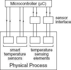
Figure 7.1 A possible system set-up with a smart temperature sensor, a discrete temperature-sensing element, a sensor interface, and a microcontroller

The main features of some commonly used discrete and on-chip sensing elements are compared in Table 7.1 and concern the following:

Discrete temperature-sensing elements

As discrete temperature-sensing elements, commonly platinum resistors, thermocouples, thermistors and transistors are used. Platinum (Pt) resistors are very stable. This is the reason why they are listed in the 1990 International Temperature Scale (ITS-90) as the interpolating temperature standard in the temperature range from 13.8 K to 962 °C. For higher temperatures, certain types of thermocouples offer better performance. Because of their low cost and high reliability, thermocouples are widely used in industrial applications for many temperature ranges. Thermocouples generate a voltage that is proportional to the temperature difference between, for instance, a reference junction and a measurement junction. This means that to measure an absolute temperature, in addition to the thermocouple output voltage one should measure the reference-junction temperature with another type of temperature sensor, which is suitable to measure an absolute temperature. However, in this case, the temperature range required of the absolute-temperature sensor can be much smaller than that of the thermocouple measurement junction. Similar arguments hold true for infrared sensors, including the popular clinical ear thermometers. As shown in the previous chapter (Equation (6.12)), the measured heat transfer depends on both the object temperature to be measured and the temperature of the IR absorber. Measurement of the temperature of an infrared-radiating object requires both a temperature-difference sensor, for instance a thermopile, and an absolute-temperature sensor, for instance a thermistor or a transistor.

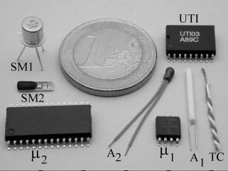
Figure 7.2 Photograph of some typical components for smart temperature-sensor systems: Pt100 resistor (A1) and thermistor (A2) with Universal Transducer Interface (UTI) and 8-bits microcontroller (μ1); smart temperature sensors (SM1, SM2) with 16-bits microcontroller (μ2); T-type thermocouple wire (TC)

Table 7.1 Important features of various types of temperature-sensing elements

Thermistors, which are not as stable as Pt resistors, are suitable for use for the temperature range of about –80 °C to 200 °C. Thermistors offer the advantage of being cheap, highly sensitive, and small in size. One of their drawbacks is their strongly nonlinear characteristic, which complicates the signal processing.

Transistor temperature sensors are as sensitive as thermistors and have the advantage that their base-emitter voltage is almost linearly related to the temperature. However, compared to thermistors, at the important temperature range around 300 K, they are less accurate and their stability during thermal cycling is lower.

Sensing elements integrated on silicon chips

As sensing elements integrated on silicon chips, resistors, thermocouples and transistors can be used. One might think about taking advantage of the favorable stability properties of platinum (Pt) and try to make silicon chips with platinum thin-film layers in order to combine Pt sensing elements with electronic circuitry. However, such a technology would be expensive and not compatible with standard IC processing. Moreover, the stability of such thin-film resistors would be inferior to that of their discrete counterparts. As an alternative, integrated diffused silicon resistors could be used. These resistors do have a temperature coefficient comparable with that of Pt resistors. However, they have the disadvantages of being stress dependent, having wide tolerances and showing a voltage-dependent nonlinear behavior. Integrated thermocouples do not measure the temperature itself, but rather difference in temperature two on-chip junctions. For absolute measurements, the temperature of one of the junctions has to be measured with another type of sensor. Nevertheless, as discussed in Chapter 6, integrated thermocouples or thermopiles are very suitable for application in many types of thermal sensors. In such sensors, a physical quantity, for instance radiation, is converted into a temperature difference, which can be measured with a thermocouple. A very useful feature of thermocouples is that intrinsically they have no offset: When there is no temperature difference, there is no voltage, so that the offset does not have to be calibrated. If absolute-temperature measurement is required, transistors are the best devices to apply as sensing elements in integrated temperature sensors. Transistors are stable and sensitive with a somewhat linear characteristic. However, for absolute precision, they have to be calibrated, or special circuit techniques have to be applied (see Section 7.7.2).

In this chapter we will firstly discuss the application-related requirements and problems of temperature sensors, including accuracy, short-term and long-term stability, noise and resolution, self-heating, heat leakage along the connecting wires, and dynamic behavior. Next we will discuss the characteristic features of temperature-sensing elements (including discrete components), smart sensors and their applications. In this chapter we will limit ourselves to temperature sensors that can perform absolute temperature measurements, being resistive sensors (Section 7.3) and transistor sensors (Section 7.4). For thermocouples, thermopiles and the corresponding thermal sensors, we refer to Chapter 6.

7.2 Application-related Requirements and Problems of Temperature Sensors

The costs of sensors are highly related to their performance. To obtain a high absolute accuracy, individual calibration of the sensors is needed, which will strongly increase their cost. Sometimes, users ask for sensors with an inaccuracy of less than 10 mK. After some discussion it turns out that they only need a short-term drift of less than 10 mK. However, the cost of the latter type of sensor will be orders of magnitude less than that of the one mentioned earlier.

In this section we will discuss the application-related problems, requirements and features of different sensors, which may help a possible user in making the right choice of sensor type, its packaging and its mounting. Properties to consider are its: (in)accuracy, short- and long-term drift, noise, self-heating, and dynamic response.

7.2.1 Accuracy

Temperature measurements with the highest accuracy can only be performed in specialized laboratories, using complex types of gas thermometers performing radiant-intensity measurements. For practical use, the international society has also developed other tools. In 1990 the International Committee of Weights and Measures adopted the International Temperature Scale ITS-90. This scale (T₉₀) allows us to compare the accuracy of practical temperature sensors with Standard Instruments, calibrated at reproducible equilibrium states, called Defining Fixed Points, and to interpolate between these fixed points [1]. One of the Defining Fixed Points is the triple point of water. This is the temperature at which the three states of water (solid, liquid and gas) are in equilibrium. This point has been defined as being 273.16 K = 0.01 °C. In between the fixed points, the practical temperature scale is defined using interpolating Standard Instruments. Between the triple point of equilibrium hydrogen (13.8033 K) and the freezing point of silver (961.78 °C) T₉₀ is defined by means of platinum resistance thermometers calibrated at specified sets of defining fixed points and using specified interpolation procedures.

Standard Pt resistors must be made of pure, strain-free, annealed platinum. Because of economical and other practical reasons, in industrial applications, much simpler Pt resistors are used. The accuracy and long-term stability of these resistors is much less than that of the standard types. For instance, according to the DIN-IEC 751 standard, the tolerances for class-A resistors are already more than ±0.15 °C (see Section 7.3). For thin-film Pt resistors the tolerances are even much larger.

Sometimes, when the conditions are favorable, it is not so difficult to achieve an inaccuracy less than 0.1 K. For example, even with a low-cost clinical thermometer for periods of more than 1 year, with thermistors the body temperature can be measured with an inaccuracy less than 0.1 K. Moreover, as will be discussed in the next subsection, in many applications the absolute accuracy is not important at all, as long as the long-term or short-term drift is small enough.

7.2.2 Short-term and Long-term Stability

In some temperature-sensor applications, having a good short-term stability is more important than a high absolute accuracy. This can be explained with the following examples.

Usually, the main part of temperature-sensor drift is caused by the cross-sensitivity to mechanical stress. When a temperature-sensitive material is in mechanical contact with another material, for instance a substrate or fixing material, having a different thermal expansion coefficient, temperature changes will cause changes in the mechanical stress. This stress will affect the characteristics of the sensing elements. This effect is not well controlled and will show a large spreading over production samples. Moreover, mechanically this effect is not stable at all. During thermal cycling, the stress can show hysteresis. Consequently, the error of the temperature sensor will also show hysteresis.

Also in smart temperature sensors (Section 7.5), mechanical stress is the main source of drift. This drift is mainly due to the unequal thermal expansion coefficients of the packaging material and the silicon chip, and mechanical instability of their connection [2]. Especially for a plastic packaging during successive heating and cooling cycles, Fruett and Meijer [2] found large hysteresis effects. With ceramic or a metal packaging, these effects could be reduced to less than 0.1 K. When the temperature range is limited to that of, for instance, clinical thermometers, the short-term and long-term drift can be less than a few milliKelvin. Moreover, it has been shown that by selecting the most favorable type of transistor and crystal orientation the mechanical cross-effects will be strongly reduced. Changes in the mechanical stress can also cause long-term drift effects when they occur over periods of many years, for example due to material alteration or chemical effects.

7.2.3 Noise and Resolution

The resolution of temperature sensors is limited by noise, which causes random fluctuations of the measured temperature. There are many physical phenomena which give rise to the occurrence of noise, e.g. thermal noise, shot noise, flicker (1/f) noise, etc. In sampled-data systems, such as most of the smart sensor systems dealt with in this book, significant noise contributors are the quantization noise of the A/D conversion process. In Section 7.6 and Chapter 10, Section 10.3.4, the behavior of these noise contributors will be discussed in more detail.

If the temperature signal has a low bandwidth, averaging over a longer measurement time can sufficiently reduce the effects of noise. Often it is sufficient to use a measurement time of less than a second to achieve a resolution of a few millikelvins. However, in many applications, users want to keep the measurement time as short as possible. As soon as a measurement is completed, the power supply can be switched off until the next measurement has to be performed. For the following practical reasons such a discontinuous measurement approach could be interesting:

(1) It saves energy in battery-operated systems.

(2) It reduces self-heating (see Section 7.2.4), because of the reduced average power consumption.

(3) In a multiplexed system, many sensors can sequentially be read out with one and the same acquisition system (see for instance the first example in Section 7.6).

(4) As soon as a measurement has been completed, the microcontroller input periphery can be used for other tasks.

When the measurement time is decreased, noise will increase, decreasing the resolution will. The following examples can give an idea of the state of the art.

7.2.4 Self-heating

A temperature sensor measures its own temperature. The sensors discussed in this chapter require electrical power for their read-out. As soon as the power supply is switched on, the sensor's temperature starts to rise due to the undesired effects of power dissipation. This electrothermal effect can be modeled according to the principles discussed in Chapter 6, Section 6.3. In the simplest case, this effect shows a first-order character, which can be modeled with the equivalent circuit of Figure 7.4(a) [3]. In this figure, the current P represents the electrical power dissipated in the temperature sensor, C_th represents the thermal capacity of the sensor, and R_th represents the thermal resistance of the sensor with respect to its environment. Figure 7.4(b) shows the temperature rise versus time, starting from the moment the power supply is switched on. This figure shows that after some time, the temperature rise approaches the asymptotic value:

Figure 7.4 (a) A first-order thermoelectric model for the effect of self-heating. (b) The temperature rise after the electrical power source is switched on

Figure 7.5 A cylindrical temperature sensor mounted in the hole of a body to measure its temperature

while the initial slope tan φ = dT/dt amounts to:

In order to decrease the self-heating effect, the thermal resistance should be as small as possible, which is achieved when the temperature sensor is in close thermal contact with the object of which the temperature has to be measured. We will illustrate this effect with the following example:

7.2.5 Heat Leakage along the Connecting Wires

Especially when there is no good thermal contact between the temperature sensor and the object the temperature of which has to be measured, care has to be taken to avoid heat leakage along the connecting wires [3]. As a result of heat leakage, the thermal environment of the wires will significantly affect the temperature of the sensor. Being aware of this, we can avoid this undesired effect by a simple means: by using a thermal compound that improves the thermal contact between the sensor and the object and by using long wires (for instance 5 cm) which are in good thermal contact with the object to be measured (by winding them around it and fixing them).

7.2.6 Dynamic Behavior

The dynamic thermal behavior of a temperature sensor depends on the underlying thermal structure of the sensor plus its thermal environment and will differ for different applications. For instance, when a clinical thermometer is used rectally, temperature measurement will just takes a few seconds and is rather accurate. When the same thermometer is applied under the armpit the measurement has been found not to be accurate at all and to take a long time. This difference is due to the smaller thermal conductance of the armpit measurement. Together with the thermal capacitance of the thermometer, this gives rise to a large time constant, which is inconvenient for the user. Together with the increased sensitivity for environmental influences, this results in poor reliability of under the armpit measurements.

Especially when a sensor is used in a gaseous environment, the thermal conductance G_sg between the sensor and the gas is rather small, which leads to a slow response. This makes it difficult to measure fast changes in a gas temperature.

The simple model of Figure 7.6 may be suitable for a first-order analysis. This simple model is only valid for the case in which little heat is transferred from the sensor to the connecting wires compared to transfer via G_sg from the sensor to the gaseous environments.

The current source P in this figure represents the electrical power dissipated by the sensor, while C_s is the sensor's heat capacitance. Suppose that the gaseous environment flows with a rate larger than a certain minimum, then the thermal conductance G_sg of a flat sensor is proportional to the square root of the flow rate [3].

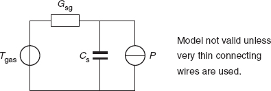
Figure 7.6 A simple model for analysing the dynamic response in a gaseous environment

In order to get a fast dynamic behavior, the sensor should be made as thin as possible: Reducing the thickness of a sensor will yield a lower thermal capacitance while the thermal conductivity is hardly affected.

To study the limitations to the response time of fast temperature sensors, Duyverman investigated the thermal properties of unpackaged chips placed in an air stream with a specified velocity (this work is described in ref. [4]). For these measurements, a 2 mm × 1 mm × 0.2 mm temperature-sensor chip was glued on a grooved printed-circuit board (Figure 7.7(a)). The observed magnitudes of the thermal conductance G_sg between the sensor chip and the gas and the thermal time constant τ = G_sgC_s have been plotted in Figure 7.7(b) versus the air velocity ν. For air velocities exceeding 1 m s⁻¹, the thermal response agrees well with that predicted by the simple model in Figure 7.6.

The experimental results show that thin naked temperature-sensor chips are suited to perform very fast temperature measurements. To keep them thin and yet to have some mechanical protection, special technology, for instance silicon wafer-to-wafer bonding, could be used to maintain this favorable property.

Figure 7.7 Testing the dynamic behavior in a gaseous environment: (a) Chip mounted on an epoxy PCB, to measure the thermal properties of uncovered chips in air streams. (b) Thermal conductance and thermal time constant of the sensor chip positioned in an air stream versus the air velocity ν

For further reading on the topics of this section the reader is referred to, for example, ref. [3]. In the next sections we will consider the characteristic properties of the most important temperature-sensing elements for smart sensors and smart sensor systems: temperature-dependent resistors and transistors.

7.3 Resistive Temperature-sensing Elements

The most commonly used elements in resistive temperature measurements are platinum (Pt) resistors and thermistors (NTCs). In this book we will limit ourselves to summarizing some practical aspects, such as the selection of the proper type, practical mathematical models and the optimum resistor value with respect to interference and self-heating.

7.3.1 Practical Mathematical Models

Platinum resistors

While the resistance of platinum is accurately related to temperature, it is also sensitive to the effects of small impurities and mechanical strain. The manufacturers of Pt resistors aim to achieve high accuracy and stability at a reasonable cost and therefore accept a certain amount of strain and impurity. Consequently, the temperature characteristics of industrial Pt resistors deviate slightly from those of pure platinum. The nominal characteristics and their tolerances are specified in various standards. For a platinum resistor R_pt, the DIN-IEC 751 standard specifies that

for –200 °C < θ < 0 °C:

and for 0 °C < θ < 850 ° C:

where

a = 3.90802 × 10⁻³(°C)⁻¹, b = 0.58020 × 10⁻⁶(°C)⁻², c = 0.42735 × 10⁻⁹(°C)⁻³

d = 4.27350 × 10⁻¹²(°C)⁻⁴, and θ is the temperature in °C. The constant R_pt(0) is the nominal resistance at θ = 0 °C. A wide range of components with different R_pt(0) values is commercially available.

According to the DIN–IEC 751 standard, the tolerances for class A resistors are given by

For a Pt100 resistor, the corresponding resistance tolerances have been plotted in Figure 7.8.

It is possible to approximate Equations (7.3) and (7.4) by the single quadratic equation [3]:

where θ₁ is a certain reference temperature which may be chosen, for example, in the middle of the temperature range of interest.

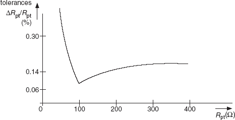
Figure 7.8 Tolerances of Pt100 resistors according to the DIN-IEC 751 class A standard

With a proper choice of the parameters θ₁, α and β for a wide temperature range, the error made by this approximation is within the tolerances of Equation (7.5). This error and the tolerances have been plotted in Figure 7.9 for three sets of parameters. This figure shows that, for a specific temperature range of interest, the parameter values can easily be optimized.

Figure 7.9 The error for Pt resistors achieved by approximating Equations (7.3) and (7.4) by the single quadratic Equation (7.6)

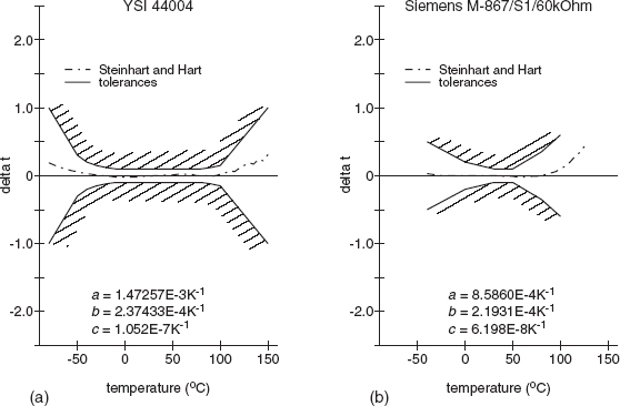
Figure 7.10 The error in °C made by approximating the nominal thermistor characteristic with the mathematical model of Equations (7.7): (a) for a YSI 44004 thermistor and (b) for a Siemens M867 thermistor

Thermistors

Thermistors, unlike platinum resistors, have not been standardized. Nevertheless, there are various mathematical models which adequately describe the resistance R_T of thermistors versus the absolute temperature T. The fitting accuracy of a number of commonly used equations has been tested and compared [3] for specified values of two types of precision thermistors, fabricated by YSI and Siemens, respectively. For both types of thermistors, the best fit has been found (Figure 7.10) with the Steinhart and Hart equation [5]:

Regarding the problems of self-heating and thermal resistance, the influence of wires and ambient-temperature fluctuations, and dynamic behavior in resistive sensors, the reader is referred to Section 7.2 and to ref. [3]. In the next subsection, we will discuss the specific problems related to nonlinearity.

7.3.2 Linearity and Linearization

In the past linear sensor characteristics used to be preferred because they simplified calculation. Nowadays, however, even the simplest of computers and controllers can rapidly calculate the temperature of nonlinear elements. The main concern with respect to linearization these days is the dynamic range of the processing circuitry, as the examples will make clear.

Another solution is to use accurate series or parallel resistors (Figure 7.11(a) and (b)). Although the accuracy of the sensor circuit is degraded by the added inaccuracy of the series or shunt resistor, the system performance may be improved because the error in the A/D converter has been reduced.

Figure 7.11 Linearization of thermistors with (a) a shunt resistor R_p and (b) a series resistor R_s. (c) The resistance R_T of a thermistor and the parallel resistance R_T//R_p versus the temperature

Figure 7.11 (c) illustrates the effect of a shunt resistance of 780 Ω for the thermistor discussed in example 7.6.

The parallel resistance R_T//R_p varies from 705 Ω to 127 Ω over the temperature range of 0 °C to 100 °C. With a 12-bit A/D converter, the resolution is 0.17 Ω which corresponds to an error of 0.05 °C at 0 °C and at 100 °C.

The value of R_s or R_p can be chosen such that the second derivative is zero in the middle T_m of the temperature range. This linearization is particularly a problem for large temperature ranges. In these cases, other types of sensors, such as Pt resistors or transistors, are preferable. For further reading on this topic, the reader is referred to, for instance, ref. [3].

7.4 Temperature-sensor Features of Transistors

7.4.1 General Considerations

There are some similarities between thermistors and transistor temperature sensors. For example, both devices are made of semiconductor material and are operated over the same temperature range of about −60 °C to +180 °C. Moreover, when the voltage is fixed, the current of both types of devices increases exponentially with temperature (Figure 7.12(a)–(c)). It appears that with this operation condition, the transistor current is even more sensitive to the temperature than that of the thermistor. Apart from these similarities, the devices differ widely. With respect to changes in the voltage V_bias, thermistors behave like resistors. In contrast to this, transistors and diodes have an exponential I_bias(V_bias) characteristic, which allows them to obtain an almost linear V_BE (T) characteristic.

With respect to applications, the most important difference is that transistor sensors can be implemented, together with electronic circuitry for biasing, multiplexing, amplification, A/D conversion, etc., on silicon smart-sensor chips.

Compared to transistor sensors, thermistors have the advantage of a higher stability during thermal cycling over, say, the 0 °C to 100 °C range. In addition, calibrated high-precision devices are available at relatively low cost.

Figure 7.12 When operated with a fixed voltage V_bias the current I_bias increases exponentially with the temperature T for (a) thermistors, (b) transistors and (c) diodes; (d) when operated at a constant current I_bias the base-emitter voltage decreases linearly with the temperature

Figure 7.13 The base–emitter voltages V_BE1 and V_BE2 of two identical transistors operated at different collector currents plotted versus the temperature T for V_BC = 0 V

In a first-order approach, there is no difference between diodes and transistors in the two-terminal configuration shown in Figure 7.12 (b). However, due to a number of physical non-idealities in the diodes, the accuracy of transistors is better. Therefore, in the following, we restrict ourselves to the transistor behavior.

Transistors lend themselves very well to be used as temperature sensors, especially when low cost, good long-term stability and high sensitivity over a limited temperature range (−55 °C to 150 °C) are required. The favorable properties of transistors for this type of application are due to the highly predictable and time-independent way in which the base-emitter voltage V_BE is related to the temperature T. The various methods for determining the temperature from V_BE can be deduced from Figure 7.13, which plots the base-emitter voltages of two identical transistors operated at different collector-current density levels against the temperature. When classified according to the method applied, there are two types of sensors, having opposite temperature coefficients:

(a) Single-transistor temperature sensors, in which the V_BE of a single transistor is a measure of the temperature.

(b) PTAT temperature sensors, in which the difference ΔV_BE between the base-emitter voltages of two transistors is a measure of the temperature (and in which the voltage is proportional to the absolute temperature (PTAT)).

Any linear temperature characteristic can be realized by amplifying and adding the voltages mentioned under (a) and (b). This property is utilized in smart temperature sensors (Section 7.5).

7.4.2 Physical and Mathematical Models

Let us assume that the collector-base voltage of the sensor transistor is biased at 0V. This is desirable because, due to the so-called Early effect, changes in the collector-base voltage affect the base width (base-width modulation) and therefore the base-emitter voltage. In this case it holds that

where A_e is the emitter area, J_s is the saturation-current density which depends on the doping profile, T is the absolute temperature, q is the electron charge, and k is Boltzmann's constant (k/q = 86.17 μV K⁻¹).

The saturation-current density J_s is strongly dependent on the temperature. This is taken into account in the well-known equation [6]:

where V_g0 is the extrapolated bandgap voltage at 0K, η is a constant which is somehow related to the doping level, and C″ is a constant. With empirical values for η and V_g0, this equation describes the I_C(V_BE,T) characteristic very accurately [7, 8]. Typical empirical values for the parameters V_g0 and η are 1160 mV and 4, respectively. The sensor transistor has to be biased at a collector current with a well-known temperature dependence. In practice it is quite easy to create a current that is constant or proportional to some power of T. Therefore, we suppose that:

For further analysis, it is convenient to express V_BE (T) as the sum of a constant term, a term proportional to T and higher-order terms, in such a way that the linear terms represent the tangent to the V_BE (T) curve for T = T_r (as shown in Figure 7.14 (a)). It can be calculated that [4]:

In this equation the following relation is valid:

To get an impression of the magnitude of the different terms of Equations (7.11) and (7.12), we substitute V_g0 = 1160 mV, η = 4, and, for example, m = 0(I_C = constant), T_r = 323 K and V_BE(T_r) = 547 mV; then we find for the constant term V_BE0 = 1271.3 mV and for the PTAT term λT in (7.11) that λ = −2.24 mV K⁻¹. The nonlinearity in V_BE (T), which is represented by the last term in Equation (7.11), is plotted in Figure 7.14(b) against the temperature in °C for various values of (η − m). This figure clearly shows the characteristic parabolic shape of the nonlinearity. This figure also shows that, with λ = −2.24 mV K⁻¹ and η – m = 3, the maximum nonlinearity over the −55 °C to 150 °C temperature range amounts to about 20 °C. This means that for such a wide temperature range, the nonlinearity should be taken into account. In smart temperature sensors this nonlinearity is usually compensated in the hardware.

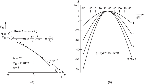
Figure 7.14 (a) The base–emitter voltage V_BE versus the temperature T. The curvature is exaggerated in order to clearly indicate the characteristic points. (b) The nonlinearity (η – m)(kT/q){(T – T_r)/T) – ln(T/T_r)} of V_BE (T) versus the temperature θ (°C)

7.4.3 PTAT Temperature Sensors

In addition to the base–emitter voltage V_BE the difference ΔV_BE between the base–emitter voltages of two transistors can also be used as a measure for temperature (see Figure 7.13). When comparing the use of these two voltages, the following advantages and drawback can be found:

• The voltage ΔV_BE is much smaller than the voltage V_BE and therefore more sensitive to noise and interference.
• The voltage ΔV_BE is immune to variations in doping concentrations and therefore its tolerances are much smaller than those of the voltage V_BE. This is important when using uncali-brated sensors (see Section 7.4.5).
• The two voltages have opposite temperature coefficients. Therefore, after amplification of the voltage ΔV_BE, the amplified voltage can be used to compensate for the temperature dependence of V_BE, which results in a temperature-independent voltage, which can be used as voltage reference (the so-called bandgap-reference voltage).

Figure 7.15(a) shows the principle of a circuit generating the voltage ΔV_BE. In such a circuit is important that all of the transistors have the same temperature T. This can easily be accomplished when the circuit is realized on a single chip, as an integrated circuit. Because the transistors Q₁ and Q₂ are operated at the same temperature T, we know from

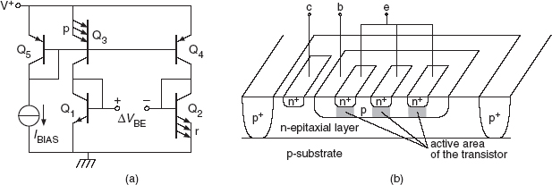
Figure 7.15 (a) Principle of a circuit to generate the difference ΔV_BE between the base-emitter voltages of two transistors Q₁ and Q₂. (b) Cross-section of a multi-emitter transistor. The active areas of this transistor are connected in parallel so that the behavior of such a transistor is similar to that of a number of parallel-connected ones

Equation (7.8) that:

For identical transistors fabricated on the same chip it holds that J_s2 = J_s1. To realise an accurate emitter area ratio r = A_e2/A_e1, transistor Q₂ has been implemented as a multi-emitter transistor, with r emitters connected in parallel (Figure 7.15(b)).

Furthermore, in this circuit, the transistors Q₄, Q₃ and Q₅ are operated in a so-called current-mirror configuration. Because of the interconnected base-emitter terminals and the equal temperature T, the collector-current densities of these three transistors are equal. Because transistor Q₃ has been implemented as a multi-emitter transistor, with p emitters, the collector-current ratio I_C3/I_C4 = I_C1/I_C2 is kept at a constant accurate value p, which does not depend on temperature or other physical parameters. Taking into account these features, Equation (7.13) can be rewritten as:

This voltage is proportional to the absolute temperature (PTAT). With this basic principle PTAT current sources can be built. Figure 7.16(a) shows a basic PTAT current source, in which the PTAT voltage is generated over resistor R₂. This circuit generates its own biasing currents: Once a certain small amount of start-up current is flowing, the currents and voltages will converge to their final stationary values.

The properties of PTAT current sources were used in the first integrated temperature sensors, in which the sensing element was integrated together with the electronic processing circuitry on the same chip [9]. These sensors provide a calibrated PTAT output current of 1 μAK⁻¹, which is stabilized against changes in the supply voltage.

Some very accurate PTAT current sources have been shown in Figure 7.16(b) [10] and Figure 7.16(c) [11]. Characteristic for these circuits are: the cross-connected bases of Q₁ and

Figure 7.16 PTAT current sources: (a) basic principle; (b) principle of an all-npn PTAT current source, (c) an all-npn PTAT current sink, (d) all-npn current sink with biasing circuit

Q₂, the unequal emitter areas with ratios r₁ and r₂ for the transistor pairs (Q₂, Q₁) and (Q₃, Q₄), and the emitter resistances R₂ and R₃. For the circuit of Figure 7.16(b), it holds that

where the numerical subscripts correspond to those of the components.

Momentarily ignoring the base currents and the base-widening effect, we find, with V_be = (kT/q)ln(I_C/I_s), that

where r₁ = I_S2/I_S1 and r₂ = I_S3/I_S4, ratios which are not temperature dependent. When R₃ = R₂ = R, we can write:

where I_o denotes the output current.

Some important conclusions may be drawn from Equation (7.17):

(a) The output current I_o is PTAT, assuming that R is temperature-independent.

(b) The output current I_o is independent of the bias current I_bias.

This remarkable feature is due to the cross-connection of the bases of Q₁ and Q₂. Another interesting circuit is obtained if R₃ = 0 Ω (Figure 7.16(c)). Equation (7.16) shows that in this case, the right-hand branch current I_E2 and therefore also I_C4 are PTAT. The circuit can generate its own biasing current using a current mirror, as shown in Figure 7.16(d). The current mirror can also be used to make available more than one PTAT current.

Figure 7.17 Generating of PTAT-voltages in CMOS technology, according to [12]

The circuits of Figure 7.16 are typical examples of bipolar designs. At the time they were designed, it was believed that low-frequency high-precision circuits could only be fabricated in bipolar technology. For economical reasons, designers tried to make similar circuits in CMOS technology. For precision application, CMOS technology has two major disadvantages:

• Because of the large mismatch of CMOS components, basic circuits such as current mirrors and operational amplifiers show a large offset,
• Because CMOS transistors are surface devices, the current through CMOS transistors shows strong flicker (1/f) noise.

Fortunately, designers found ways to reduce the effects of these basic drawbacks. Nowadays, the performance of many CMOS precision circuits is similar to or even better than that of their bipolar equivalents. As an example, Figure 7.17 [12] shows a PTAT voltage generator fabricated in CMOS technology. In most CMOS processes it is possible to apply parasitic pnp-substrate transistors to generate the PTAT voltage and V_BE voltages. By a proper setting of the switches, the CMOS current mirror M_in, M₁–M₄ takes care that the current through Q₂ is three times that through Q₁. Consequently, a PTAT voltage is generated between the emitters of Q₂ and Q₁, which nominally equals

However, due to component mismatch between the transistors, an unpredictable error will occur. Application of dynamic element matching (DEM)³ solves this problem. With this method, using switches S_p1 to S_p4, the transistors M₁–M₄ are sequentially interchanged so, that during one measurement cycle, each of them has been in the position of biasing Q₁, while the others are biasing Q₂. After a complete cycle the average value of ΔV_BE for the four permutation steps equals the desired value of Equation (7.18). In a smart sensor system, after A/D conversion of the signals, the average can be calculated in the microcontroller. This technique works so well that it is even possible to remove any cascoding transistors that would be needed for fully bipolar PTAT circuits. This will lower the minimally required supply voltage and makes the circuit suitable for low-voltage design.

Figure 7.18 (a) Principle of a circuit generating a reference voltage; (b) Principle of a circuit generating a voltage at a °C, °F or another scale. (c) The generated voltages and their tolerances versus the temperature

7.4.4 Temperature Sensors with an Intrinsic Voltage Reference

In smart temperature-sensor systems (see Section 7.5), the temperature-sensitive voltages are converted into dimensionless digital quantities. This means that somewhere in the signal processing chain a feature has to be implemented for calculating the ratio of the sensor voltage and a reference voltage. Such a reference voltage can be generated using a bandgap-reference circuit, in which a compensating voltage V_C(T) is added to V_BE(T), to compensate for at least the first-order temperature dependence of V_BE(T). This correction voltage is obtained by amplifying the PTAT difference ΔV_BE (see Equation (7.14)) of the base–emitter voltages of two transistors operated at unequal collector-current densities with ratio pr. In this way, a temperature-independent output voltage V_ref is obtained, for which it holds that

On the other hand, by inverting the V_BE(T) voltage and adjusting the scale factor A, a temperature-dependent voltage V_T(T) on a °C, °F or another scale can be obtained.⁴ Figure 7.18(a) and (b) shows two basic circuits to generate a reference voltage and a temperature-sensitive voltage, respectively. Figure 7.18 (c) shows the obtained output voltages. These voltages, V_BE(T) and ΔV_BE, show production tolerances, which will cause some inaccuracy of the voltage V_ref and V_T(T). The next subsection will discuss how calibration and trimming can reduce the effects of these tolerances.

7.4.5 Calibration and Trimming of Transistor Temperature Sensors

Because of production tolerances in the base geometry and in the doping profile, the base–emitter voltage and to a much lesser degree the PTAT voltage will show some spreading (Figure 7.18(c)). Applying DEM, according to the principle of Figure 7.17, significantly reduces the effects of tolerances in the PTAT voltage. Unfortunately, this technique cannot reduce the spreading in V_BE(T). For both voltages V_BE and ΔV_BE it holds that their extrapolated values at 0K are well known and show hardly any tolerances. Owing to this very important property, it is sufficient to calibrate and trim transistor sensors at a single temperature T_trim, to make the transistor characteristic equal the nominal one. During the calibration procedure, the base–emitter voltage and the transistor temperature are measured with accurate equipment. Then, the base–emitter voltage can be adjusted to its desired value by adjusting the biasing current or the emitter area of the bipolar transistor generating the V_BE(T) voltage. The trimming data are permanently stored in, for instance, Zener diodes that can be ‘zapped’. After zapping the Zener diode is permanently and reliable short-circuited with a small aluminum wire (see also Section 7.5.1). Alternatively, trimming can be implemented using flash EPROM, laser-trimmed thin-film resistors, or fusible links. In case of a bandgap voltage reference, it is not necessary to measure the temperature to trim the output voltage. At a temperature T_trim it is sufficient to trim the output voltage to its nominal value V_ref. When trimming V_ref of a bandgap reference or V_T of a temperature sensor, it is also possible to compensate for a possible deviation in the PTAT voltage with an adjustment of V_BE(T). This property is a consequence of the fact that the extrapolated zero-Kelvin values of both V_BE(T) and V_T(T) are not affected by the trimming procedure independently of whether V_BE(T) or AΔV_BE is trimmed.

7.5 Smart Temperature Sensors and Systems

In smart temperature sensors, temperature-sensing transistors are combined with signal-processing circuits, voltage references, trimming circuits and interface circuits to enable direct read-out by a microcontroller or a DSP (see the system set-up of Figure 7.1). A powerful feature of smart sensor systems is that they allow easy combination of the measurements of various signals, which will yield a more reliable or advanced system. For instance, in thermocouple measurement systems not only the thermocouple-output voltage is measured, but also the reference-junction temperature (Chapter 10, Section 10.6.3). In this way it is possible to perform an absolute temperature measurement. To monitor corrosion effects, the thermocouple resistance can be measured. An increasing resistance indicates that the performance is degrading. When the resistance is too large, an alarm can be triggered. From a technological point of view it is possible to fabricate smart temperature sensors with a complete on-board microcontroller. However, in view of self-heating effects, care has to be taken to limit the power dissipation. Moreover, from an economical point of view it is often preferred to use off-the-shelf microcontrollers and a universal sensor interface, which can support a number of sensing elements. Usually the sensor interface contains a period or duty-cycle modulator, or a sigma-delta converter. In addition to this, a sensor-bus interface (I²C, SPI, μWire, etc.) could be added. The sensing elements can sometimes be fabricated on the same chip, together with the interface. But often the use of discrete sensing elements is preferred (Figure 7.1). In this chapter we consider all of these options.

7.5.1 A Smart Temperature Sensor with a Duty-cycle-modulated Output Signal

Figure 7.19 shows a photograph of one of the first smart temperature sensors designed to be read out by a microcontroller. The top area of the depicted chip shows a big capacitor with a value of about 500 pF, which is used for integration of current. The row of bonding pads at the bottom side of the chip is used for trimming, using Zener diodes that can be ‘zapped’ (Zener-zapping) during the testing procedure. The sensor contains a group of temperature-sensing transistors that generate the basic voltages V_BE(T) and AΔV_BE(T) [13]. These voltages are converted into currents, which are amplified, added and subtracted as shown in Figure 7.20(a). The final result of this operation are the two currents I₁(T) and I₂(T), which have opposite temperature coefficients and are almost linearly related to the temperature (Figure 7.20(b)). The parameters C₁, C₂, R_BE and R_PTAT fulfil certain conditions, to make I_ref(T) = I₁(T) + I₂(T) independent of the temperature. The two currents I₁(T) and I₂(T) are used to charge and discharge a capacitor between two threshold voltages Figure 7.21(b). The switch is activated when the capacitor voltage crosses one of two threshold voltages. The time interval t_i between two threshold crossings amounts to

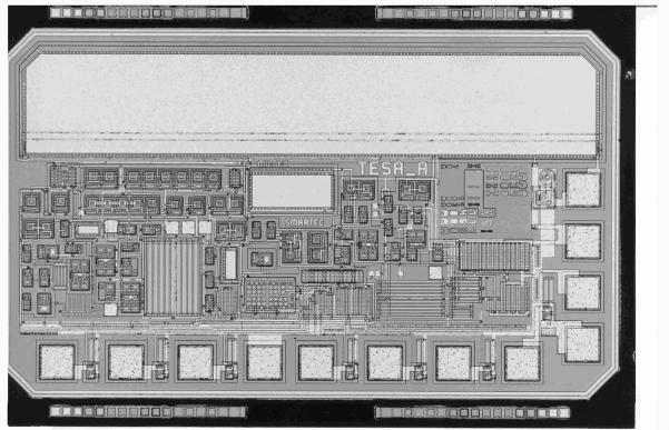
Figure 7.19 Photomicrograph of the smart temperature sensor SMT160, fabricated in BICMOS technology. (Courtesy of Smartec)

Figure 7.20 (a) Principle of signal generation of I₁ and I₂. (b) Temperature dependence of I₁ and I₂ extrapolated to 0K

where V_h is the hysteresis voltage of the Schmitt trigger which equals the peak-to-peak value of the saw-tooth-shaped voltage V_C and the difference between the threshold voltages. In this way the circuit of Figure 7.21(a) works as a relaxation oscillator. For the duty-cycle M(T) of the square-wave output signal it can be found [13], that

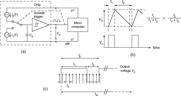
Figure 7.21 Principle of a smart temperature sensor with duty-cycle modulated output signal. (a) Basic circuit. (b) The voltage across the capacitor V_c. (c) The output voltage V_o and sampling pulses versus time

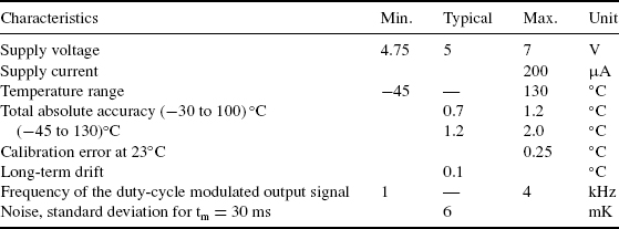
Table 7.2 Specifications of the smart temperature sensor SMT 160 (Smartec, 2006-1)

where T_H and T_L represent the maximum and the minimum temperature of the extrapolated measurement range, respectively (i.e. the range for which the duty-cycle M(T) varies from 0 to 1). In the design of the chip, some measures have been taken to compensate for the small nonlinearity of the voltage V_BE(T). The chip has been designed, such that the duty cycle varies linearly over the temperature range according to the equation:

where θ is the temperature in °C. The sensor is calibrated and trimmed during the testing procedure. The main specifications have been listed in Table 7.2.

The noise of the sensor has a flat spectral density with a standard deviation σ_sensor which depends on the number of measured periods N and amounts to:

In addition to this noise, sampling noise will also occur (Figure 7.21(c)). This noise has the same origin as the quantization noise in A/D converters and arises as follows: The microcontroller counts sampling pulses during the time intervals that the output signal is high. The number of pulses is stored in a ‘1’ register. A second register keeps track of the total number of sampling pulses during the measurement-time interval t_m. When the contents of the second register exceed a certain value, the counting is stopped as soon as t_m reaches a whole number of periods. To find the temperature θ, in the microcontroller, division (7.21) is performed and the result is substituted in Equation (7.22). Because the sampling pulses are not synchronized with the output signal, there will be some uncertainty about when the time intervals start and stop. This uncertainty is responsible for the sampling noise (see also Section 7.2.3). Straightforward calculations show that this sampling noise causes an error in the duty cycle, in which the standard deviation σ_sn

where t_s is the sampling time, t_p is the period of the signal, and t_m is the total measurement time, which equals an integer number of periods of the output signal.

7.5.2 Smart Temperature-sensor Systems with Discrete Elements

When instead of integrated temperature sensors the use of discrete sensing elements is preferred (see Sections 7.1 and 7.2), then for a number of reasons it can still be desirable to use the measurement techniques described in Chapter 2. Possible reasons for such a choice could be the wish:

• to have a microcontroller-compatible output signal;
• to minimize size, costs and power consumption;
• to implement auto-calibration;
• to have ac excitation instead of dc;
• to have a fast controllable measurement speed;
• to combine the sensor system with a control system, using the same microcontroller.

In such a case it will be of interest to consider using a special sensor interface, such as the universal sensor interface UTI, discussed in Chapter 2 [14]. These measurement principles can partly be found in the alternative interface products of refs [15–18]. For more information the reader is referred to Chapter 10 and to the websites of the manufacturers.

In Chapter 10, Section 10.6.3, it is shown how the discussed measurement techniques can be applied for a system to measure thermocouple signals. In this system the principles of transistor sensors (Section 7.4) have been applied for both the generation of the required reference voltage and the measurement of the reference-junction temperature.

7.6 Case Studies of Smart-sensor Applications

In this section we will discuss the features of smart temperature sensors for some characteristic applications. The first application concerns detection of the presence of micro-organisms, by measuring the heat they generate. The second application concerns a very precise and fast control system for stabilizing the temperature of a ceramic substrate.

7.6.1 Thermal Detection of Micro-organisms with Smart Sensors

Sterilized products must be completely free of micro-organisms. To check the quality of the production process with respect to sterility, random samples are taken from the production lots and tested. In case of packaged products, such tests must be performed in a noninvasive way in order to limit product loss, to reduce the amount of work and to eliminate the risk of infection during testing. Typically, the number of micro-organisms shows an exponential growth (Figure 7.22). During growth, the organisms use nutrients (food) and produce heat. At a certain moment t_c the growth stops, because there are too few nutrients or because the concentration of waste products is too high.

Because of their metabolism, micro-organisms can be detected noninvasively by measuring the product temperature and comparing this temperature with that of sterile reference products. Just for this purpose, a calorimeter has been designed [19] to detect the presence of micro-organisms in cartons of sterilized milk using the smart temperature sensors dealt with in Section 7.5.1.

For this particular application, typical requirements for the temperature sensors are that temperature changes as low as a few millikelvins have to be detected. Also, the effects of noise and self-heating of the sensors should be less than 1 mK. On the other hand, the absolute accuracy does not need to be very high, as long as the short-term drift over four days is less than about 2 mK. Finally, the system has to contain many sensing elements that can be easily be multiplexed and connected to a microcontroller. To illustrate typical problems in temperature measurement systems, the various design aspects will be discussed below.

Figure 7.22 The exponential growth of micro-organisms in a certain amount of liquid

Thermal considerations

The products in the calorimeter are thermally insulated from each other and from the environment. The thermal insulation has the following functions:

• The heat production of the micro-organisms causes the temperature to rise. The temperature rise increases with the thermal resistance between the milk product and the environment. Therefore, good thermal insulation results in a large thermal signal, which makes accurate detection possible.
• Thermally insulating the products well with respect to the environment ensures that the detected changes will be caused by heat dissipation in the products and not by temperature changes in the environment.
• When there is good thermal insulation between the products, it is easier to distinguish the thermal behavior of each product.

In the experiments polystyrene foam was used as the insulation material. Enlarging the contact area with the sensor can reduce the influence of the thermal resistance of the milk carton. This can be accomplished by using a metal plate. To ensure good thermal contact, we applied a special version of the smart sensors, bonded on a flat, thermally conducting ceramic substrate [20] (Figure 7.23(b)). In the first experiment, a simple experimental calorimeter for two one-liter cartons of milk (Figure 7.23(a)) was devised to measure the heat production of the micro-organisms and to test the accuracy of the thermal model (Figure 7.23(c)). This equivalent model was composed according to the principles presented in Chapter 6.3. For the details of this model the reader is referred to [19]. Each carton of milk is represented by a Π-network of two capacitors and a resistor R_c.

The resistor R_v represents the thermal resistance of the insulating wall between the cartons and R₁ and R₂ that of the insulating walls between the cartons and the ambient. The voltage source V_amb represents the changes in the ambient temperature. The current source I_m represents the power dissipation P of the micro-organisms in carton 1, which has been determined experimentally for a number of micro-organisms.

Smart temperature sensors

According to the principles described above, a calorimeter for 100 one-liter cartons of milk has been fabricated. The temperature of each carton is measured with a smart temperature sensor of the SMT 160 type [20]. Compared with resistive sensor elements, such as thermistors and Pt resistors, these sensors offer a number of advantages: The output signal is immune to resistances of electronic switches (multiplexers) and connecting wires switches, and insensitive to the effect of electromagnetic interference.

Furthermore, fewer wires and electronic switches are required. Another important advantage is that these sensors can directly be connected to microcontrollers. A block diagram of the electronic circuitry is shown in Figure 7.24. One of the smart sensors is selected with the power-supply multiplexer, via a pair of switches connected in a 10 × 10 array. All of the sensor outputs are connected to an OR gate. The signal of the selected sensor is transferred to the gate output and the microcontroller TIMER input.

As temperature changes as small as a few milliKelvin should be monitored, special attention has been paid to those sensor nonidealities that affect the resolution, such as noise and self-heating. Other sensor nonidealities, including drift and transient behavior, do not pose significant problems [19].

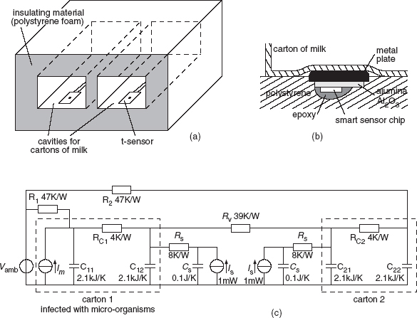
Figure 7.23 A calorimeter for the detection of micro-organisms in milk. (a) Experimental structure. (b) A sensor set-up that ensures a good thermal contact with the product. (c) An electrical model of the thermal characteristic

Noise

With the help of a short computer program the microcontroller can sense whether the sensor voltage is high or low. The speed of this sampling process is limited due to the limited timer rate and the finite instruction time of the microcontroller. This creates sampling noise, as explained in Section 7.5.1. To achieve the required accuracy it is necessary to sample over more than one sensor period. If a microcontroller of the 87C51FA type is applied and a measurement time of for instance 30 ms, the data will correspond to those used in Section 7.5.1, Example 7.7, where the sampling noise was found to be σ_sn = 8.6 mK and the total measurement noise σ_total ≈ 10 mK.

Figure 7.24 Block diagram of the sensor system

Lengthening of the measurement time t_m, which increases the number of periods N, will reduce both types of noise inversely proportional to the square root of time t_m. Because slow temperature changes are to be detected, it should not be a problem to use a longer measurement time and to reduce the noise up to any acceptable level. However, applying continuous power over a long measurement time would cause an unacceptably large error due to self-heating, as explained below. Therefore, the sensors in our calorimeter are sequentially powered for the optimal time of 30 ms each and the results are averaged over 100 measurements. This averaging reduces the noise by a factor of 10, so that the resulting total noise amounts to σ_total,100 = 1 mK.

Self-heating

When the sensor is powered, the sensor temperature starts to rise because of the self-heating caused by the internal dissipation of 1 mW. The magnitude and speed of this temperature rise depend on the thermal resistances and capacitances of the sensor and its environment. For the thermal set-up of Figure 7.23(c) with continuous powering, self-heating causes a temperature rise of up to 80 mK (Figure 7.25). The magnitude of this effect spreads, because it depends on the sensor's thermal contact to the product under test. Therefore, this effect should be reduced. The problem of self-heating is avoided by sequentially powering each sensor for period of only 30 ms [19]. A detailed analysis of the thermal structure shows that during the first 30 ms, a mean temperature rise of about 4 mK is to be expected. This error is mainly determined by the intrinsic thermal properties of the sensor itself, such as the thermal capacity of the chip and the thermal resistance from the chip to the ceramic substrate. From sensor to sensor, these short-term heating effects will only show slight differences. Therefore, as will be discussed later, when calculating the temperature differences between the various products, this effect is reduced to an insignificant level.

Figure 7.25 The self-heating effect of a smart temperature sensor in the thermal set-up of Figure 7.23(b) versus the time after the power has been switched on

Figure 7.26 (a) The measured temperatures of a row of ten cartons of milk. (b) The temperature differences between neighboring cartons calculated for the data plotted in (a), with nulling at the start of the experiment

Measurement results

Tests were conducted on the prototype with 100 cartons of milk. Figure 7.26(a) shows the temperature changes over a period of 50 hours. Because of temperature changes in the laboratory, all of the measured temperatures show a variation of a few degrees. However, the behavior of one of the cartons differs from that of the others. This carton has been injected with micro-organisms of the type Streptococcus Cremoris. By smart data processing, this effect can be distinguished more easily. This is shown in Figure 7.26(b), using the data of Figure 7.26(a). However, in Figure 7.26(b), the differences have been plotted between the temperatures of neighboring cartons of milk, with nulling at the start of the experiment. With this type of data processing, even when uncalibrated sensors are used, temperature changes as low as 5 mK can be monitored, which enables sensitive monitoring of the activities of many types of micro-organisms.

7.6.2 Control of Substrate Temperature

Surface acoustic wave (SAW) delay-line oscillators are very suited to measure interrelations between concentrations of specific gaseous chemical compounds in a carrier gas [21]. Adsorption and resorption processes of doping gasses in a chemically sensitive film, deposited on a SAW delay line, influence the phase velocity through mass and conductivity changes of this layer. Unfortunately, SAW devices are burdened with temperature cross-sensitivity, because temperature variations also change the phase velocity. A better performance is obtained by the addition of a reference delay line. However, the two delay lines will never match exactly. Therefore, there is a difference in phase velocity between the two delay lines, which is also temperature dependent. This phenomenon reduces the accuracy of the chemical sensor substantially; hence, temperature stabilization is a necessity.

In addition to temperature stabilization, also the adjustment of the set-point temperature within a predefined interval is desirable. This enables the user to choose the optimal set point for a specific application. Features such as selectivity, sensitivity, oscillator instability, the chemical response time and the type of chemical interface used play an important role in choosing the optimal set-point temperature.

To enable accurate temperature control and stabilization, a gas-tight encapsulation for a SAW NO_x sensor has been designed. This encapsulation combines good thermal insulation of the gas sensor from its environment with a short response time. This section concerns the design of the thermal control system. For the design of the electrochemical part, the reader is referred to ref. [22].

The temperature sensor applied in the control system is the smart temperature sensor described in Section 7.5.1. Unlike in open-loop measurements, in control loops the thermal time constants are important design parameters, which have to be well known as they determine the stability of the control loop. In the controller design, many additional aspects have to be taken into account, such as accuracy, time response, settling time, overshoot, and costs.

Thermal design

In the design of the control system, the following thermal conditions and functional demands have been assumed:

• The gas flow over the SAW device is constant in the range 0 l/h to 10 l/h.
• The environment temperature is constant in the range 0 to 30 °C.
• The operational temperature of the SAW device should be adjustable between 40 and 120 °C.
• Temperature variations should be less than ± 0.01 °C around the set point. This will limit the temperature-dependent part of the frequency difference to approximately 3 Hz. With this resolution, it is possible to measure concentrations of a few parts per million.

The SAW sensor consists of two aluminum Inter-Digital Transducers (IDTs) fabricated on a quartz substrate (12 mm×10 mm×0.5 mm). The chemosensor is thermally insulated from its environment, because otherwise it would not be possible to stabilize the set-point temperature of this device within ± 0.01 °C. To heat the quartz die, a resistive meander-shaped heater is etched into an aluminum layer sputtered on the back of the die. An aluminum-free spot in the middle of the heater is reserved for the smart temperature sensor, which is glued to the quartz substrate (Figure 7.27). This enables direct measurement of the die temperature. The control algorithm has been implemented in a microcontroller. The block diagram of the control system for warming up has been shown in Figure 7.28 [23]. The zero-order A/D and D/A conversions are modeled by the block with transfer function:

An active cooling facility is not available and the power delivered to the heater is finite. To model this actuator saturation, a limiter is added to the control scheme. The parameters D₁, D₂ and the limiter represent a nonlinear anti-windup controller [24]. The feedback path in the lower part of the diagram represents the transfer function and averaging of the smart sensor signals. To obtain a constant measurement time and a minimal total time delay two software timers are used to synchronize the input and output data rates of the microcontroller. In the present control loop, the measurement time is adjusted to 0.1 s. For an extended description the reader is referred to ref. [23].

Figure 7.27 Bottom side of the quartz die (12mm × 10mm × 0.5 mm) containing an aluminum heater and a smart temperature sensor

Experimental results

The temperature control system has been tested under various circumstances. As an example, Figure 7.29(a) shows the measured time responses for different set points and a flow velocity of 10 lh⁻¹. The set point is reached within 90 s. Even when at a frequency of 2 Hz the flow velocity varies ±0.1 lh⁻¹, the temperature deviation from the set point remains within ± 0.02 °C. Figure 7.29(b) shows the effects of flow steps on the system response. The peak at 75 s and the dip at 135 s are caused by switching-off and on a flow of 10 lh⁻¹, respectively. This plot shows that the control system responds rapidly to these flow changes.

Figure 7.28 The block diagram of the temperature control system for warming up

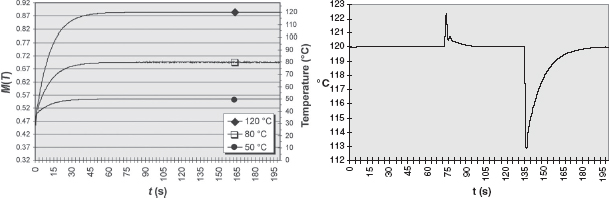
Figure 7.29 (a) Duty-cycle and corresponding temperature reached for different set points for a flow velocity of 10 lh⁻¹; (b) time responses to flow steps of 10 lh⁻¹

7.7 Summary and Future Trends

7.7.1 Summary

In this chapter, two types of smart sensor systems have been considered: those combining discrete types of sensing elements with separated sensor interfaces, and those in which the sensing elements are integrated together with their electronic interfaces on a single chip. In industry, the most commonly used types of sensor elements are:

• platinum resistors and thermistors;
• transistors;
• thermocouples and thermopiles.

The features of these sensing elements have been compared. For on-chip integration, transistors, thermocouples and thermopiles are the most suitable sensing elements.

Besides cost, the main sensor features are:

• (in)accuracy;
• short- and long-term drift;
• noise;
• self-heating;
• dynamic response.

It was shown that it is important to distinguish between accuracy on the one hand and short- and long-term drift on the other as often it suffices both in terms of performance and cost to design for high stability rather than high accuracy. It has been shown that there is a trade-off between noise and resolution on the one hand and measurement time and power dissipation on the other.

Because each temperature sensor measures its own temperature, which can slightly deviate from the object temperature to be measured, it is important to consider the effect of self-heating. This effect depends on power dissipation and on the thermal resistance with respect to the environment. If the sensor is to be switched on only for short periods of time, also the effect of thermal capacitances should be considered.

It has been shown that over the limited temperature range of −55 °C to 150 °C, transistors can very well be used as temperature sensors, especially when low cost, good long-term stability and high sensitivity are required. The base–emitter voltages of transistors provide measures for the temperature and can also be used to generate a (bandgap) reference voltage. These properties are very useful in integrated smart temperature sensors. It has been shown how the differences between the two base–emitter voltages of transistors can be used to generate a voltage that is proportional to the absolute temperature (PTAT).

Various circuit techniques to improve the accuracy of the PTAT voltage have been presented. It has been shown that the implementation of these techniques is not limited to bipolar technology, but that especially in CMOS technology, high-precision circuits can be made.

The principles of a smart temperature sensor with a duty-cycle-modulated output signal have been discussed. The application of smart sensor systems can offer advantages in terms of reliability, accuracy, system simplicity and related cost reduction.

Two case studies for the application of smart temperature sensors were discussed. The first one concerns a measurement system that detects the presence of micro-organisms in food products by monitoring very small temperature differences. In this application, the most important properties of the sensors concern short-term stability, drift, self-heating, reliability and simplicity. The measurement time and absolute accuracy are of less importance. The second case study concerns a very precise and fast control system for stabilizing the temperature of a ceramic substrate. In this application, the thermal time constants must be minimized in order to achieve a fast system response and a highly stable control loop.

7.7.2 Future Trends

The development of mixed-mode analog–digital circuits, such as smart temperature sensors and temperature sensor systems will follow that of the mainstream developments in microelectronics. Therefore an increasing interest has to be expected for the development of sensors which can be implemented in CMOS technology and which can be operated at low supply voltages. To reduce the effects of self-heating and to reduce energy consumption power consumption will be further reduced. The CMOS substrate pnp transistors appear to be rather suited for use as temperature-sensing element [25, 26].

An important way to reduce the sensor-system costs will be found in designing novel sensors that without calibration can offer a high accuracy. Because the piezojunction effect is the main cause of drift it is to be expected that the novel designs will take advantage of recently acquired knowledge concerning minimization of this effect. Again CMOS substrate pnp transistors are rather suited for low-drift design [2, 25, 26].

An on-going discussion in sensor technology is whether or not to integrate the sensing elements together with their interfaces and microcontrollers on the same chips. Often multi-die solutions can simplify design problems as posed by physical constraints. Consequently, systems-in-a-package solutions will often be preferred to systems on a chip. A main problem to be solved concerns the complexity of testing electrophysical systems. Therefore, the development of such smart sensor system will be performed in an overall design approach concerning the overall system features, including long- and short-term accuracy and reliability.

Problems

7.1 Self-heating and thermal capacity (see Section 7.2.6)

An integrated smart temperature sensor has been implemented on a 2 mm×1 mm silicon chip. On both sides, this chip is exposed to laminar airflow of 1 m s⁻¹ (see Figure 7.7(a)). The temperature (≈300 K) of the flowing air is to be measured. The power dissipation P of the sensor amounts to 1 mW. Using the experimental results shown in Figure 7.7(b), answer the following questions:

(1) What is the temperature rise of the sensor chip due to self-heating by its power dissipation of 1 mW?

(2) Suppose that only at one side the chip is exposed to the flow and that the other side is thermally insulated. What would be the temperature rise due to the power dissipation?

(3) Suppose that there is a double-sided flow, as mentioned in (1). To reduce the self-heating effect, the power supply is switched on for only 30 ms. Calculate the mean temperature rise ΔT_mean during this time.

(4) Suppose that the chip thickness was twice that shown in Figure 7.7(a). What would be the consequence for the temperature rise, as calculated in part (3) of this problem?

(5) For a long time the sensor is periodically switched on during t_m = 30 ms at intervals of t_i = 3 s. What is the mean temperature rise time in this case?

7.2 Biasing sensitivities of temperature sensors (Sections 7.3 and 7.4)

Three temperature sensors, a transistor, a thermistor and a Pt100 element (see Figure 7.30) are biased with a current source I_s.

The output voltages V₀ represent the temperature-dependent output signals. The manufacturer's specifications state that for the transistor V_BE (273 K) = 650 mV and for the thermistor the parameter a = 8.6×10⁻⁴ K⁻¹, b = 2.2×10⁻⁴ K⁻¹, c = 0×10⁻⁴ K⁻¹ (see Equation (7.7) for a definition of the parameters a, b and c).

An undesired change in I_s causes an error in V₀ which is equivalent to a temperature error in the sensing elements. Calculate the equivalent temperature errors for a 1% change in I_s for the three sensors at T = 273 K.

7.3 Sampling noise (Sections 7.2.3 and 7.5.1)

A smart temperature sensor generates a duty-cycle modulated output signal (Figure 7.16(c)) with a period t_p = 300 μs. The duty cycle varies linearly with the temperature, which has a sensitivity of 0.5% K⁻¹. This duty cycle is measured by sampling the output signal at time intervals t_s = 0.3 μs.

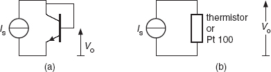
Figure 7.30 Biasing of temperature sensors: (a) a transistor element, (b) resistive elements

Two counters record the number of sampling pulses; one keeps track of the total time and the other the time that the signal is high. Because the sampling moments are not synchronous with the sensor signal, some sampling noise is introduced. The standard deviation of this noise should be less than 0.01 K. Calculate the minimum number N_min of periods of the sensor signal required to measure the temperature.

References

[1] Michalski, L., Eckersdorf, K. and McGhee, J. (1991). Temperature Measurement, John Wiley & Sons, Ltd, Chichester.

[2] Fruett, F. and Meijer, G.C.M. (2002). The Piezojunction Effect in Silicon Integrated Circuits and Sensors, Kluwer, Boston, MA.

[3] Meijer, G.C.M. and van Herwaarden, A.W. (1994). Thermal Sensors, IOP, Bristol.

[4] Meijer, G.C.M. (1982). Integrated circuits and components of bandgap references and temperature transducers, PhD Dissertation, Delft University of Technology.

[5] YSI (1989). Precision Thermistors, Yellow Springs, USA, presently www.meas-spec.com.

[6] Slotboom, J.W. and de Graaf, H.C. (1976). Measurements of bandgap narrowing in Si bipolar transistors, SolidState Electronics, 19, 857–862.

[7] Meijer, G.C.M. and Vingerling, K. (1980). Measurement of the temperature dependence of the I_C–V_BE characteristics of integrated bipolar transistors, IEEE Journal of Solid-State Circuits, 15, 237–241.

[8] Meijer, G.C.M., Schmale, P.C. and van Zalinge, K. (1982). A new curvature-corrected bandgap reference, IEEE Journal of Solid-State Circuits, 17, 1139–1143.

[9] Timko, M.P. (1976). A two-terminal IC temperature transducer, IEEE Journal of Solid-State Circuits, SC-11, 784–788.

[10] Meijer, G.C.M. (1978). A new configuration for temperature transducers and bandgap references. In ESSCIRC 1978, Amsterdam, The Netherlands.

[11] Dobkin, R.C. (1975). Input supply independent circuits, US Patent No. 3930172.

[12] Meijer, G.C.M. (1995). Schakeling voor het opwekken van een temperatuursignaal met een gedefinieerde afhankelijkheid van de temperatuur, Dutch Patent Application No. 1000222.

[13] Meijer, G.C.M., van Gelder, R., Nooder, V., van Drecht, J. and Kerkvliet, H.M.M. (1989). A three-terminal integrated temperature transducer with microcomputer interfacing, Sensors and Actuators A, 18, 195–206.

[14] Smartec (2006-2). “http://www.smartec.nl” www.smartec.nl, data sheet: Universal Transducer Interface UTI.

[15] Melexis (2004). “http://www.melexis.com” www.melexis.com, data sheet: Programmable Sensor Interface MLX90314AB.

[16] Triad Semiconductor (2004). “http://www.triadsemi.com” www.triadsemi.com, data sheet: TASIC002- Smart Sensor ASIC solution on VCA-4.

[17] Analog devices (2004). www.analog.com, data sheet: LC²MOS signal conditioning ADC with RTD current source.

[18] Maxim (2004). www.maxim.com, data sheet: ow-cost precision sensor signal conditioner.

[19] Meijer, G.C.M., Kerkvliet, H.M.M. and Toth, F.N. (1994). Non-invasive detection of microorganisms using smart temperature sensors, Sensors and Actuators B – Chemical, 18, 276–281.

[20] Smartec (2006-1). “http://www.smartec.nl” www.smartec.nl, data sheet: Temperature sensors.

[21] Nieuwenhuizen, M.S. and Venema, A. (1989). Surface acoustic wave chemical sensors, Sensors and Materials, 5, 261.

[22] Vellekoop, M.J. (1994). A smart Lamb-wave sensor system, PhD Dissertation, Delft University of Technology.

[23] van der Meer, P.R., Meijer, G.C.M., Vellekoop, M.J., Kerkvliet, H.M.M. and van den Boom, T.J.J. (1998). A temperature-controlled smart surface-acoustic-wave gas sensor, Sensors and Actuators A – Physical, 71, 27–34.

[24] Mayuresh, V., Kothare, P.J.C., Manfred, M. and Carl, N.N. (1994). A unified framework for the study of anti-windup designs, Automatica, 30.

[25] Wang, G. (2005). CMOS bandgap references and temperature sensors and their applications, PhD Dissertation, Delft University of Technology.

[26] Pertijs, M.A.P., Meijer, G.C.M. and Huijsing, J.H. (2004). Precision temperature measurement using CMOS substrate pnp transistors, Sensors Journal, IEEE, 4, 294.