Part IX
Tests on Contingency Tables
Contingency tables are frequently used to present the outcome of a sample of categorical random variables. These variables can also be the result of categorizing the output of continuous random variables. Of interest are, for example, homogeneity or independence between the variables. We focus on two-dimensional tables, where the categories of one variable define the rows and the categories of another variable the columns. Each cell then contains the frequency of occurrence of the row/column combination in the sample. The simplest case is a ![]() table:
table:

Here we have two binary random variables ![]() and
and ![]() with marginal binomial distribution, or two random variables which are dichotomized into two outcome groups, with labels
with marginal binomial distribution, or two random variables which are dichotomized into two outcome groups, with labels ![]() and
and ![]() . Usually the absolute counts are listed, so
. Usually the absolute counts are listed, so ![]() is the count of outcome
is the count of outcome ![]() of random variable
of random variable ![]() and outcome
and outcome ![]() of random variable
of random variable ![]() , whereas
, whereas ![]() usually denotes the (marginal) sum of the counts of the first column. Instead of absolute counts in a contingency table sometimes relative counts are reported. If not stated otherwise, we work with absolute counts.
usually denotes the (marginal) sum of the counts of the first column. Instead of absolute counts in a contingency table sometimes relative counts are reported. If not stated otherwise, we work with absolute counts.
Extending this notation to ![]() and
and ![]() possible outcomes of
possible outcomes of ![]() and
and ![]() , respectively, we get:
, respectively, we get:
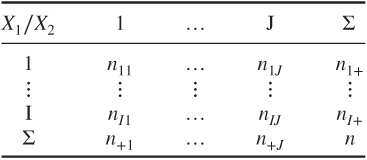
While setting up tests we formulate a test statistic as a function of the random sample to be observed. For this purpose we further denote the random variable withoutput ![]() by
by ![]() ,
, ![]() ,
, ![]() . Concerning distributional assumptions for contingency tables commonly three different sampling distributions are distinguished for the
. Concerning distributional assumptions for contingency tables commonly three different sampling distributions are distinguished for the ![]() 's, depending on the employed sampling scheme. If the sample size is not known beforehand, for example, if observations are taken over a specific period of time, it is assumed that each
's, depending on the employed sampling scheme. If the sample size is not known beforehand, for example, if observations are taken over a specific period of time, it is assumed that each ![]() follows an independent Poisson distribution. For fixed sample sizes
follows an independent Poisson distribution. For fixed sample sizes ![]() we get a multinomial distribution characterized by
we get a multinomial distribution characterized by ![]() and the cell probabilities
and the cell probabilities ![]() . In experimental studies the total number of individuals in each group is also often fixed and the resulting sample distribution is a product of independent multinomial distributions. Throughout Chapter 14 we use the above notation.
. In experimental studies the total number of individuals in each group is also often fixed and the resulting sample distribution is a product of independent multinomial distributions. Throughout Chapter 14 we use the above notation.