Chapter 17
Tests in variance analysis
Analysis of variance (ANOVA) in its simplest form analyzes if the mean of a Gaussian random variable differs in a number of groups. Often the factor which determines each group is given by applying different treatments to subjects, for example, in designed experiments in technical applications or in clinical studies. The problem can thereby be seen as comparing group means, which extends the t-test to more than two groups. The underlying statistical model may also be presented as a special case of a linear model. In Section 17.1 we handle the one- and two-way cases of ANOVA. The two-way case extends the treated problem to groups characterized by two factors. In this case it is also of interest if the two factors influence each other in their effect on the measured variable, and hence show an interaction effect. One of the crucial assumptions of an ANOVA is the homogeneity of variance within all groups. Section 17.2 deals with tests to check this assumption.
17.1 Analysis of variance
17.1.1 One-way ANOVA
| Description: |
Tests if the mean of a Gaussian random variable is the same in  groups. groups. |
| Assumptions: |
- Let
 , ,  , be , be  independent samples of independent Gaussian random variables with the same variance but possibly different group means. independent samples of independent Gaussian random variables with the same variance but possibly different group means.
- The sample sizes of the
 samples are samples are  with with  . .
- The random variables
 can be modeled as can be modeled as  with with  , ,  . .
|
| Hypotheses: |
 vs vs  for at least one for at least one  . . |
| Test statistic: |
|
|
 |
|
 |
| Test decision: |
Reject  if for the observed value if for the observed value  of of  |
|
 |
| p-values: |
 |
| Annotations: |
- The test statistic
 is is  -distributed (Rencher 1998, chapter 4). -distributed (Rencher 1998, chapter 4).
 is the is the  -quantile of the F-distribution with -quantile of the F-distribution with  and and  degrees of freedom. degrees of freedom.- The numerator of the test statistic is also called MST (mean sum of squares for treatment) and the denominator MSE (mean sum of squares of errors).
- Note that we have presented the one-way model and test for the more general case of an unbalanced design where the sample sizes in the different groups may vary. A balanced design is characterized by an equal number of observations in each group.
|
Example
To test if the means of the harvest in kilograms of tomatoes in three different greenhouses differ. The dataset contains observations from five fields in each greenhouse (dataset in
Table A.12).
SAS code
proc anova data = crop;
 class house
 model kg = house;
run;
quit;
SAS output
Source    DF     Anova SS   Mean Square  F Value   Pr> F
house      2   0.16329333    0.08164667     0.33   0.7262
Remarks:
R code
summary(aov(crop$kg∼factor(crop$house)))
R output
                   Df Sum Sq Mean Sq F value Pr(>F)
factor(crop$house)  2 0.1633 0.08165   0.329  0.726
Residuals          12 2.9815 0.24846
Remarks:
- The function aov() performs an analysis of variance in R. The response variable is placed on the left-hand side of the
 symbol and the independent variables which define the groups on the right-hand side.
- We use the R function factor() to tell R that house is a categorical variable.
- The summary function gets R to return the sum of squares, degrees of freedom, p-values, etc.
17.1.2 Two-way ANOVA
| Description: |
Tests if the mean of a Gaussian random variable is the same in groups defined by two factors of interest. |
| Assumptions: |
- Let
 , ,  , ,  , ,  describe a sample of size describe a sample of size  of independent Gaussian random variables. of independent Gaussian random variables.
- In each of the
 groups defined by the two factors, we have an equal number of groups defined by the two factors, we have an equal number of  observations (balanced design). observations (balanced design).
|
|
- Each of the variables
 can be modeled as can be modeled as with with  , where , where  is the overall mean and is the overall mean and  and and  are the deviations from it for the first and the second factor and are the deviations from it for the first and the second factor and  describes the interaction between them. describes the interaction between them.
|
| Hypotheses: |
(A)  |
|
vs  for at least one pair for at least one pair  |
|
(B)  |
|
vs  for at least one for at least one  |
|
(C)  |
|
vs  for at least one for at least one  |
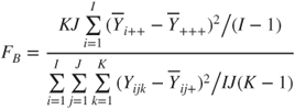
| Test statistic: |
|
|
(A)  |
|
(B)  |
|
(C)  |
|
with |
|
 |
|
 |
| Test decision: |
Reject  if for the observed value if for the observed value  of of  , ,  or or  |
|
(A)  |
|
(B)  |
|
(C)  |
| p-values: |
 |
| Annotations: |
- The test statistic
 is F-distributed with is F-distributed with  (A), (A),  (B) or (B) or  degrees of freedom for the nominator and degrees of freedom for the nominator and  degrees of freedom for the denominator (Montgomery and Runger 2007, chapter 14). degrees of freedom for the denominator (Montgomery and Runger 2007, chapter 14).
|
|
 is the is the  -quantile of the F-distribution with -quantile of the F-distribution with  and and  degrees of freedom. degrees of freedom.- Hypothesis (A) tests if there is an interaction between the two factors. Hypotheses (A) and (B) are testing the main effects of the two factors.
|
Example
To test if the means of the harvest in kilograms of tomatoes in three different greenhouses and using five different fertilizers differ. The dataset contains observations from five fields with each fertilizer in each greenhouse (dataset in
Table A.12).
SAS code
proc anova data= crop;
      class house fertilizer;
      model kg =  house fertilizer;
run;
quit;
SAS output
                    The ANOVA Procedure
Dependent Variable: kg
Source       DF    Anova SS  Mean Square  F Value  Pr> F
house         2  0.16329333   0.08164667     0.50  0.6268
fertilizer    4  1.66337333   0.41584333     2.52  0.1235
Remarks:
R code
kg<-crop$kg
field<-crop$house
fertilizer<-crop$fertilizer
summary(aov(kg∼factor(field)+factor(fertilizer)))
R output
                   Df Sum Sq Mean Sq F value Pr(>F)
factor(house)       2 0.1633  0.0816   0.496  0.627
factor(fertilizer)  4 1.6634  0.4158   2.524  0.123
Residuals           8 1.3181  0.1648
Remarks:
- The function aov() performs an ANOVA in R. The response variable is placed on the left-hand side of the
 symbol and the independent variables which define the groups on the right-hand side separated by a plus (+). To incorporate an interaction term a star is used, for example, variable1
 variable2.
- We use the R function factor() to tell R that house is a categorical variable.
- The summary function gets R to return the sum of squares, degrees of freedom, p-values, etc.
17.2 Tests for homogeneity of variances
17.2.1 Bartlett test
| Description: |
Tests if the variances of  Gaussian populations differ from each other. Gaussian populations differ from each other. |
| Assumptions: |
- Data are measured on an interval or ratio scale.
- Data are randomly sampled from
 independent Gaussian distributions. independent Gaussian distributions.
- The
 random variables random variables  from where the samples are drawn have variances from where the samples are drawn have variances  . .
- Further
 is the is the  sample with sample with  observations, observations,  . .
|
| Hypotheses: |
 vs vs  for at least one for at least one  |
| Test statistic: |
|
|
 |
|
with  , ,  |
|
and  |
| Test decision: |
Reject  if for the observed value if for the observed value  of of  |
|
 |
| p-values: |
 |
| Annotations: |
- The test statistic
 is is  -distributed (Glaser 1976). -distributed (Glaser 1976).
 is the is the  -quantile of the -quantile of the  -distribution with -distribution with  degrees of freedom. degrees of freedom.- This test was introduced by Maurice Bartlett (1937).
- The Bartlett test is very sensitive to the violation of the Gaussian assumption. If the samples are not Gaussian distributed an alternative is Levene's test (Test 17.2.2).
|
Example
To test if the variances of the harvest in kilograms of tomatoes in three different greenhouses are the same (dataset in
Table A.12).
SAS code
proc glm data = crop;
 class house;
 model kg = house;
 means house /hovtest=BARTLETT ;
run;
quit;
SAS output
                The GLM Procedure
 Bartlett's Test for Homogeneity of kg Variance
  Source        DF    Chi-Square    Pr > ChiSq
  house          2        2.1346        0.3439
Remarks:
- The SAS procedure proc glm provides the Bartlett test.
- The first lines of code are enabling an ANOVA (see Test 16.2.1).
- The code means house /hovtest=BARTLETT lets SAS conduct the Bartlett test.
R code
bartlett.test(crop$kg∼crop$house)
R output
 Bartlett test of homogeneity of variances
data:  crop$kg by crop$field
Bartlett's K-squared = 2.1346, df = 2, p-value = 0.3439
Remarks:
- The function bartlett.test() conducts the Bartlett test.
- The analysis variable is coded on the left-hand side of the
 and the group variable on the right-hand side.
17.2.2 Levene test
| Description: |
Tests if the variances of k populations differ from each other. |
| Assumptions: |
- Data are measured on an interval or ratio scale.
- Data are randomly sampled from
 independent random variables independent random variables  with variances with variances  . .
- Further
 is the is the  sample with sample with  observations, observations,  . .
|
| Hypotheses: |
 vs vs  for at least one for at least one  . . |
| Test statistic: |
|
|
 |
|
 |
| Test decision: |
Reject  if for the observed value if for the observed value  of of  |
|
 |
| p-values: |
 |
| Annotations: |
- The test statistic
 is is  -distributed. -distributed.
 is the is the  -quantile of the F-distribution with -quantile of the F-distribution with  and and  degrees of freedom. degrees of freedom.- This test was introduced by Howard Levene 1960. In 1974 Morton Brown and Alan Forsythe proposed the use of the median or trimmed mean instead of the mean for calculating the
 (Brown and Forsythe 1974). This test is called the Brown–Forsythe test. (Brown and Forsythe 1974). This test is called the Brown–Forsythe test.
- This test does not need the assumption of underlying Gaussian distributions and should be used if that assumption is doubtful. If the data are Gaussian distributed Bartlett's test can be used (see Test 17.2.1).
|
Example
To test if the variances of the harvest in kilograms of tomatoes in three different greenhouses are the same (dataset in
Table A.12).
SAS code
proc glm data = crop;
 class house;
 model kg = house;
 means house /hovtest=levene (TYPE=ABS) ;
run;
quit;
SAS output
      Levene's Test for Homogeneity of kg Variance
      ANOVA of Absolute Deviations from Group Means
                  Sum of        Mean
Source     DF     Squares      Square    F Value    Pr> F
house       2      0.2675      0.1337       2.79    0.1012
Error      12      0.5753      0.0479
Remarks:
- The SAS procedure proc glm provides the Levene test.
- The first lines of code are enabling an ANOVA (see Test 16.2.1).
- The code means house /hovtest=levene (TYPE=ABS) lets SAS do the Levene test. In SAS it is also possible to choose the option (TYPE=SQUARE) which uses the squared differences.
- The Brown–Forsythe test can be conducted with the option /hovtest=BF.
R code
# Calculate group means for each field
m<-tapply(crop$kg,crop$house,mean)
# Calculate the Z's
z<-abs(crop$kg-m[crop$house])
# Overall mean of the Z's
z_mean=mean(z)
# Group mean of the Z's
z_gm<-tapply(z,crop$house,mean)
# Make a matrix of the Z's (group in the rows)
z_matrix<-rbind(z[crop$house==1],z[crop$house==2],
                z[crop$house==3])
# Calculate the numerator
nu<-0
for (i in 1:3)
 {
  u<-5*(z_gm[i]-z_mean)∧2
  nu<-nu+u
 }
# Calculate the denominator
de<-0
for (j in 1:3)
{
 for (i in 1:5)
  {
   e<-(z_matrix[j,i]-z_gm[j])∧2
   de<-de+e
  }
}
# Calculate test statistic and p-value
l<-(12*nu)/(2*de)
p_value<-1-pf(l,2,12)
# Output results
“Levene Test”
l
p_value
R output
[1] “Levene Test”
> l
       1
2.789499
> p_value
        1
0.1011865
>
Remarks:
- There is no basic R function to calculate Levene's test directly.
- In this example we have
 and
and  . The respective parts must be adopted if other data are used.
- To apply the Brown–Forsythe test just change the first line of code to m<-tapply(crop$kg,crop$house,median).
References
Bartlett M.S. Properties of sufficiency and statistical tests. Proceedings of the Royal Statistical Society Series A 160, 268–282.
Brown M.B. and Forsythe A.B. 1974 Robust tests for the equality of variances. Journal of the American Statistical Association 69, 364–367.
Glaser R.E. 1976 Exact critical values for Bartletts test for homogeneity of variances. Journal of the American Statistical Association 71, 488–490.
Levene H. 1960. Contributions to Probability and Statistics: Essays in Honor of Harold Hotelling (eds Olkin I et al.), pp. 278–292. Stanford University Press.
Montgomery D.C. and Runger G.C. 2007 Applied Statistics and Probability for Engineers, 4th edn. John Wiley & Sons, Ltd.
Rencher A.C. 1998 Multivariate Statistical Inference and Applications. John Wiley & Sons, Ltd.


 symbol and the independent variables which define the groups on the right-hand side.


 variable2.
 symbol and the independent variables which define the groups on the right-hand side separated by a plus (+). To incorporate an interaction term a star is used, for example, variable1
 variable2.
 and the group variable on the right-hand side.
 and
and  . The respective parts must be adopted if other data are used.