2.5Robust preferences on asset profiles

In this section, we discuss the structure of preferences for assets on a more fundamental level. Instead of assuming that the distributions of assets are known and that preferences are defined on a set of probability measures, we will take as our basic objects the assets themselves. An asset will be viewed as a function which associates real-valued payoffs to possible scenarios. More precisely, X will denote a set of bounded measurable functions X on some measurable set (Ω,F). We emphasize that no a priori probability measure is given on (Ω,F). In other words, we are facing uncertainty instead of risk.

We assume that X is endowed with a preference relation . In view of the financial interpretation, it is natural to assume that is monotone in the sense that

Under a suitable condition of continuity, we could apply the results of Section 2.1 to obtain a numerical representation of . L. J. Savage introduced a set of additional axioms which guarantee that there is a numerical representation of the special form

where Q is a probability measure on (Ω,F) and u is a function on ℝ. The measure Q specifies the subjective view of the probabilities of events which is implicit in the preference relation . Note that the function u : ℝ → ℝ is determined by restricting U to the class of constant functions on (Ω,F). Clearly, the monotonicity of is equivalent to the condition that u is an increasing function.

Definition 2.70. A numerical representation of the form (2.29) will be called a Savage representation of the preference relation .

◊

Remark 2.71. Let μQ,X denote the distribution of X under the subjective measure Q. Clearly, the preference order on X given by (2.29) induces a preference order on

with von Neumann–Morgenstern representation

i.e.,

On this level, Section 2.3 specifies the conditions on UQ which guarantee that u is a (strictly concave and strictly increasing) utility function.

◊

Remark 2.72. Even if an economic agent with preferences accepts the view that scenarios ω ∈ Ω are generated in accordance to a given objective probability measure P on (Ω,F), the preference order on X may be such that the subjective measure Q appearing in the Savage representation (2.29) is different from the objective measure P. Suppose, for example, that P is Lebesgue measure restricted to Ω = [0, 1], and that X is the space of bounded right-continuous increasing functions on [0, 1]. Let μP,X denote the distribution of X under P. By Lemma A.23, every probability measure on ℝ with bounded support is of the form μP,X for some X ∈ X , i.e.,

Suppose the agent agrees that, objectively, X ∈ X can be identified with the lottery μP,X, so that the preference relation on X could be viewed as a preference relation on Mb(ℝ) with numerical representation

This does not imply that U∗ satisfies the assumptions of Section 2.2; in particular, the preference relation on Mb(ℝ) may violate the independence axiom. In fact, the agent might take a pessimistic view and distort P by putting more emphasis on unfavorable scenarios. For example, the agent could replace P by the subjective measure

for some α ∈ (0, 1) and specify preferences by a Savage representation in terms of u and Q. In this case,

Note that X(0) = (μP,X) for

where supp μ is the support of μ. Hence, replacing P by Q corresponds to a nonlinear distortion on the level of lotteries: μ = μP,X is distorted to the lottery μ∗ = μQ,X given by

and the preference relation on lotteries has the numerical representation

Let us now show that such a subjective distortion of objective lotteries provides a possible explanation of the Allais paradox. Consider the lotteries μi and νi, i = 1,2, described in Example 2.30. Clearly,

while

For the particular choice u(x) = x we have U∗(ν2) > U∗(μ2), and for α > 9/2409 we obtain U∗(μ1) > U∗(ν1), in accordance with the observed preferences ν2 μ2 and μ1 ν1 described in Example 2.30.

For a systematic discussion of preferences described in terms of a subjective distortion of lotteries we refer to [179]. In Section 4.6, we will discuss the role of distortions in the context of risk measures, and in particular the connection to Yaari’s “dual theory of choice under risk” [276].

◊

Even in its general form (2.29), however, the paradigm of expected utility has a limited scope as illustrated by the following example.

Example 2.73 (Ellsberg paradox). You are faced with a choice between two urns, each containing 100 balls which are either red or black. In the first urn, the proportion p of red balls is know; assume, e.g., p = 0.49. In the second urn, the proportion is unknown. Suppose that you get 1000€ if you draw a red ball and 0€ otherwise. In this case, most people would choose the first urn. Naturally, they make the same choice if you get 1000€ for drawing a black ball and 0€ for a red one. But this behavior is not compatible with Savage’s paradigm of subjective expected utility: For any subjective probability of drawing a red ball in the second urn, the first choice would imply p > , the second would yield 1 − p > 1 − , and this is a contradiction.

◊

For this reason, we are going to make one further conceptual step beyond the Savage representation before we start to prove a representation theorem for preferences on X . Instead of a single measure Q, let us consider a whole class Q of measures on (Ω,F). Our aim is to characterize those preference relations on X which admit a representation of the form

This may be viewed as a robust version of the paradigm of expected utility: The agent has in mind a whole collection of possible probabilistic views of the given set of scenarios and takes a worst-case approach in evaluating the expected utility of a given payoff.

It will be convenient to extend the discussion to the following framework where payoffs can be lotteries. Let X denote the space of all bounded measurable functions on (Ω,F). We are going to embed X into a certain space of functions on (Ω,F) with values in the convex set

of boundedly supported Borel probability measures on ℝ. More precisely, is defined as the convex set of all those stochastic kernels (ω, dy) from (Ω,F) to ℝ for which there exists a constant c ≥ 0 such that

In economics, the elements of are sometimes called acts; see, for example, [193]. The space X can be embedded into by virtue of the mapping

In this way, X can be identified with the set of all ∈ for which the measure (ω, ·) is a Dirac measure. A preference order on X defined by (2.30) clearly extends to by

where is the affine function on Mb(ℝ) defined by

Remark 2.74. Restricting the preference order on obtained from (2.32) to the constant maps (ω) = μ for μ ∈ Mb(ℝ), we obtain a preference order on Mb(ℝ), and on this level we know how to characterize risk aversion by the property that u is strictly concave.

◊

Example 2.75. Let us show how the Ellsberg paradox fits into our extended setting, and how it can be resolved by a suitable choice of the set Q. For Ω = {0, 1} define

and

Take

with [a, b] ⊂ [0, 1]. For any increasing function u, the functional

satisfies

as soon as a < p < b, in accordance with the preferences described in Example 2.73.

◊

Let us now formulate those properties of a preference order on the convex set which are crucial for a representation of the form (2.32). For , ∈ and α ∈ (0, 1), (2.32) implies

In contrast to the Savage case Q = {Q}, we can no longer expect equality, except for the case of certainty (ω) ≡ μ. If ∼ , then () = (), and the lower bound reduces to () = (). Thus, satisfies the following two properties:

Uncertainty aversion: If , ∈ are such that ∼ , then

Certainty independence: For , ∈ , ≡ μ ∈ Mb(ℝ), and α ∈ (0, 1] we have

Remark 2.76. In order to motivate the term “uncertainty aversion”, consider the situation of Example 2.75. Suppose that an agent is indifferent between the choices 0 and 1, which both involve the same kind of Knightian uncertainty. For α ∈ (0, 1), the convex combination := α0 +(1−α)1,which is weakly preferred to both 0 and 1 in the case of uncertainty aversion, takes the form

i.e., uncertainty is reduced in favor of risk. For α = 1/2, the resulting lottery (ω) ≡ (δ1000+ δ0) is independent of the scenario ω, i.e., Knightian uncertainty is completely replaced by the risk of a coin toss.

◊

Remark 2.77. The axiom of “certainty independence” extends the independence axiom for preferences on lotteries to our present setting, but only under the restriction that one of the two contingent lotteries and Y is certain, i.e., does not depend on the scenario ω ∈ Ω. Without this restriction, the extended independence axiom would lead to the Savage representation in its original form (2.29); see Exercise 2.5.3 below. There are good reasons for not requiring full independence for all ∈ . As an example, take Ω = {0, 1} and define (ω) = δω, (ω) = δ1−ω, and = . An agent may prefer over , thus expressing the implicit view that scenario 1 is somewhat more likely than scenario 0. At the same time, the agent may like the idea of hedging against the occurrence of scenario 0, and this could mean that the certain lottery

is preferred over the contingent lottery

thus violating the independence assumption in its unrestricted form. In general, the role of as a hedge against scenarios unfavorable for requires that and are not comonotone, i.e.,

Thus, the wish to hedge would still be compatible with the following enforcement of certainty independence, called

Comonotonic independence: For , , ∈ and α ∈ (0, 1]

whenever and are comonotone in the sense that (2.33) does not occur.

The consequences of requiring comonotonic independence will be analyzed in Exercise 2.5.4 below. It is also relevant to weaken the axiom of certainty independence and to require instead

Weak certainty independence: if for , ∈ and for some ν ∈ Mb(S) and α ∈ (0, 1] we have α+ (1 − α)ν α + (1 − α)ν, then

The consequences of requiring weak certainty independence will be analyzed in Theorem 2.88 below.

◊

From now on, we assume that is a given preference order on . The set Mb(ℝ) will be regarded as a subset of by identifying a constant function ≡ μ with its value μ ∈ Mb(ℝ). We assume that possesses the following properties:

–Uncertainty aversion.

–Certainty independence.

–Monotonicity: If (ω) (ω) for all ω ∈ Ω, then . Moreover, is compatible with the usual order on ℝ, i.e., δy δx if and only if y > x.

–Continuity: The following analogue of the Archimedean axiom holds on : If , , ∈ are such that , then there are α, β ∈ (0, 1) with

Moreover, for all c > 0 the restriction of to M1([−c, c]) is continuous with respect to the weak topology.

Let us denote by

the class of all set functions Q : F → [0, 1] which are normalized to Q[ Ω ] = 1 and which are finitely additive, i.e., Q[ A ∪ B ] = Q[ A ] + Q[ B ] for all disjoint A, B ∈ F; see Appendix A.6. By EQ[ X ] we denote the integral of X with respect to Q ∈ M1,f ; see Appendix A.6. With M1 = M1(Ω,F) we denote the σ-additive members of M1,f , that is, the class of all probability measures on (Ω,F). Note that the inclusion M1 ⊂ M1,f is typically strict as is illustrated by Example A.56.

Theorem 2.78. Consider a preference order on satisfying the four properties of uncertainty aversion, certainty independence, monotonicity, and continuity.

(a) There exists a strictly increasing function u ∈ C(ℝ) and a convex set Q ⊂ M1,f (Ω,F) such that

is a numerical representation of . Moreover, u is unique up to positive affine transformations.

(b) If the induced preference order on X , viewed as a subset of as in (2.31), satisfies the following additional continuity property

then the set functions in Q are in fact probability measures, i.e., each Q ∈ Q is σ-additive. In this case, the induced preference order on X has the robust Savage representation

with Q ⊂ M1(Ω,F).

Remark 2.79. Even without its axiomatic foundation, the robust Savage representation is highly plausible as it stands, since it may be viewed as a worst-case approach to the problem of model uncertainty. This aspect will be of particular relevance in our discussion of risk measures in Chapter 4.

◊

The proof of Theorem 2.78 needs some preparation.

When restricted to Mb(ℝ), viewed as a subset of , the axiom of certainty independence is just the independence axiom of the von Neumann–Morgenstern theory. Thus, the preference relation on Mb(ℝ) satisfies the assumptions of Corollary 2.28, and we obtain the existence of a continuous function u : ℝ → ℝ such that

is a numerical representation of on the set Mb(ℝ). Moreover, u is unique up to positive affine transformations. The second part of our monotonicity assumption implies that u is strictly increasing. Without loss of generality, we assume u(0) = 0 and u(1) = 1.

Remark 2.80. In view of the representation (2.36), it follows as in (2.11) that any μ ∈ Mb(ℝ) admits a unique certainty equivalent c(μ) ∈ ℝ for which

Thus, if X ∈ X is defined for ∈ as X(ω) := c(ω), then the first part of our monotonicity assumption yields

and so the preference relation on is uniquely determined by its restriction to X .

◊

Lemma 2.81. There exists a unique extension of the functional in (2.36) as a numerical representation of on .

Proof. For ∈ let c > 0 be such that (ω, [−c, c]) = 1 for all ω ∈ Ω. Then

and our monotonicity assumption implies that

We will show below that there exists a unique α ∈ [0, 1] such that

Once this has been achieved, the only possible choice for () is

This definition of a numerical representation of on .

The proof of the existence of a unique α ∈ [0, 1] with (2.38) is similar to the proof of Lemma 2.24. Uniqueness follows from the monotonicity

which is an immediate consequence of the von Neumann–Morgenstern representation (2.36). Now we let

We have to exclude the two following cases:

In the case (2.40), our continuity axiom yields some β ∈ (0, 1) for which

where γ = βα + (1 − β) > α, in contradiction to the definition of α.

If (2.41) holds, then the same argument as above yields β ∈ (0, 1) with

By our definition of α there must be some γ ∈ (βα, α) with

where the second relation follows from (2.39). This, however, is a contradiction.

Remark 2.82. Note that the proof of the preceding lemma relies only on the assumptions of continuity and monotonicity of . Certainty independence and uncertainty aversion are not needed.

◊

Via the embedding (2.31), Lemma 2.81 induces a numerical representation U of on X given by

The following proposition clarifies the properties of the functional U and provides the key to a robust Savage representation of the preference order on X .

Proposition 2.83. Given u of (2.36) and the numerical representation U on X constructed via Lemma 2.81 and (2.42), there exists a unique functional ϕ : X → ℝ such that

and such that the following four properties are satisfied:

–Monotonicity: If Y(ω) ≥ X(ω) for all ω, then ϕ(Y) ≥ ϕ(X).

–Concavity: If λ ∈ [0, 1] then ϕλX + (1 − λ)Y≥ λϕ(X) + (1 − λ)ϕ(Y).

–Positive homogeneity: ϕ(λX) = λϕ(X) for λ ≥ 0.

–Cash invariance: ϕ(X + z) = ϕ(X) + z for all z ∈ ℝ.

Proof. Denote by Xu the space of all X ∈ X which take values in a compact subset of the range u(ℝ) of u. Clearly, Xu coincides with the range of the nonlinear transformation Note that this transformation is bijective since u is continuous and strictly increasing due to our assumption of monotonicity. Thus, ϕ is well-defined on Xu via (2.43). We show next that this ϕ has the four properties of the assertion.

Monotonicity is obvious. For positive homogeneity on Xu, it suffices to show that ϕ(λX) = λϕ(X) for X ∈ Xu and λ ∈ (0, 1]. Let X0 ∈ X be such that u(X0) = X. We define ∈ by

By (2.37), ∼ δZ where Z is given by

where we have used our convention u(0) = 0. It follows that u(Z) = λu(X0) = λX, and so

As in (2.38), one can find ν ∈ Mb(ℝ) such that ν ∼ δX0 . Certainty independence implies that

Indeed, ν ∼ δX0 is equivalent to ν δX0 and ν ≺ δX0 , and so certainty independence implies that we can have neither λν + (1 − λ)δ0 nor ≺ λν + (1 − λ)δ0. Hence,

This shows that ϕ is positively homogeneous on Xu.

Since the range of u is an interval, we can extend ϕ from Xu to all of X by positive homogeneity, and this extension, again denoted ϕ, is also monotone and positively homogeneous.

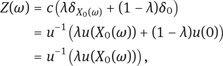
Let us now show that ϕ is cash invariant. First note that

for any x such that u(x) ≠ 0. Now take X ∈ X and z ∈ ℝ. By positive homogeneity, we may assume without loss of generality that 2X ∈ Xu and 2z ∈ u(ℝ). Then there are X0 ∈ X such that 2X = u(X0) as well as z0, x0 ∈ ℝ with 2z = u(z0) and 2ϕ(X) = u(x0). Note that δX0 ∼ δx0 . Thus, as above, certainty independence yields

On the one hand, it follows that

On the other hand, the same reasoning which lead to (2.44) shows that

As to concavity, we need only show that Xu, by Exercise 2.5.2 below. Let X0, Y0 ∈ X be such that X = u(X0) and Y = u(Y0). If ϕ(X) = ϕ(Y), then δX0 ∼ δY0 , and uncertainty aversion gives

which by the same arguments as above yields

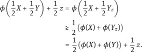
The case in which ϕ(X) > ϕ(Y) can be reduced to the previous one by letting and by replacing Y by Yz := Y + z. Cash invariance then implies that

A functional ϕ : X → ℝ satisfying the properties of monotonicity, concavity, positive homogeneity, and cash invariance is sometimes called a coherent monetary utility functional. The functional ρ(X) := −ϕ(X) is called a coherent risk measure. Functionals of this type will be studied in detail in Chapter 4.

Exercise 2.5.1. Let ϕ : X → ℝ be a functional that satisfies the properties of monotonicity and cash invariance stated in Proposition 2.83. Show that is Lipschitz continuous on X with respect to the supremum norm · , i.e.,

◊

Exercise 2.5.2. Suppose that ϕ : X → ℝ is monotone, cash invariant, and satisfies for all X, Y ∈ X . Use Exercise 2.5.1 to show that ϕ is concave.

◊

Let us now show that a function with the four properties established in Proposition 2.83 can be represented in terms of a family of set functions in the class M1,f .

Proposition 2.84. A functional ϕ : X → ℝ is monotone, concave, positively homogeneous, and cash invariant if and only if there exists a set Q ⊂ M1,f such that

Moreover, the set Q can always be chosen to be convex and such that the infimum above is attained, i.e.,

Proof. The necessity of the four properties is obvious. Conversely, we will construct for any X ∈ X a finitely additive set function Q X such that ϕ(X) = EQX [ X ] and ϕ(Y) ≤ EQX [ Y ] for all Y ∈ X . Then

where Q0 := {QX | X ∈ X }. Clearly, (2.45) remains true if we replace Q0 by its convex hull Q := conv Q0.

To construct QX for a given X ∈ X , we define three convex sets in X by

The convexity of C1 and C2 implies that the convex hull of their union is given by

Since Y ∈ C is of the form Y = αY1 + (1 − α)Y2 for some Yi ∈ Ci and α ∈ [0, 1],

and so B and C are disjoint. Let X be endowed with the supremum norm Y:= supω∈Ω |Y(ω)|. Then C1, and hence C , contains the unit ball in X . In particular, C has nonempty interior. Thus, we may apply the separation argument in the form of Theorem A.58, which yields a nonzero continuous linear functional on X such that

Since C contains the unit ball, c must be strictly positive, and there is no loss of generality in assuming c = 1. In particular, (1) ≤ 1 as 1 ∈ C . On the other hand, any constant b > 1 is contained in B, and so

Hence, (1) = 1.

If A ∈ F then Ac ∈ C1 ⊂ C , which implies that

By Theorem A.54 there exists a finitely additive set function Q X ∈ M1,f (Ω,F) such that (Y) = EQX [ Y ] for any Y ∈ X .

It remains to show that EQX [ Y ]≥ ϕ(Y) for all Y ∈ X , with equality for Y = X. By the cash invariance of ϕ, we need only consider the case in which ϕ(Y) > 0. Then

and Yn → Y/ϕ(Y) uniformly, whence

On the other hand, X /ϕ(X) ∈ C2 ⊂ C yields the inequality

We are now ready to complete the proof of the first main result in this section.

Proof of Theorem 2.78. (a): By Remark 2.80, it suffices to consider the induced preference relation on X once the function u has been determined. According to Lemma 2.81 and the two Propositions 2.83 and 2.84, there exists a convex set Q ⊂ M1,f such that

is a numerical representation of on X . This proves the first part of the assertion.

(b): The assumption (2.35) applied to X ≡ 1 and Y ≡ b < 1 gives that any sequence with X n ↗ 1 is such that X n b for large enough n. We claim that this implies that U(Xn) ↗ u(1) = 1. Otherwise, U(Xn)would increase to some number a < 1. Since u is continuous and strictly increasing, we may take b such that a < u(b) < 1. But then U(Xn) > U(b) = u(b) > a for large enough n, which is a contradiction.

In particular, we obtain that for any increasing sequence of events An ∈ F with

But this means that each Q ∈ Q satisfies limn Q[ An ] = 1, which is equivalent to the σ-additivity of Q.

The continuity assumption (2.35), required for all Xn ∈ X , is actually quite strong. In a topological setting, our discussion of risk measures in Chapter 4 will imply the following version of the representation theorem.

Proposition 2.85. Consider a preference order as in Theorem 2.78. Suppose that Ω is a Polish space with Borel field F and that (2.35) holds if Xn and X are continuous. Then there exists a class of probability measures Q ⊂ M1(Ω,F) such that the induced preference order on X has the robust Savage representation

Proof. As in the proof of Theorem 2.78, the continuity property of implies the corresponding continuity property of U, and hence of the functional ϕ in (2.43). The result follows by combining Proposition 2.83, which reduces the representation of U to a representation of ϕ, with Proposition 4.27 applied to the coherent risk measure ρ := −ϕ.

Now we consider an alternative setting where we fix in advance a reference measure P on (Ω,F). In this context, X will be identified with the space L∞(Ω,F, P), and the representation of preferences will involve measures which are absolutely continuous with respect to P. Note, however, that this passage from measurable functions to equivalence classes of random variables in L∞(Ω,F, P), and from arbitrary probability measures to absolutely continuous measures, involves a certain loss of robustness in the face of model uncertainty.

Theorem 2.86. Let be a preference relation as in Theorem 2.78, and assume that

(a) There exists a robust Savage representation of the form

where Q consists of probability measures on (Ω,F) which are absolutely continuous with respect to P, if and only if satisfies the following condition of continuity from above:

(b) There exists a representation of the form

where Q consists of probability measures on (Ω,F) which are absolutely continuous with respect to P, if and only if satisfies the following condition of continuity from below:

Proof. As in the proof of Theorem 2.78, the continuity property of implies the corresponding continuity property of U, and hence of the functional ϕ in (2.43). The results follow by combining Proposition 2.83, which reduces the representation of U to a representation of ϕ, with Corollary 4.37 and Corollary 4.38 applied to the coherent risk measure ρ := −ϕ.

In the following two exercises we explore the impact of replacing the axiom of certainty independence by stronger requirements as discussed in Remark 2.77.

Exercise 2.5.3. Show that the following conditions are equivalent.

(a) The preference relation satisfies the following unrestricted independence axiom on ,
Independence: For , , ∈ and α ∈ (0, 1] we have

(b) The functional ϕ is additive: ϕ(X + Y) = ϕ(X) + ϕ(Y) for X ∈ X .

(c) The set Q has exactly one element Q ∈ M1,f , and so U(X) = ϕ(u(X)) admits the Savage representation

◊

Exercise 2.5.4. Two random variables X, Y ∈ X will be called comonotone if

Show that the following conditions are equivalent.

(a) The preference relation satisfies the axiom of comonotonic independence (2.34).

(b) The functional ϕ is comonotonic in the sense that ϕ(X + Y) = ϕ(X) + ϕ(Y) whenever X, Y ∈ X are comonotone.

◊

Now we discuss what happens if we replace the assumption of certainty independence by weak certainty independence as introduced in Remark 2.77. We thus assume from now on that is a preference relation on satisfying the following conditions.

–Weak certainty independence.

–Uncertainty aversion.

–Monotonicity.

–Continuity.

Exercise 2.5.5. Show that the restriction of to Mb(ℝ) satisfies the independence axiom of von Neumann-Morgenstern theory and hence admits a von Neumann-Morgenstern representation

with a continuous and strictly increasing function u : ℝ → ℝ.

◊

For simplicity we will assume for the rest of this section that the function u in (2.46) has an unbounded range u(ℝ) containing zero. The assumption of an unbounded range is satisfied automatically if the restriction of to Mb(ℝ) is risk averse and u hence concave. Lemma 2.81 and Remark 2.82 imply that the numerical representation in (2.46) admits a unique extension : → ℝ that is a numerical representation of on all of . We define again

As in Remark 2.80, we see that ∼ δX if X ∈ X is defined as X(ω) := c(ω) with

denoting the certainty equivalent of a lottery μ ∈ Mb(ℝ). In particular, the preference relation on is uniquely determined by its restriction to X . We now analyze the structure of U in analogy to Proposition 2.83. Our next result shows that U is again of the form U(X) = ϕ(u(X)) for a functional ϕ : X → ℝ. However, ϕ may no longer be positively homogeneous, since we have replaced certainty independence with weak certainty independence.

Proposition 2.87. Under the above assumptions, there exists a unique functional ϕ : X → ℝ such that

and such that the following three properties are satisfied:

–Monotonicity: If Y(ω) ≥ X(ω) for all ω, then ϕ(Y) ≥ ϕ(X).

–Concavity: If λ ∈ [0, 1] then ϕλX + (1 − λ)Y≥ λϕ(X) + (1 − λ)ϕ(Y).

–Cash invariance: ϕ(X + z) = ϕ(X) + z for all z ∈ ℝ.

Proof. Let Xu denote the set of all X ∈ X whose range is relatively compact in u(ℝ). Since u is strictly increasing, we can define ϕ on Xu via

Then we have

and so (2.47) follows. Moreover, ϕ is monotone on Xu due to our monotonicity assumption.

We now prove that ϕ is cash invariant on Xu. To this end, we assume first that u(ℝ) = ℝ and take X ∈ X and some z ∈ ℝ. We then let X0 := u−1(2X), z0 := u−1(2z), and y := u−1(0). Taking a > 0 such that a ≥ X0(ω) ≥ −a for each ω, we see as in (2.38) that there exists β ∈ [0, 1] such that

where μ = βδa + (1 − β)δ−a. Using weak certainty independence, we may replace δy by δz0 and obtain Indeed, if we assume for instance that then weak certainty aversion would yield the contradiction Hence, from (2.48),

Cash invariance now follows from u(z0) = 2z and the fact that

Here we have again applied (2.48). If u(ℝ) is not equal to ℝit is sufficient to consider the cases in which u(ℝ) contains [0,∞) or (−∞, 0] and to work with positive or negative quantities X and z, respectively. Then the preceding argument establishes the cash invariance of ϕ on the spaces of positive or negative bounded measurable functions, and ϕ can be extended by translation to the entire space of bounded measurable functions.

Now we prove the concavity of ϕ by showing This is enough due to Exercise 2.5.2. Let X0 := u−1(X) and Y0 := u−1(Y) and suppose first that ϕ(X) = ϕ(Y). Then δX0 ∼ δY0 and uncertainty aversion implies that δX0 . Hence, by using (2.48),

The preceding argument was done under the implicit assumption that Yz belongs again to Xu. If this is not the case, we switch the roles of X and Y.

A functional ϕ : X → ℝ satisfying the properties of monotonicity, concavity, and cash invariance is sometimes called a concave monetary utility functional, and ρ := −ϕ is called a convex risk measure. In Chapter 4 we will derive various representation results for convex risk measures. In particular it will follow from Theorem 4.16 that every concave monetary utility functional ϕ : X → ℝ is of the form

where the penalty function α : M1,f → ℝ ∪ {+∞} is bounded from below.

Exercise 2.5.6. Prove the representation (2.49) for the case in which X is the set of all functions X : Ω → ℝ on a finite set Ω. To this end, one can either use biduality (Theorem A.65) or, more directly, a separation argument as given in Proposition A.5.

◊

Combining Proposition 2.87 with the representation (2.49) yields the final result of this section:

Theorem 2.88. Consider a preference order on satisfying the four properties of uncertainty aversion, weak certainty independence, monotonicity, and continuity. Assume moreover that the function u in (2.46) has an unbounded range u(ℝ). Then there exists a penalty function α : M1,f → ℝ ∪ {+∞} that is bounded from below such that

is a numerical representation of .